Witnessing Macroscopic Entanglement in a Staggered Magnetic Field

Abstract

We investigate macroscopic entanglement in an infinite XX spin-$\frac{1}{2}$ chain with staggered magnetic field, $B_{l}=B+e^{-i\pi l}b$. Using single-site entropy and by constructing an entanglement witness, we search for the existence of entanglement when the system is at absolute zero, as well as in thermal equilibrium. Although the role of the alternating magnetic field $b$ is, in general, to suppress entanglement as do $B$ and $T$, we find that when $T=0$, introducing $b$ allows the existence of entanglement even when the uniform magnetic field $B$ is arbitrarily large. We find that the region and the amount of entanglement in the spin chain can be enhanced by a staggered magnetic field.

Quantum entanglement is a fundamental aspect of quantum physics. It demonstrates the non-local nature of the theory in that an entangled system contains correlations that cannot be described by its subsystems alone. Instead these quantum correlations are attributed to the overall system EPR . Further, entanglement is an important resource in quantum information and computation. In particular, solid state quantum computation has become a topic of much research and several proposals for physical implementation have been investigated. The Heisenberg interaction is the model used in many physical applications of quantum computation, for example, quantum dots dots and cavity QED Imamoglu99 . It has also been shown that the Heisenberg interaction can be used to implement any circuit required by a quantum computer divi . Therefore, entanglement in one-dimensional spin chains has been the subject of much interest. This entanglement has been studied both in the case of a finite spin chain wang ; arnesen and in the thermodynamic limit vedral where the length of the spin chain becomes infinite.

Macroscopic entanglement is a more recent concept. It demonstrates that non-local correlations persist even in the thermodynamic limit. This type of entanglement can be detected by measuring macroscopic quantities such as internal energy and magnetic susceptibility mag_sus as it has been proven that such quantities can be used as entanglement witnesses. It has been shown experimentally ghosh ; vedral_nat , that the behaviour of observable macroscopic quantities such as magnetic susceptibility depends, most significantly at low temperatures, on entanglement. This demonstrates that entanglement is vital in the explanation of how macroscopic materials behave. Macroscopic entanglement in a Heisenberg spin chain has been studied previously vedral only for a uniform magnetic field. The Hamiltonian of this chain is used to construct an entanglement witness dowl1 ; toth1 ; wu1 which shows that entanglement disappears for high uniform magnetic field just as it does for high temperature.

In real systems, the magnetic field need not be the same at each site in the chain. In solid state systems, there exists a possibility that an inhomogeneous Zeeman coupling could induce a non-uniform magnetic field. Moreover, an experimental system is likely to contain magnetic impurities. Copper Benzoate Cu_B , Cu_B2 is a practical example of a system in a non-uniform magnetic field. In this case, the alternating field is in a direction perpendicular to the uniform field. Alternatively, such impurities could be introduced artificially. Therefore, the possibility that such a field could affect entanglement, whether to reduce or increase it, is an important subject to investigate. In reality, systems have a finite temperature so the thermal case must be considered. Hence, in this paper, we discuss the effect of a site dependent magnetic field on thermal macroscopic entanglement in a 1-D infinite spin-$\frac{1}{2}$ chain. We also consider the zero temperature case. Interestingly, we show that an alternating magnetic field can compensate for the effect of a uniform magnetic field at $T=0$.

The Hamiltonian considered is

$$H=-\sum_{l}\left[\frac{J}{2}\left(\sigma_{l}^{x}\otimes\sigma_{l+1}^{x}+\sigma_{l}^{y}\otimes\sigma_{l+1}^{y}\right)+B_{l}\sigma_{l}^{z}\right]$$ (1)

where $J$ is the coupling strength between sites, and $B_{l}=B+e^{-i\pi l}b$ is the site dependent magnetic field. Although such a field is not likely to occur in nature, our work allows us to investigate how a non-uniform magnetic field affects entanglement in a model which is analytically solvable. A similar Hamiltonian with cyclic boundary conditions has previously been diagonalized suzuki using a method first set out by S. Katsura katsura ; kat2 . In our discussions of a finite $N$-spin chain, we consider the case of open boundary conditions with $N$ even. In fact, these constraints are no longer relevant in the thermodynamic limit and hence our conclusion is unchanged if, for example, the cyclic model is used.

To identify entanglement in this system, we use an entanglement witness, i.e. an operator whose expectation value is bounded for any separable state. The power of our witness is such that we can identify the existence of entanglement even for a thermal system which is a mixed state in general. Alternatively, single-site entropy can be taken as evidence of entanglement when $T=0$ since the total system is in a pure state. The purity of the single-site density matrix shows that the entanglement witness is not optimal at absolute zero. Thus we find that although the alternating magnetic field, $b$, acts in general to suppress entanglement similarly to $B$ and $T$, at zero temperature, increasing $b$ allows the system to be entangled for arbitrarily large $B$. Hence the effect of the staggered field at $T=0$ is to increase both the amount and the region of entanglement.

Entanglement - A system is said to be entangled when its density matrix cannot be written as a convex sum of product states. For a pure state, dividing the system into two subsystems $A$ and $B$ allows the von Neumann entropy to be used as a measure of entanglement. If we trace section $B$ out of the density matrix to find $\rho_{A}$, the von Neumann entropy, $S(\rho_{A})=-\mbox{Tr}(\rho_{A}\log_{2}\rho_{A})$, can be calculated. $S(\rho_{A})=0$ corresponds to a separable state while when $S(\rho_{A})=1$, the system is maximally entangled. In the case of a mixed state, there is no unique measure of entanglement for a multipartite system. However, we can construct an entanglement witness.

An entanglement witness horod is an operator whose expectation value for any separable state is bounded by a value corresponding to a hyperplane in the space of density matrices. An entanglement witness is only a sufficient condition for the existence of entanglement. Hence failure of the witness to detect entanglement does not necessarily mean the system is separable. Though witnesses simply detect rather than give a measure of entanglement, they have significant advantages over other methods. For example, they naturally incorporate temperature and many witnesses, such as magnetic susceptibility, can be experimentally measured mag_sus .

The partition function and entanglement witness - Many thermodynamic variables can be derived from the Helmholtz free energy, $F=-T\ln Z$, where $Z$ is the partition function. As $\partial F/\partial X=\left\langle\frac{\partial H}{\partial X}\right\rangle$, we see that when $X=B$, we obtain the magnetization $M=\sum_{l}\langle\sigma_{l}^{z}\rangle=-\partial F/\partial B$. In particular, we define the entanglement witness

$$W=\frac{2}{\beta N}\frac{\partial\ln Z}{\partial J}=\frac{1}{N}\sum_{l}\Big{(}\langle\sigma_{l}^{x}\sigma_{l+1}^{x}\rangle+\langle\sigma_{l}^{y}\sigma_{l+1}^{y}\rangle\Big{)}$$ (2)

where $\beta=1/T$. Our witness, W, identifies a larger entangled region than witnesses found previously vedral . In a separable state, it satisfies the bound $|W|\leq 1$, which can be shown as follows. With $\rho=\sum_{i}p_{i}\rho_{1}^{i}\otimes\rho_{2}^{i}\otimes\cdot\cdot\cdot\otimes\rho_{N}^{i}$, we have $|\langle\sigma_{l}^{x}\sigma_{l+1}^{x}\rangle+\langle\sigma_{l}^{y}\sigma_{l+1}^{y}\rangle|=|\ \langle\sigma_{l}^{x}\rangle\langle\sigma_{l+1}^{x}\rangle+\langle\sigma_{l}^{y}\rangle\langle\sigma_{l+1}^{y}\rangle|\leq\sqrt{\langle\sigma_{l}^{x}\rangle^{2}+\langle\sigma_{l}^{y}\rangle^{2}}\sqrt{\langle\sigma_{l+1}^{x}\rangle^{2}+\langle\sigma_{l+1}^{y}\rangle^{2}}\leq 1$ for any $l$. The upper bound for the inequality is found by using the Cauchy-Schwarz inequality and the condition that for any state, $\langle\sigma_{l}^{x}\rangle^{2}+\langle\sigma_{l}^{y}\rangle^{2}+\langle\sigma_{l}^{z}\rangle^{2}\leq 1$. Thus, any state that violates the inequality $|W|\leq 1$ is entangled.

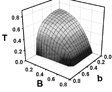
Figure 1: The surface $|W|=1$ in the space of magnetic field, $B$, temperature, $T$, and alternating magnetic field, $b$. The region between the surface and the axes is entangled.

Diagonalization of Hamiltonian - In order to find the partition function of the system, we must diagonalize the Hamiltonian, Eq. (1) and find its energy eigenvalues. The open ended Hamiltonian can be exactly diagonalized in a standard way via several steps: a Jordan-Wigner tansformation, a Fourier transformation and finally a Bogoliubov transformation. The Jordan-Wigner transformation,

$$a_{l}=\prod_{m=1}^{l-1}\sigma_{m}^{z}\otimes\frac{\left(\sigma_{l}^{x}+i\sigma_{l}^{y}\right)}{2},$$ (3)

maps the Pauli spin operators into fermionic annihilation and creation operators $a_{l}$ and $a_{l}^{\dagger}$. These satisfy the anti-commutation relations $\{a_{l},a_{k}\}=0$ and $\{a_{l},a_{k}^{\dagger}\}=\delta_{l,k}$. Preserving the anti-commutation relations, the operators can now be transformed unitarily using a Fourier transformation, $a_{l}=\sqrt{\frac{2}{N+1}}\sum_{k=1}^{N}d_{k}\sin(\frac{\pi kl}{N+1})$ and by a Bogoliubov transformation,

$$d_{k} = \alpha_{k}\cos\theta_{k}+\beta_{k}\sin\theta_{k}$$ (4)

$$d_{N+1-k} = \beta_{k}\cos\theta_{k}-\alpha_{k}\sin\theta_{k}.$$

Setting $\tan 2\theta_{k}=b/[J\cos(\pi k/(N+1))]$ eliminates the off-diagonal terms leaving the Hamiltonian in diagonal form

$$H=\sum_{k=1}^{N/2}\left(\lambda_{k}^{+}\alpha_{k}^{\dagger}\alpha_{k}+\lambda_{k}^{-}\beta_{k}^{\dagger}\beta_{k}-2B{\bf 1}\right)$$ (5)

where $\lambda_{k}^{\pm}=2B\pm 2\sqrt{J^{2}\cos^{2}(\pi k/(N+1))+b^{2}}$. The operators $\alpha_{k}$ and $\beta_{k}$ satisfy the anti-commutation relations $\{\alpha_{k},\alpha_{l}^{\dagger}\}=\{\beta_{k},\beta_{l}^{\dagger}\}=\delta_{k,l}$ and $\{\alpha_{k},\beta_{l}\}=\{\alpha_{k},\beta_{l}^{\dagger}\}=0$. Using the eigenvalues of the Hamiltonian, we find that the partition function can be written $Z=\prod_{k=1}^{N/2}2\cosh\left(\beta\lambda_{k}^{+}/2\right)2\cosh\left(\beta\lambda_{k}^{-}/2\right)$. In the thermodynamic limit, $N\rightarrow\infty$, we can treat $\omega=\pi k/N$ as a continuous variable, to find

$$\ln Z=\frac{N}{\pi}\int_{0}^{\pi/2}d\omega\ln\left[4\cosh\left(\frac{\beta\lambda^{+}_{\omega}}{2}\right)\cosh\left(\frac{\beta\lambda^{-}_{\omega}}{2}\right)\right]$$ (6)

where $\lambda_{\omega}^{\pm}=2B\pm 2\sqrt{J^{2}\cos^{2}\omega+b^{2}}$. We can now use Eq. (2) to calculate the entanglement witness for our system.

The region of entanglement detected by our witness has been plotted in Fig. (1). The figure shows the region of uniform magnetic field, $B$, temperature, $T$, and alternating magnetic field, $b$, within which we always find entanglement. At fixed values of $b$, the entangled region of the $T-B$ plane shrinks as $b$ increases until a critical value is reached above which entanglement is no longer detected. Consider now a plane perpendicular to the $T$ axis. At zero temperature we see that until the critical value $b_{c}=0.56$, increasing $b$ has no effect on the value that the uniform magnetic field can take with the system remaining in an entangled state. Above $b_{c}$, our witness detects no entanglement. However, we later show that this witness is not optimal at zero temperature.

Our witness shows entanglement behaving as we would expect physically. A high temperature causes the system to become mixed. Thus no quantum correlations can survive and the system is separable. Moreover, the effect of the magnetic fields is understandable as local operations which enhance classical correlations. When the uniform magnetic field becomes large, spins tend to line up in a direction parallel to that field. This clearly decreases quantum correlations in the system. Using the same reasoning, if the alternating magnetic field is large, the spins tend to anti-align which is also a product state. Hence, as Fig. (1) shows, all of these parameters cause the system to become separable if they are large enough. Interestingly, we find a counter example of this expected behaviour and identify a region where the system is entangled even in a large magnetic field. We discuss this in the following section.

Single-site entropy - When $T=0$, the total system is in a pure state, i.e. the ground state. Thus, if the density matrix of a single spin is in a mixed state, the particle must be entangled with the rest of the spins. This can be quantified using the entropy of a single spin. The $l$-th spin density matrix, $\rho_{l}=\frac{1}{2}\sum_{i\in\{1,x,y,z\}}\sigma_{l}^{i}\langle\sigma_{l}^{i}\rangle$, can be obtained from the total density matrix $\rho=e^{-\beta\hat{H}}/Z$. Moreover, we find that the single-site density matrix is readily diagonalized since $\langle\sigma_{l}^{x}\rangle=\langle\sigma_{l}^{y}\rangle=0$. This follows from the fact that $\sigma_{l}^{x}$ and $\sigma_{l}^{y}$ are linear combinations of the fermion operators $\alpha_{k}$, $\alpha_{k}^{\dagger}$, $\beta_{k}$, and $\beta_{k}^{\dagger}$, all of which have zero expectation values.

In the thermodynamic limit $N\to\infty$, the system is translationally invariant for all odd sites and for all even sites. Hence the single-site magnetization $\langle\sigma_{l}^{z}\rangle$ can be obtained from the total magnetization $M$ and the total staggered magnetization $M_{\mathrm{s}}$. In the limit of zero temperature, these are given by

$$M = \sum_{l}\langle\sigma_{l}^{z}\rangle=\frac{1}{\beta}\frac{\partial}{\partial B}\ln Z=N\left(1-\frac{2\Omega}{\pi}\right)$$ (7)

$$M_{\mathrm{s}} = \sum_{l}(-1)^{l}\langle\sigma_{l}^{z}\rangle=\frac{1}{\beta}\frac{\partial}{\partial b}\ln Z=\frac{N}{\pi}\int_{0}^{\Omega}d\omega f(\omega)$$

where $f(\omega)=2b/\sqrt{J^{2}\cos^{2}\omega+b^{2}}$ and

$$\Omega=\left\{\begin{array}[]{lcl}\pi/2&\mbox{for}&B<b\\ \cos^{-1}\Big{(}\sqrt{B^{2}-b^{2}}/J\Big{)}&\mbox{for}&b\leq B\leq\sqrt{J^{2}+b^{2}}\\ 0&\mbox{for}&B>\sqrt{J^{2}+b^{2}}\end{array}\right.$$

To obtain these results, we have used $\lim_{\beta\rightarrow\infty}\tanh(\beta x)=x/|x|$. By virtue of translational invariance, $\langle\sigma_{l}^{z}\rangle$, is the same for all even sites and for all odd sites. Thus defining $\langle\sigma^{z}_{l}\rangle=\mbox{Tr}(\sigma^{z}_{l}\rho)=2\eta_{l}-1$, such that the single-site density matrix is $\rho_{l}=\mbox{diag}(\eta_{l},1-\eta_{l})$, we have

$$\eta_{l}=\frac{1}{2}\Big{\{}1+\frac{1}{N}\left[M+(-1)^{l}M_{\mathrm{s}}\right]\Big{\}}.$$ (8)

From this, we can obtain the entropy of the $l$-th spin, $S=-\eta_{l}\log_{2}\eta_{l}-(1-\eta_{l})\log_{2}(1-\eta_{l})$.

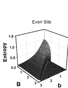
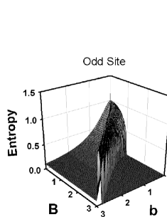
Figure 2: We plot the entropy for an even site spin and an odd site spin respectively when $T=0$ and $J=1$. Excluding the region $B>\sqrt{1+b^{2}}$, the single-site entropy is non zero and each spin is entangled with the rest of the system. The odd site entropy shows a maximum when $B=b+\varepsilon$.

The single-site entropy for odd and even sites is plotted in Fig. (2) with $J=1$. In both cases, we find entanglement for various values of $B$ and $b$ even when the magnetic fields are large. The entropy, and therefore entanglement between each spin and the remainder of chain, is non-zero everywhere except when $B>\sqrt{J^{2}+b^{2}}$. Hence entanglement exists when the coupling strength between nearest neighbour spins, $J$, is more than $\sqrt{B^{2}-b^{2}}$. We note that this corresponds to when the square of the interaction strength is greater than the product of the total magnetic field on two adjacent sites. In addition, we observe from Fig. (2) that the maximum single-site entropy occurs when both magnetic fields $B$ and $b$ are zero. Introducing the magnetic fields reduces the amount of entanglement in the system except along the peak in the odd site entropy. We find from the maximum entropy, $S_{l}=1$, that the maximum entanglement occurs in the region $b\leq B\leq\sqrt{J^{2}+b^{2}}$ when $\Omega-\pi/2=(-1)^{l}\int_{0}^{\Omega}b/\sqrt{J^{2}\cos^{2}\omega+b^{2}}d\omega$ is satisfied. This corresponds to when the magnetization, $M$, is equal to the staggered magnetization, $M_{\mathrm{s}}$. For even sites, there is only one solution to this at $B=b=0$. For odd sites however, this is satisfied for any finite uniform magnetic field $B$ at $B=b+\varepsilon$ where $\varepsilon$ is a positive value. The solutions in Fig. (3) correspond to the peak in the odd site entropy and so occur within the range $b\leq B\leq\sqrt{J^{2}+b^{2}}$. In general, $\varepsilon$ becomes larger as $J$ increases as shown in Fig. (3), and becomes smaller as $B$ and $b$ increase. We note that the peak does not occur at $B=b$. As $B$ and/or $b$ tend to infinity, the amount of entanglement in the system tends to zero. Further, as the magnetic fields increase, the curves in Fig. (3) tend to the $B=b$ line. At $B=b$, the system is no longer maximally entangled. At this point, we find from the Hamiltonian that odd sites have zero magnetic field, and even sites have field strength $2B$. Hence at the peak, odd site spins have a small magnetic field, $\varepsilon$, while in comparison, even site spins have a large field, $2B-\varepsilon$. The implications of this peak are that even in the limit of large (though not infinite) uniform field $B$, an odd site can be maximally entangled with the rest of the system if an appropriate alternating magnetic field, $b$ is introduced. In practice, fine-tuning $b$ to achieve maximal entanglement may be difficult. However, for any $B$, sufficiently increasing $b$ (when $b>\sqrt{B^{2}-J^{2}}$) will create entanglement in the chain. Hence a staggered magnetic field can enhance the amount of entanglement present in the system.

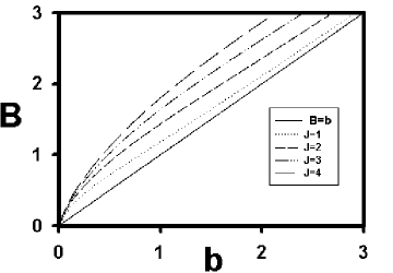
Figure 3: Plot of the maximum entropy $S_{l}=1$ for odd site spins with different values of $J$. As the value of $J$ increases, this maximum entropy moves further away from the line $B=b$.

Although the single-site entanglement relates only to the zero temperature case, changing the temperature by a small amount should not change its behaviour. Hence for very low temperatures, we see that the entanglement witness is not optimal.

Conclusions - Our best estimate for finite temperature entanglement is the witness which shows $b$ reduces the region of entanglement in the chain. That is, a staggered magnetic field reduces the entangled region. If this behaviour is true even for an optimal finite temperature witness, these results have consequences for larger scale quantum computation in solid state systems. As inhomogeneities in the magnetic field exist naturally in the Zeeman coupling between atoms, the region of entanglement is naturally decreased compared to when $b=0$. Quantum computation relies on entanglement so as introducing $b$ reduces both the temperature and uniform magnetic field at which entanglement persists, our result shows it may be more difficult than previously thought to construct useful quantum computers using one-dimensional systems.

Our entanglement witness is invaluable as by applying it to our system, it allows us to see how temperature affects the entanglement in the spin chain. However, the witness does not tell us how the entanglement actually behaves in the presence of $B$, $T$ or $b$ as it does not detect all entanglement in the system. Conversely, the single-site entropy shows us exactly how the entanglement is affected by the magnetic fields at zero temperature, although it is unknown how to extend this entropy to a finite temperature. Using this entropy, we have shown that in the thermodynamic limit, a staggered magnetic field enhances both the region and the amount of entanglement in our spin chain. Hence, both the witness and the entropy are essential in characterizing the entanglement in the system. Further, the region of entanglement identified by the witness is consistent with that of the single-site entropy. If the behaviour of the entanglement as shown by the entropy persists at higher temperatures, we may be able to counteract any Zeeman coupling by applying an appropriate magnetic field, hence maximizing entanglement for odd sites. This will be an interesting topic for future research.

Acknowledgement - V.V. & J.H. acknowledge the EPSRC for financial support.

References

- (1) A. Einstein, B. Podolsky and N. Rosen, Phys. Rev. 47, 777 (1935)
- (2) D. Loss, D.P. DiVincenzo, Phys. Rev. A 57, 120 (1998)
- (3) A. Imamoglu, D.D. Awschalom, G. Burkard, D.P. DiVincenzo, D. Loss, M. Sherwin, and A. Small, Phys. Rev. Lett. 83, 4204 (1999)
- (4) D.P. Divincenzo et al. Nature, 408, 339 (2000)
- (5) X. Wang, Phys. Rev. A, 64, 012313 (2001)
- (6) M. C. Arnesen, S. Bose, V. Vedral, Phys. Rev. Lett. 87, 017901 (2001)
- (7) C. Brukner, V. Vedral, quant-ph/0406040 (2004)
- (8) M. R. Dowling, A. C. Doherty, S. D. Bartlett, Phys. Rev. A 70, 062113 (2004)
- (9) G. Toth, Phys. Rev. A, 71, 010301(R) (2005)
- (10) L. A. Wu, S. Bandyopadhyay, M. S. Sarandy, D. A. Lidar, Phys. Rev. A 72, 032309 (2005)
- (11) M. Oshikawa, I. Affleck, Phys. Rev Lett. 79, 2883 (1997)
- (12) H. Nojiri, Y. Ajiro, T. Asano, J. P. Boucher, New J. Phys. 8, 218 (2006)
- (13) M. Wiesniak, V. Vedral, C. Brukner, New J. Phys. 7, 258 (2005)
- (14) S. Ghosh, T. F. Rosenbaum, G. Aeppli, S. N. Coppersmith, Nature 425, 48 (2003)
- (15) V. Vedral, Nature 425, 28 (2003)
- (16) M. Suzuki, J. Phys. Soc. Japan, 21, 2140 (1966)
- (17) S. Katsura, Phys. Rev. 127, 1508 (1962)
- (18) S. Katsura, Phys. Rev. 129, 2835 (1963)
- (19) M. Horodecki, P. Horodecki, R. Horodecki, Phys. Lett. A, 223, 1 (1996)