Theory of Dicke narrowing in coherent population trapping

O. Firstenberg Department of Physics, Technion-Israel Institute of Technology, Haifa 32000, Israel    M. Shuker Department of Physics, Technion-Israel Institute of Technology, Haifa 32000, Israel    A. Ben-Kish Department of Physics, Technion-Israel Institute of Technology, Haifa 32000, Israel    D. R. Fredkin Department of Physics, University of California, San Diego, La Jolla, California 92093    N. Davidson Department of Physics of Complex Systems, Weizmann Institute of Science, Rehovot 76100, Israel    A. Ron Department of Physics, Technion-Israel Institute of Technology, Haifa 32000, Israel
Abstract

The Doppler effect is one of the dominant broadening mechanisms in thermal vapor spectroscopy. For two-photon transitions one would naively expect the Doppler effect to cause a residual broadening, proportional to the wave-vector difference. In coherent population trapping (CPT), which is a two-photon narrow-band phenomenon, such broadening was not observed experimentally. This has been commonly attributed to frequent velocity-changing collisions, known to narrow Doppler-broadened one-photon absorption lines (Dicke narrowing). Here we show theoretically that such a narrowing mechanism indeed exists for CPT resonances. The narrowing factor is the ratio between the atom’s mean free path and the wavelength associated with the wave-vector difference of the two radiation fields. A possible experiment to verify the theory is suggested.

pacs:
42.50.Gy, 32.70.Jz
preprint:

I Introduction

The spectral line shape of atomic transitions is determined by many different mechanisms Wittke and Dicke (1956). Specifically, a Doppler-broadened spectrum can be dramatically narrowed due to frequent velocity-changing collisions — Dicke narrowing Dicke (1953); Galatry (1961). The narrowing factor is proportional to the ratio between the collisions mean free path and the radiation wavelength. Dicke narrowing was observed for microwave transitions Budker et al. (2005) and recently also for optical transitions Dutier et al. (2003). For two-photon transitions, such as coherent population trapping (CPT) Arimondo (1996), a dramatic narrowing of the expected Doppler-width was also observed and was attributed to a Dicke-like narrowing Cyr et al. (1993); Nagel et al. (1999); Vanier et al. (2003); Dutier et al. (2005). CPT is a light-matter interaction involving three-level atoms and two 
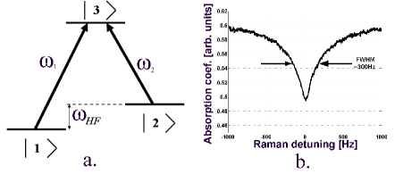
resonant radiation fields (see figure 1.a). The atoms are driven into a coherent superposition of the lower levels, |1ket1\left|1\right\rangle and |2ket2\left|2\right\rangle which does not absorb the radiation. The efficiency of this process strongly depends on the Raman (two-photon) detuning, defined as ΔR=ωHF(ω1ω2)subscriptΔ𝑅subscript𝜔HFsubscript𝜔1subscript𝜔2\Delta_{R}=\omega_{\text{HF}}-(\omega_{1}-\omega_{2}). Therefore, when scanning the frequency of one of the lasers, an absorption dip is observed, which we will refer to as a CPT resonance (see figure 1.b).

Refer to caption
Figure 1: a. Energy levels scheme of CPT system. Two laser fields with frequencies $\omega_{1},\omega_{2}$ excite two levels to a common upper level. b. Typical measurement of a CPT resonance in room temperature 87Rb vapor, with frequency difference of $\omega_{\text{HF}}=6.834$GHz. The residual Doppler broadening is about $10$KHz, while the measured width is only about $300$Hz.

The narrow width of CPT resonances is useful for several applications such as frequency standards Cyr et al. (1993); Knappe et al. (2004), magnetometers Schwindt et al. (2004), slow and stored light Lukin (2003); Fleischhauer et al. (2005). In all the applications a key parameter is the spectral width of the CPT resonance. When the CPT is performed in room-temperature vapor, the two radiation fields experience a Doppler shift which is different for each atomic velocity group. In the case of non-degenerate lower levels (e.g. two hyperfine levels in the ground state of an alkali atom) or for non-collinear laser beams, the two radiation fields experience slightly different Doppler shifts. This difference, denoted as the residual Doppler shift, results in an effective Raman detuning which is different for each velocity group. Therefore, one would naively expect a residual Doppler broadening of the CPT resonance. However, the measured CPT resonance width is well below the expected residual Doppler width. For example, the clock-transition CPT resonance of room temperature Rubidium vapor is expected to have a residual Doppler width of

$$\Gamma_{D}^{\text{res}}=\frac{v_{\text{th}}}{c}\omega_{\text{HF}}\approx 10\text{KHz,}$$ (1)

where $v_{\text{th}}$ is the thermal velocity, $\omega_{\text{HF}}$ is the hyperfine energy-gap, and $c$ is the speed of light. However, a typical measurement of this CPT resonance, depicted in figure 1.b, shows a width of only $300$Hz. In order to attribute this dramatic narrowing to a Dicke-like narrowing effect, one commonly assumes that the wavelength which determines the narrowing factor is the one associated with the frequency difference of the lasers (i.e. the microwave frequency) Cyr et al. (1993). In Ref. Erhard and Helm (2001) a numerical model was used to calculate the CPT line-shape, introducing discrete velocity groups, and indeed demonstrated the expected narrowing. In the present work we derive an analytic expression for the line-shape of CPT resonances, that demonstrates both Doppler broadening and collisions-induced Dicke narrowing. We show that in a regime relevant to most CPT experiments, the narrowing is governed by the ratio between the mean free path and the wavelength associated with the wave-vector difference of the lasers. In section II we review the two-level Dicke narrowing. In section III we derive the theory for Dicke narrowing of CPT resonances. Section IV contains a discussion of the results and presents a possible experimental setup to verify this result.

II Dicke narrowing of two-level atoms absorption line

In this section, as an introduction to the CPT case, we develop a theory for the line-shape of a two-level atom, including both Doppler broadening and Dicke narrowing. Our approach is similar to that presented by Galatry Galatry (1961). We consider a two-level atom with the upper and lower states, $\left|3\right\rangle$ and $\left|1\right\rangle$, and an optical energy gap of $\hbar\omega_{0}$. We assume that the kinetic energy of the atom is much smaller than $\hbar\omega_{0}$ and take the motion of the center of mass of the atom to be classical. The atom interacts with an external, classical electromagnetic field, with wave-vector $\mathbf{q}$ and frequency $\omega=c\left|\mathbf{q}\right|$. We assume that $\omega$ is of the order of $\omega_{0}$ and express the Hamiltonian in the dipole approximation and the rotating wave approximation as

$$H=\hbar\omega_{0}\left|3\right\rangle\left\langle 3\right|-\left[\hbar\Omega e^{i\left(\mathbf{q\cdot r}-\omega t\right)}\left|3\right\rangle\left\langle 1\right|+\text{H.c.}\right]\text{,}$$ (2)

where $\Omega$ is the Rabi frequency of the field and $\mathbf{r}=\mathbf{r}\left(t\right)$ is the time-dependent center of mass position of the atom. The equations of motion of the density matrix elements $\rho\,_{3,3}$ and $\rho_{3,1}$ are given by:

$\displaystyle\dot{\rho}_{3,1}$ $\displaystyle=-i\left(\omega_{0}-i\Gamma\right)\rho_{3,1}-i\Omega e^{i\left(\mathbf{q\cdot r}-\omega t\right)}\left(2\rho_{3,3}-1\right)$ (3a)
$\displaystyle\dot{\rho}_{3,3}$ $\displaystyle=-2\Gamma\rho_{3,3}+2\operatorname{Im}\Omega^{\ast}e^{-i\left(\mathbf{q\cdot r}-\omega t\right)}\rho_{3,1}.$ (3b)
Here we assumed a single relaxation term (radiation bath), which induces transitions between the atomic levels $\left(\left|3\right\rangle\rightarrow\left|1\right\rangle\right),$ with the rate $\Gamma$ Cohen-Tannoudji et al. (1992). In order to calculate the absorption spectrum, we write the energy absorption $\dot{W}\left(t\right),$ in terms of the population response to the applied field:
$$\dot{W}\left(t\right)=\hbar\omega_{0}\left\{\dot{\rho}_{3,3}\right\}_{\text{field}}=2\hbar\omega_{0}\operatorname{Im}\left(\Omega^{\ast}e^{-i\left(\mathbf{q\cdot r}-\omega t\right)}\rho_{3,1}\right).$$ (4)

In the steady-state we take the temporal average, and find the absorption spectrum $S\left(\omega\right)$ to be:

$$S\left(\omega\right)=\frac{\overline{\dot{W}\left(t\right)}}{2\hbar\omega_{0}\left|\Omega\right|^{2}}=\operatorname{Im}\lim_{T\rightarrow\infty}\int_{0}^{T}\frac{dt}{T}\frac{\rho_{3,1}\left(t\right)}{\Omega e^{i\left(\mathbf{q\cdot r}-\omega t\right)}}.$$ (5)

We consider the unsaturated case in which $\Omega\ll\Gamma$, and use the perturbation expansion of $\dot{\rho}\left(t\right)$. Taking the initial state of the atom to be the ground state, we find to zero order in $\Omega$ that $\rho_{3,3}^{(0)}\left(t\right)=\rho_{3,1}^{(0)}\left(t\right)=0$, and to the first order that

$$\dot{\rho}_{3,1}^{\left(1\right)}=-i\left(\omega_{0}-i\Gamma\right)\rho_{3,1}^{\left(1\right)}-i\Omega e^{i\left(\mathbf{q\cdot r}-\omega t\right)}\left(2\rho_{3,3}^{(0)}-1\right),$$ (6)

with the formal solution

$$\rho_{3,1}^{\left(1\right)}\left(t\right)=i\Omega\int_{0}^{t}dt^{\prime}e^{-i\left(\omega_{0}-i\Gamma\right)\left(t-t^{\prime}\right)}e^{i\mathbf{q\cdot r}\left(t^{\prime}\right)-i\omega t^{\prime}}.$$ (7a)
Substituting $\rho_{3,1}^{\left(1\right)}\left(t\right)$ in Eq.(5), denoting $\tau=t-t^{\prime}$ and taking the upper limit of the $\tau-$integral to infinity, we obtain in steady-state,
$$S\left(\omega\right)=\operatorname{Re}\int_{0}^{\infty}d\tau e^{-i\left(\Delta-i\Gamma\right)\tau}\overline{e^{i\Phi\left(\tau\right)}},$$ (8)

where $\Delta=\omega-\omega_{0}$ is the detuning from resonance,

$$\Phi\left(\tau\right)=\mathbf{q\cdot}\left[\mathbf{r}\left(\tau\right)-\mathbf{r}\left(0\right)\right],$$ (9)

is the phase accumulated during $\tau$ and the average is over atom trajectories,

$$\overline{e^{i\Phi\left(\tau\right)}}=\lim_{T\rightarrow\infty}\frac{1}{T}\int_{0}^{T}dte^{i\mathbf{q\cdot}\left[\mathbf{r}\left(t\right)-\mathbf{r}\left(t-\tau\right)\right]}.$$ (10)

Notice that the accumulated phase includes both the Doppler effect and collisions. Assuming that $\Phi\left(\tau\right)$ is a random Gaussian variable and following the cumulant expansion procedure Abramowitz and Stegun (1972), we substitute $\overline{e^{i\Phi\left(\tau\right)}}=e^{-\overline{\Phi\left(\tau\right)^{2}}/2}.$ Following Eq.(9) we write

$$\Phi\left(\tau\right)=\sum_{\alpha}q^{\alpha}\int_{o}^{\tau}dt_{1}u^{\alpha}\left(t_{1}\right),$$ (11)

where $u^{\alpha}$ are the velocity cartesian components and $\alpha=x,y,z$, to get

$\displaystyle\overline{\Phi\left(\tau\right)^{2}}$ $\displaystyle=\sum_{\alpha,\alpha^{\prime}}q^{\alpha}q^{\alpha^{\prime}}\int_{0}^{\tau}dt_{1}\int_{0}^{\tau}dt_{2}\overline{u^{\alpha}\left(t_{1}\right)u^{\alpha^{\prime}}\left(t_{2}\right)}$
$\displaystyle=2\sum_{\alpha,\alpha^{\prime}}q^{\alpha}q^{\alpha^{\prime}}\int_{0}^{\tau}dt\left(\tau-t\right)\overline{u^{\alpha}\left(t\right)u^{\alpha^{\prime}}\left(0\right)}.$ (12)

As shown in the appendix, the velocity-velocity correlation function is given approximately by

$$\overline{u^{\alpha}\left(t\right)u^{\alpha^{\prime}}\left(0\right)}=\delta_{\alpha^{\prime}\alpha}v_{\text{th}}^{2}e^{-\gamma\left|t\right|},$$ (13)

where $\delta_{\alpha,\alpha^{\prime}}$ is the Kronecker Delta, $v_{\text{th}}$ is the thermal velocity and $\gamma$ is interpreted as the velocity relaxation rate (for the Brownian motion regime) or as the collisions rate (for the strong collisions regime). Substituting this in Eq.(12) gives

$$\overline{\Phi\left(\tau\right)^{2}}=2q^{2}v_{\text{th}}^{2}\int_{0}^{\tau}dt\left(\tau-t\right)e^{-\gamma t}=\frac{2q^{2}v_{\text{th}}^{2}}{\gamma^{2}}G\left(\gamma\tau\right)$$ (14)

where

$$G\left(x\right)=x-1+e^{-x}.$$ (15)

Then the absorption spectrum, Eq.(8), is written as

$$S\left(\omega\right)=\int_{0}^{\infty}d\tau e^{-\Gamma\tau-\Gamma_{D}^{2}G\left(\gamma\tau\right)/\gamma^{2}}\cos\left(\Delta\tau\right),$$ (16)

where $\Gamma_{D}=qv_{\text{th}}=\omega v_{\text{th}}/c$ is the Doppler width. Restricting the discussion to the regime where $\Gamma_{D}\gg\Gamma,$ one finds two limits Galatry (1961):

(i) The Doppler limit, $\gamma\ll\Gamma_{D}$, where the quadratic term $G\left(\gamma\tau\right)\approx\gamma^{2}\tau^{2}/2$ is dominant and the absorption spectrum,

$$S_{\text{Doppler}}\left(\omega\right)=\sqrt{\frac{\pi}{2}}\frac{1}{\Gamma_{D}}e^{-\frac{\Delta^{2}}{2\Gamma_{D}^{2}}},$$ (17)

is the well-known Doppler-broadened spectrum. The same expression is usually derived by a convolution of the homogenous line shape with the thermal velocity distribution.

(ii) The Dicke limit, $\gamma\gg\Gamma_{D}$, where the linear term $G\left(\gamma\tau\right)\approx\gamma\tau$ is dominant and the absorption spectrum,

$$S_{\text{Dicke}}\left(\omega\right)=\frac{\Gamma+\Gamma_{D}^{2}/\gamma}{\Delta^{2}+\left(\Gamma+\Gamma_{D}^{2}/\gamma\right)^{2}},$$ (18)

is a Lorentzian with natural-width ΓΓ\Gamma, broadened by ΓD2/γ.superscriptsubscriptΓ𝐷2𝛾\Gamma_{D}^{2}/\gamma. Denoting the mean free path Λ=vth/γ,Λsubscript𝑣th𝛾\Lambda=v_{\text{th}}/\gamma, and the field’s wavelength λ=2π/q𝜆2𝜋𝑞\lambda=2\pi/q, we find the line-width to be Γ+(2πΛ/λ)ΓD,Γ2𝜋Λ𝜆subscriptΓ𝐷\Gamma+\left(2\pi\Lambda/\lambda\right)\Gamma_{D}, showing that the Doppler broadening is effectively reduced by a factor known as the Dicke 
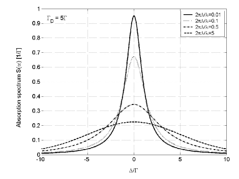
parameter Dicke (1953). A numerical solution of Eq.(16), showing the transition between the Doppler and the Dicke limits, is shown in Fig.(2).

Refer to caption
Figure 2: The effect of Dicke narrowing on the absorption spectrum: a numerical solution of Eq.(16) for several values of the Dicke parameter $2\pi\Lambda/\lambda$, with $\Gamma_{D}=5\Gamma.$

III Dicke narrowing of CPT resonances

We now turn to analyze the line-shape of CPT resonances in the presence of thermal motion and velocity-changing collisions. Consider a three-level atom in a $\Lambda-$configuration, with the energy levels $E_{3}>E_{2}>E_{1}$ corresponding to an upper state $\left|3\right\rangle$ and two lower states $\left|2\right\rangle,\left|1\right\rangle$ (see figure 1.a). We will denote the atomic frequencies $\omega_{nn^{\prime}}=\left(E_{n}-E_{n^{\prime}}\right)/\hbar.$ The atom interacts with external probe and pump electric fields, close to resonance with the $\left|3\right\rangle\rightarrow\left|1\right\rangle$ and $\left|3\right\rangle\rightarrow\left|2\right\rangle$ transitions, respectively. The coupling Hamiltonian is

$$H_{C}=-\hbar\sum_{n=1,2}\Omega_{n}e^{i\mathbf{q}_{n}\mathbf{\cdot r}\left(t\right)-i\omega_{n}t}\left|3\right\rangle\left\langle n\right|+\text{H.c.}$$ (19)

where $\mathbf{q}_{n}$ are the wave-vectors of the fields and $\omega_{n}=c\left|\mathbf{q}_{n}\right|$. For brevity, we denote

$$\Omega_{n}\left(t\right)=\Omega_{n}e^{i\mathbf{q}_{n}\mathbf{\cdot r}\left(t\right)-i\omega_{n}t}~{}~{}~{}~{}n=1,2.$$ (20)

We consider both dipole relaxation terms, which induce transitions between the excited and ground levels$~{}\left|3\right\rangle\rightarrow\left|n\right\rangle$ with rates $\Gamma_{n}$ ($n=1,2$), and within the ground state $\left|1\right\rangle\leftrightarrow\left|2\right\rangle$ with rate $\Gamma_{2\leftrightarrow 1}$; and a spin-boson relaxation term, which induces adiabatic transitions (decoherence) between $\left|1\right\rangle\leftrightarrow\left|2\right\rangle$ with rate $\Gamma_{ad}$. For an atomic vapor in the presence of a buffer gas, $\Gamma_{n}$ will be the pressure-broadened homogenous width. The equations of motion for the density matrix are thus

$\displaystyle\dot{\rho}_{1,1}$ $\displaystyle=-2\operatorname{Im}\Omega_{1}^{\ast}\left(t\right)\rho_{3,1}+\Gamma_{1}\rho_{3,3}+\Gamma_{2\leftrightarrow 1}\left(\rho_{2,2}-\rho_{1,1}\right)$
$\displaystyle\dot{\rho}_{2,2}$ $\displaystyle=-2\operatorname{Im}\Omega_{2}^{\ast}\left(t\right)\rho_{3,2}+\Gamma_{2}\rho_{3,3}-\Gamma_{2\leftrightarrow 1}\left(\rho_{2,2}-\rho_{1,1}\right)$
$\displaystyle\dot{\rho}_{3,3}$ $\displaystyle=2\operatorname{Im}\left[\Omega_{1}^{\ast}\left(t\right)\rho_{3,1}+\Omega_{2}^{\ast}\left(t\right)\rho_{3,2}\right]-\left(\Gamma_{1}+\Gamma_{2}\right)\rho_{3,3}$
$\displaystyle\dot{\rho}_{2,1}$ $\displaystyle=i\Omega\,_{2}^{\ast}\left(t\right)\rho_{3,1}-i\Omega\,_{1}\left(t\right)\rho_{2,3}-i\left(\omega_{21}-i\Gamma_{21}\right)\rho_{2,1}$
$\displaystyle\dot{\rho}_{3,1}$ $\displaystyle=-i\Omega_{1}\left(t\right)\left(\rho_{3,3}-\rho_{1,1}\right)+i\Omega_{2}\left(t\right)\rho_{2,1}$
$\displaystyle-i\left(\omega_{31}-i\Gamma_{C}\right)\rho_{3,1}$
$\displaystyle\dot{\rho}_{3,2}$ $\displaystyle=-i\Omega_{2}\left(t\right)\left(\rho_{3,3}-\rho_{2,2}\right)+i\Omega_{1}\left(t\right)\rho_{1,2}$
$\displaystyle-i\left(\omega_{32}-i\Gamma_{C}\right)\rho_{3,2}$ (21)

where $\Gamma_{C}=\left(\Gamma_{1}+\Gamma_{2}+\Gamma_{2\leftrightarrow 1}+\Gamma_{ad}\right)/2$ , $\Gamma_{21}=\Gamma_{2\leftrightarrow 1}+2\Gamma_{ad}$. To find the absorption spectrum of the probe field, we follow Eqs.(4)-(5) using the response terms of the probe and get,

$$S\left(\omega_{1}\right)=\operatorname{Im}\lim_{T\rightarrow\infty}\int_{0}^{T}\frac{dt}{T}\frac{\rho_{3,1}\left(t\right)}{\Omega_{1}\left(t\right)}.$$ (22)

We consider the standard weak probe case, namely $\Omega_{1}\ll\Omega_{2},$ and avoid saturation by assuming $\Omega_{2}$ smaller than any of the relaxation rates $\Gamma_{n\rightarrow n^{\prime}}.$ The perturbation solution of Eqs.(21) can easily be done, following the same procedure as in the two-level case. To zero order in $\Omega_{1},$ with the initial state $\rho\left(0\right)=\left|1\right\rangle\left\langle 1\right|,$ we find $\rho_{1,1}^{(0)}=1$ and all other matrix elements vanish. To the first order in $\Omega_{1}$,

$\displaystyle\dot{\rho}_{3,1}^{(1)}$ $\displaystyle=i\Omega_{2}\left(t\right)\rho_{2,1}^{(1)}+i\Omega_{1}\left(t\right)-i\left(\omega_{31}-i\Gamma_{1}\right)\rho_{3,1}^{(1)}$ (23a)
$\displaystyle\dot{\rho}_{2,1}^{(1)}$ $\displaystyle=i\Omega\,_{2}^{\ast}\left(t\right)\rho_{3,1}^{(1)}-i\left(\omega_{21}-i\Gamma_{21}\right)\rho_{2,1}^{(1)}$ (23b)
and all other matrix elements vanish. We solve formally Eq.(23b), assuming the initial state vanishes,
$$\rho_{2,1}^{(1)}\left(t\right)=i\int_{0}^{t}dt_{1}\Omega_{2}^{\ast}\left(t_{1}\right)e^{\left(-i\omega_{21}-\Gamma_{21}\right)\left(t-t_{1}\right)}\rho_{3,1}^{(1)}\left(t_{1}\right),$$ (24)

and substitute it back into Eq.(23a),

$\displaystyle\dot{\rho}_{3,1}^{(1)}$ $\displaystyle=i\Omega_{1}\left(t\right)-i\left(\omega_{31}-i\Gamma_{1}\right)\rho_{3,1}^{(1)}$ (25)
$\displaystyle-\Omega_{2}\left(t\right)\int_{0}^{t}dt_{1}\Omega_{2}^{\ast}\left(t_{1}\right)e^{\left(-i\omega_{21}-\Gamma_{21}\right)\left(t-t_{1}\right)}\rho_{3,1}^{(1)}\left(t_{1}\right),$

whose formal solution is an integral equation for $\rho_{3,1}^{(1)}\left(t\right),$

$\displaystyle\rho_{3,1}^{(1)}\left(t\right)$ $\displaystyle=\int_{0}^{t}dt_{2}e^{\left(-i\omega_{31}-\Gamma_{1}\right)\left(t-t_{2}\right)}\left[i\Omega_{1}\left(t_{2}\right)-\right.$ (26)
$\displaystyle\left.\Omega_{2}\left(t_{2}\right)\int_{0}^{t_{2}}dt_{1}\Omega_{2}^{\ast}\left(t_{1}\right)e^{\left(-i\omega_{21}-\Gamma_{21}\right)\left(t_{2}-t_{1}\right)}\rho_{3,1}^{(1)}\left(t_{1}\right)\right].$

An approximate solution for Eq.(26) is obtained by iterations up to first order in $\rho_{3,1}$. It can be shown, by comparing the approximate solution to the exact solution for an atom at rest, that the approximation is valid in the low-contrast regime, when $\left|\Omega_{2}\right|^{2}\ll\Gamma_{12}\Gamma$, i.e. in the limit of small relative increase in transparency. Note that the power-broadening in this regime is small compared to $\Gamma_{12}$.

Performing two iterations of Eq.(26) and returning to Eq.(22), we find the spectrum to be the sum of two terms: (i) The one-photon absorption spectrum,

$$S_{1}=\int_{0}^{\infty}d\tau e^{-\Gamma_{1}\tau-\Gamma_{D}^{2}G\left(\gamma\tau\right)/\gamma^{2}}\cos\left(\Delta_{1}\tau\right)$$ (27)

where $\Gamma_{D}=q_{1}v_{\text{th}}$ and $\Delta_{1}=\omega_{31}-\omega_{1}$ is the one-photon detuning of the probe transition. This is essentially the two-level absorption spectrum, Eq.(16), and is equivalent to the small-signal absorption spectrum in the absence of the pump. (ii) The two-photon absorption dip (the CPT line-shape)

$\displaystyle S_{2}$ $\displaystyle=-\left|\Omega_{2}\right|^{2}\operatorname*{Re}\lim_{T\rightarrow\infty}\int_{0}^{T}\frac{dt}{T}\int_{0}^{t}dt_{1}\int_{0}^{t_{1}}dt_{2}\int_{0}^{t_{2}}dt_{3}$
$\displaystyle e^{\left(-i\Delta_{1}-\Gamma_{1}\right)\left(t-t_{1}+t_{2}-t_{3}\right)}e^{\left(i\Delta_{R}-\Gamma_{21}\right)\left(t_{1}-t_{2}\right)}\times$
$\displaystyle e^{i\mathbf{q}_{2}\mathbf{\cdot}\left[\mathbf{r}\left(t_{1}\right)-\mathbf{r}\left(t_{2}\right)\right]-i\mathbf{q}_{1}\mathbf{\cdot}\left[\mathbf{r}\left(t\right)-\mathbf{r}\left(t_{3}\right)\right]}$ (28)

where $\Delta_{R}=\omega_{1}-\omega_{21}-\omega_{2}$ is the Raman detuning. For brevity, we will take $\Delta_{1}=0$ and write the spectrum in terms of $\Delta_{R}$, i.e. assuming the CPT resonance to occur around the center of the one-photon absorption line. The calculation can easily be generalized to $\Delta_{1}\neq 0$.

To calculate the shape of the absorption dip, we write it as

$\displaystyle S_{2}\left(\Delta_{R}\right)$ $\displaystyle=-\left|\Omega_{2}\right|^{2}\operatorname*{Re}\lim_{T\rightarrow\infty}\int_{0}^{T}\frac{dt}{T}\int_{0}^{t}d\tau e^{\left(i\Delta_{R}-\Gamma_{21}\right)\tau}$
$\displaystyle\int_{0}^{t-\tau}d\tau_{1}e^{-\Gamma_{1}\tau_{1}}\int_{0}^{\tau_{1}}d\tau_{3}e^{iK}$ (29)

where

$$K\equiv\Phi_{2}\left(t-\tau_{3},\tau\right)-\Phi_{1}\left(t,\tau_{1}+\tau\right)$$

and $\Phi_{n}\left(t,\tau\right)\equiv\mathbf{q}_{n}\mathbf{\cdot}\left[\mathbf{r}\left(t\right)-\mathbf{r}\left(t-\tau\right)\right].$ Both the integrations over $\tau$ and $\tau_{1}$ contain exponential decay terms, allowing us to take their upper limits to infinity and average the phase-lag term over $t$,

$\displaystyle S_{2}\left(\Delta_{R}\right)$ $\displaystyle=-\left|\Omega_{2}\right|^{2}\operatorname*{Re}\int_{0}^{\infty}d\tau e^{\left(i\Delta_{R}-\Gamma_{21}\right)\tau}$
$\displaystyle\int_{0}^{\infty}d\tau_{1}e^{-\Gamma_{1}\tau_{1}}\int_{0}^{\tau_{1}}d\tau_{3}\overline{e^{iK}}.$ (30)

In a similar manner to the two-level analysis, we use the cumulant expansion to get

$$\overline{e^{iK}}\approx e^{-\overline{K^{2}}/2}.$$ (31)

Then

$$\overline{K^{2}}=\overline{\Phi_{2}^{2}\left(0,\tau\right)}+\overline{\Phi_{1}^{2}\left(0,\tau_{1}+\tau\right)}-2\overline{\Phi_{2}\Phi_{1}}$$ (32)

where the first two terms can be found from Eq.(14) and the third term is

$$\overline{\Phi_{2}\Phi_{1}}=\overline{\Phi_{2}\left(-\tau_{3},\tau\right)\Phi_{1}\left(0,\tau_{1}+\tau\right)}.$$ (33)

Using Eqs.(11),(13) we find

$\displaystyle\overline{\Phi_{2}\Phi_{1}}$ $\displaystyle=\sum_{\alpha,\alpha^{\prime}}q_{1}^{\alpha}q_{2}^{\alpha^{\prime}}\int_{-\tau_{1}-\tau}^{0}dt_{1}\int_{-\tau_{3}-\tau}^{-\tau_{3}}dt_{2}\overline{u^{\alpha}\left(t_{1}\right)u^{\alpha^{\prime}}\left(t_{2}\right)}$
$\displaystyle=\mathbf{q}_{1}\mathbf{\cdot q}_{2}v_{\text{th}}^{2}\int_{-\tau_{1}-\tau}^{0}dt_{1}\int_{-\tau_{3}-\tau}^{-\tau_{3}}dt_{2}e^{-\gamma\left|t_{2}-t_{1}\right|}.$ (34)

Performing the integral and substituting the results back into Eq.(30), we get

$\displaystyle S_{2}\left(\Delta_{R}\right)$ $\displaystyle=-\left|\Omega_{2}\right|^{2}\operatorname*{Re}\int_{0}^{\infty}d\tau e^{\left(i\Delta_{R}-\Gamma_{21}\right)\tau}e^{-\left(\Gamma_{D}^{\text{res}}/\gamma\right)^{2}G\left(\gamma\tau\right)}$
$\displaystyle\int_{0}^{\infty}d\tau_{1}e^{-\Gamma_{1}\tau_{1}}e^{-\left(\Gamma_{D}/\gamma\right)^{2}\left(\gamma\tau_{1}-e^{-\gamma\tau}+e^{-\gamma\tau}e^{-\gamma\tau_{1}}\right)}$
$\displaystyle\int_{0}^{\tau_{1}}d\tau_{3}e^{\mathbf{q}_{1}\mathbf{\cdot q}_{2}v_{\text{th}}^{2}\left(e^{-\gamma\tau}-1\right)\left(e^{-\gamma\tau_{1}}e^{\gamma\tau_{3}}+e^{-\gamma\tau_{3}}-2\right)/\gamma^{2}}$ (35)

where $G(x)$ was defined in Eq.(15) and

$$\Gamma_{D}^{\text{res}}=\left|\mathbf{q}_{1}-\mathbf{q}_{2}\right|v_{\text{th}}$$ (36)

is the residual Doppler width.

Eq.(35) is a general analytic expression for the CPT line-shape. In what follows we limit the discussion to a specific realistic regime, which is relevent to most CPT experiments. In realizations of CPT in vapor medium, the one-photon processes are usually in the far Doppler regime ($\Gamma_{D}\gg\Gamma_{1}~{}$and $\Gamma_{D}\gg\gamma$) and in most applications the vapor cell contains buffer gas, forcing the two-photon processes into the Dicke regime ($\gamma\gg\Gamma_{D}^{\text{res}}\gg\Gamma_{12}$). Since this regime includes both Doppler and Dicke regimes we denote it as the intermediate regime. As described in the previous section, for the Doppler regime we take $e^{-\gamma\tau_{1}}\approx 1-\gamma\tau_{1},$ and thus $e^{-\gamma\tau_{3}}\approx 1-\gamma\tau_{3}$ and for the Dicke regime we take $e^{-\gamma\tau}\ll 1$ and $G\left(\gamma\tau\right)\approx\gamma\tau$. With these approximations, a simple expression for the CPT line-shape is obtained

$$S_{2}\left(\Delta_{R}\right)=\frac{-\left|\Omega_{2}\right|^{2}}{\left[\Gamma_{1}+\mathbf{q}_{1}\mathbf{\cdot}\left(\mathbf{q}_{1}-\mathbf{q}_{2}\right)v_{\text{th}}^{2}/\gamma\right]^{2}}\frac{\Gamma_{12}+\eta\Gamma_{D}^{\text{res}}}{\Delta_{R}^{2}+\left[\Gamma_{12}+\eta\Gamma_{D}^{\text{res}}\right]^{2}},$$ (37)

where the parameter

$$\eta=\frac{\Gamma_{D}^{\text{res}}}{\gamma}=2\pi\frac{\Lambda}{\lambda_{\text{CPT}}}$$ (38)

is proportional to the ratio between the mean free path, $\Lambda,$ and the wavelength associated with the wave-vector difference, $\lambda_{\text{CPT}}=2\pi/\left|\mathbf{q}_{1}-\mathbf{q}_{2}\right|$. Equation (37) is the main result of the present work, showing that the CPT line-shape is the product of two terms, which are both functions of the wave-vector difference. The first term determines the line’s amplitude and the second is a Lorentzian that determines the width. Since $\eta$ multiplies the residual Doppler width, it acts as a narrowing factor and we denote it as the CPT-Dicke parameter. Finally, in a typical setup of a CPT-based frequency standard Knappe et al. (2004), the laser beams are collinear $\left(\mathbf{q}_{1}\parallel\mathbf{q}_{2}\right)$ and the line-shape can be written as

$$S_{2}^{\parallel}\left(\Delta_{R}\right)=\frac{-\left|\Omega_{2}\right|^{2}}{\left(\Gamma_{1}+\eta\Gamma_{D}\right)^{2}}\frac{\Gamma_{12}+\eta\Gamma_{D}^{\text{res}}}{\Delta_{R}^{2}+\left(\Gamma_{12}+\eta\Gamma_{D}^{\text{res}}\right)^{2}}.$$ (39)

IV Discussion and conclusions

CPT is an inherently narrow-band phenomena usually limited by effective broadening mechanisms. Non-degenerate CPT resonances in a hot vapor cell with buffer gas would naively be broadened by a residual Doppler broadening. However, the measured line-width of CPT resonances are far below the expected residual Doppler width. This effect was attributed to the frequent velocity changing collisions with the buffer gas, that are well known to narrow atomic absorption transitions in two-level atoms. It was also demonstrated using a numerical simulation that when frequent collisions occur no Doppler broadening is evident in the CPT line Erhard and Helm (2001). In this work we developed the theory of Dicke narrowing for CPT resonances in three level atoms. The main result is that the residual Doppler width (that would be observable in an apparatus with no collisions) is diminished by the ratio of the mean free path between collisions and the wavelength associated with the wave-vector difference of the two radiation fields. This theory can be readily extended to describe atoms in confined geometries such as thin vapor cells and cold atoms traps.

For hyperfine CPT experiments, performed in vapor cells with Alkali atoms and several Torrs of buffer gas, the typical CPT-Dicke parameter is $\eta\approx 10^{-4}$ (i.e. very strong Dicke narrowing). Hence the residual Doppler broadening, which is of the order of a few KHz, is strongly reduced and is not measurable (compared to other broadening mechanisms). In order to verify the theoretical prediction it is necessary to increase either the CPT-Dicke parameter or the residual Doppler width. An increase of the CPT-Dicke parameter can be achieved by decreasing the effective wavelength or by increasing the mean free path between collisions. However, changing the effective wavelength is limited by the atomic structure of the active atoms and changing the mean free path will result in a significant diffusion-broadening. We propose to increase the residual Doppler width by introducing a small angular deviation, $\theta$, between the pump and probe beams. For CPT performed with two degenerate lower levels ($\left|\mathbf{q}_{1}\right|=\left|\mathbf{q}_{2}\right|$) and small $\theta$, both the residual Doppler width and the CPT-Dicke parameter are proportional to $\theta$. Therefore, the resulting broadening is proportional to $\theta^{2}$ and can be increased to a measurable level.

Acknowledgements.
We thank Nitsan Aizenshtark for reading the manuscript and helpful suggestions. This work was partially supported by DDRND and the fund for encouragement of research in the Technion.

APPENDIX

To obtain the velocity-velocity correlation function of Eq.(12) we review two simple models:

(i) In the Brownian motion case the equation of motion of the $\alpha$ component of the velocity is

$$\frac{d}{dt}u^{\alpha}\left(t\right)\mathbf{=-}\gamma u^{\alpha}\left(t\right)\mathbf{+}a^{\alpha}\left(t\right)\mathbf{,}$$ (40)

where $\gamma u^{\alpha}\left(t\right)$ is the dynamic frictional force on the atom, $\gamma$ is the velocity relaxation rate, and $a^{\alpha}\left(t\right)$ is the random acceleration Chandrasekhar (1943). For the correlation function we thus obtain

$$\frac{d}{dt}\overline{u^{\alpha}\left(t\right)u^{\alpha^{\prime}}\left(0\right)}\mathbf{=-}\gamma\overline{u^{\alpha}\left(t\right)u^{\alpha^{\prime}}\left(0\right)}+\overline{a^{\alpha}\left(t\right)u^{\alpha^{\prime}}\left(0\right)}\mathbf{,}$$ (41)

where the bar indicates ensemble average. Since the acceleration is not correlated with the initial velocity, the last term on the right vanishes, and we have

$$\overline{u^{\alpha}\left(t\right)u^{\alpha^{\prime}}\left(0\right)}=\overline{u^{\alpha}\left(0\right)u^{\alpha^{\prime}}\left(0\right)}e^{-\gamma\left|t\right|}.$$ (42)

In thermal equilibrium with temperature $T,$ the ensemble average is taken over the velocity distribution function

$$F(\mathbf{u})=\left(m/2\pi k_{B}T\right)^{3/2}e^{-mu^{2}/2k_{B}T},$$ (43)

where $m$ is the mass of the atom, and $k_{B}$ is the Boltzmann factor, and we get

$$\overline{u^{\alpha}\left(0\right)u^{\alpha^{\prime}}\left(0\right)}=\delta_{\alpha^{\prime}\alpha}v_{\text{th}}^{2},$$ (44)

where $\delta_{\alpha,\alpha^{\prime}}$ is the Kronecker Delta, and $v_{\text{th}}=\sqrt{k_{B}T/m}$ is the thermal velocity.

(ii) In the Strong Collisions case the atom is colliding with the dilute buffer gas in thermal equilibrium. The conditional probability density, $f(\mathbf{u},t),$ to find the atom with velocity $\mathbf{u}$ at time $t,$ given that at time $t=0$ its velocity is $\mathbf{u}\left(0\right),$ is given by the Boltzmann collision term,

$$\frac{d}{dt}f(\mathbf{u},t)=-\left[\frac{d}{dt}f(\mathbf{u},t)\right]_{coll},$$ (45)

with the initial distribution

$$f(\mathbf{u},0)=\delta\left(\mathbf{u-u}\left(0\right)\right).$$ (46)

The simplest model is the single relaxation rate approximation, where

$$\left[\frac{d}{dt}f(\mathbf{u},t)\right]_{coll}=\gamma\left(f(\mathbf{u},t)-F(\mathbf{u})\right),$$ (47)

$F(\mathbf{u})$ is the equilibrium distribution of Eq.(43), and $\gamma$ is the collision relaxation rate. The solution of Eq.(45), with Eq.(47), is simply

$$f(\mathbf{u},t)=F(\mathbf{u})\left(1-e^{-\gamma\left|t\right|}\right)+e^{-\gamma\left|t\right|}f(\mathbf{u},0),$$ (48)

and, with Eq.(46), the velocity of the atom at time $t,$ is

$$\mathbf{u}\left(t\right)=\int d^{3}u\mathbf{u}f(\mathbf{u},t)=\mathbf{u}\left(0\right)e^{-\gamma\left|t\right|}.$$ (49)

The velocity-velocity correlation function is

$$\overline{u^{\alpha}\left(t\right)u^{\alpha^{\prime}}\left(0\right)}=\overline{u^{\alpha}\left(0\right)u^{\alpha^{\prime}}\left(0\right)}e^{-\gamma\left|t\right|}.$$ (50)

and since

$$f(\mathbf{u},t\rightarrow\infty)=F(\mathbf{u}),$$ (51)

for consistency

$$\overline{u^{\alpha}\left(0\right)u^{\alpha^{\prime}}\left(0\right)}=\int d^{3}uu^{\alpha}u^{\alpha^{\prime}}F(\mathbf{u})=\frac{k_{B}T}{m}.$$ (52)

We end up in both these models with

$$\overline{u^{\alpha}\left(t\right)u^{\alpha^{\prime}}\left(0\right)}=\delta_{\alpha^{\prime}\alpha}v_{\text{th}}^{2}e^{-\gamma\left|t\right|}.$$ (53)

where the interpretation of $\gamma$ is either the velocity relaxation rate or the collision relaxation rate.

References

  • Wittke and Dicke (1956) J. P. Wittke and R. H. Dicke, Phys. Rev. 103, 620 (1956).
  • Dicke (1953) R. H. Dicke, Phys. Rev. 89, 472 (1953).
  • Galatry (1961) L. Galatry, Phys. Rev. 122, 1218 (1961).
  • Budker et al. (2005) D. Budker, L. Hollberg, D. F. Kimball, J. Kitching, S. Pustelny, and V. V. Yashchuk, Physical Review A (Atomic, Molecular, and Optical Physics) 71, 012903 (pages 9) (2005).
  • Dutier et al. (2003) G. Dutier, A. Yarovitski, S. Saltiel1, A. Papoyan, D. S. ans D. Bloch, and M. Ducloy, Europhysics Letters 63, 35 (2003).
  • Arimondo (1996) E. Arimondo, Progress in Optics, vol. 35 (Elsevier, Amsterdam, 1996).
  • Cyr et al. (1993) N. Cyr, M. Tetu, and M. Breton, IEEE Transactions on Instrumentation and Measurement 42, 640 (1993).
  • Nagel et al. (1999) A. Nagel, C. Affolderbach, S. Knappe, and R. Wynands, Phys. Rev. A 61, 012504 (1999).
  • Vanier et al. (2003) J. Vanier, M. W. Levine, D. Janssen, and M. Delaney, Phys. Rev. A 67, 065801 (pages 4) (2003).
  • Dutier et al. (2005) G. Dutier, P. Todorov, I. Hamdi, I. Maurin, S. Saltiel, D. Bloch, and M. Ducloy, Physical Review A (Atomic, Molecular, and Optical Physics) 72, 040501 (pages 4) (2005).
  • Knappe et al. (2004) S. Knappe, V. Shah, P. D. D. Schwindt, L. Hollberg, J. Kitching, L.-A. Liew, and J. Moreland, Applied Physics Letters 85, 1460 (2004).
  • Schwindt et al. (2004) P. D. D. Schwindt, S. Knappe, V. Shah, L. Hollberg, and J. Kitching, Applied Physics Letters 85, 6409 (2004).
  • Lukin (2003) M. D. Lukin, Reviews of Modern Physics 75, 457 (2003).
  • Fleischhauer et al. (2005) M. Fleischhauer, A. Imamoglu, and J. P. Marangos, Reviews of Modern Physics 77, 633 (2005).
  • Erhard and Helm (2001) M. Erhard and H. Helm, Phys. Rev. A 63, 043813 (2001).
  • Cohen-Tannoudji et al. (1992) C. Cohen-Tannoudji, J. Dupont-Roc, and G. Grynberg, Atom-Photon Interactions (Wiley Interscience, New York, 1992).
  • Abramowitz and Stegun (1972) M. Abramowitz and I. A. Stegun, eds., Handbook of Mathematical Functions with Formulas, Graphs, and Mathematical Tables (Dover, New York, 1972).
  • Chandrasekhar (1943) S. Chandrasekhar, Astrophys. J.  97, 255 (1943).