Quantum Phase Transitions and Matrix Product States in Spin Ladders

Abstract

We investigate quantum phase transitions in ladders of spin $1/2$ particles by engineering suitable matrix product states for these ladders. We take into account both discrete and continuous symmetries and provide general classes of such models. We also study the behavior of entanglement between different neighboring sites near the transition point and show that quantum phase transitions in these systems are accompanied by divergences in derivatives of entanglement.

I Introduction

The basic paradigm of many body physics is to use analytical and numerical tools to investigate the low-lying states and in particular the ground state properties of a system governed by a given Hamiltonian. At very low temperatures, when thermal fluctuations are dominated by quantum fluctuations, quantum phase transitions can occur due to the change of character of the ground state Sachdev . What is exactly meant by ”character” has been investigated in numerous works Osterloh , Nielsen , VedralBose , especially in recent years after the discovery of exact measures Wootters of entanglement(purely quantum mechanical correlations). For example, it has been a matter of debate whether a quantum phase transition is always accompanied by a divergence of some property in entanglement of the ground state wave function.
Unfortunately, except for a few exactly solvable examples, the task of finding the exact ground state of a given Hamiltonian is notoriously difficult. As always in dealing with difficult problems, one way round the difficulty is to investigate the inverse problem, that is to start from states with pre-determined properties and investigate quantum phase transitions which occur by smoothly changing some continuous parameters of these states. The suitable formalism for following this path is the matrix product formalism MPSBasic1 , MPSBasic2 , WolfCirac ; MPSrep which in recent years has been followed in constructing various models of interacting spins mpswork1 ; mpswork2 ; mpswork3 ; mpswork4 ; mpswork5 ; mpswork6 . In this paper we want to take one step in this direction and in particular, we want to construct as concrete models, ladders of spin one-half particles and see what happens to the entanglement between various spins when the system undergoes a phase transition. We construct general class of models having a number of discrete and continuous symmetries. These are symmetry under the exchange of legs of the ladder, symmetry under spin flip, and symmetry under parity (left-right reflection of the ladder) in addition to a continuous symmetry, namely rotation of spins around the $z$ axis or all three axes (full rotational symmetry).
In these models we calculate the entanglement of one rung with the rest of the ladder as measured by the von Neumann entropy of the state of the rung and the entanglement of the two spins of a rung with each other as be measured by the concurrence of the same state.
We will see that in all these models quantum phase transitions occur at a critical point of the coupling constant, and this point is where a rung of the ladder becomes completely disentangled from the rest of the ladder and the two spins of the rung become fully entangled with each other. The derivatives of these two types of entanglement are also divergent.
We should stress here that we are using the term phase transition in a wider sense than usual WolfCirac , that is we call any discontinuity in an observable quantity (i.e. a two point correlation function), a phase transition.

The structure of this paper is as follows. In section II, we review the formalism of Matrix Product States (MPS) with emphasis on the symmetry properties of such states. In section III, we specify the MPS construction to ladders of spin $1/2$ particles and set the general ground for construction of concrete models. In this same section we construct multi-parameter families of models which have specific symmetries. In section IV, we study in detail the properties of the constructed states and in particular calculate the exact correlation functions of spins on the rungs. We also investigate the connection between quantum phase transitions and divergence of entanglement properties in these models. Finally we derive in the appendix, the Hamiltonian which governs the interaction of these models for which the state we have constructed is the exact ground state.

II Matrix Product States

First let us review the basics of matrix product states MPSBasic2 ; WolfCirac . Consider a homogeneous ring of $N$ sites, where each site describes a $d-$level state. The Hilbert space of each site is spanned by the basis vectors $|i\rangle,\ \ i=0,\cdots d-1$. A state

$$|\Psi\rangle=\sum_{i_{1},i_{2},\cdots i_{N}}\psi_{i_{1}i_{2}\cdots i_{N}}|i_{1},i_{2},\cdots,i_{N}\rangle$$ (1)

is called a matrix product state if there exists $D$ dimensional complex matrices $A_{i}\in\mathbb{C}^{D\times D},\ \ i=0\cdots d-1$ such that

$$\psi_{i_{1},i_{2},\cdots i_{N}}=\frac{1}{\sqrt{Z}}tr(A_{i_{1}}A_{i_{2}}\cdots A_{i_{N}}),$$ (2)

where $Z$ is a normalization constant given by

$$Z=tr(E^{N})$$ (3)

and

$$E:=\sum_{i=0}^{d-1}A_{i}^{*}\otimes A_{i}.$$ (4)

Here we are restricting ourselves to translationally invariant states, by taking the matrices to be site-independent. For open boundary conditions, any state can be MPS-represented, provided that we allow site-dependent matrices $A^{(k)}_{i}$, where $k$ denotes the position of the site vidal ; MPSrep . The MPS representation (2) is not unique and a transformation such as $A_{i}\rightarrow UA_{i}U^{-1}$ leaves the state invariant. In view of this we can find the conditions on the matrices which impose discrete symmetries on the state. The state $|\Psi\rangle$ is reflection symmetric if there exists a matrix $U$ such that $A_{i}^{T}=UA_{i}U^{-1}$ where $A^{T}$ is the transpose of $A$ and time-reversal invariant if there exist a matrix $V$ such that $A_{i}^{*}=VA_{i}V^{-1}$.
Let $O$ be any local operator acting on a single site. Then we can obtain the one-point function on site $k$ of the chain $\langle\Psi|O(k)|\Psi\rangle$ as follows:

$$\langle\Psi|O(k)|\Psi\rangle=\frac{tr(E^{k-1}E_{O}E^{N-k})}{tr(E^{N})},$$ (5)

where

$$E_{O}:=\sum_{i,j=0}^{d-1}\langle i|O|j\rangle A_{i}^{*}\otimes A_{j}.$$ (6)

In the thermodynamic limit $N\rightarrow\infty$, equation (5) gives

$$\langle\Psi|O|\Psi\rangle=\frac{\langle\lambda_{max}|E_{O}|\lambda_{max}\rangle}{\lambda_{max}},$$ (7)

where we have used the translation invariance of the model and $\lambda_{max}$ is the eigenvalue of $E$ with the largest absolute value and $|\lambda_{max}\rangle$ and $\langle\lambda_{max}|$ are the right and left eigenvectors corresponding to this eigenvalue, normalized such that $\langle\lambda_{max}|\lambda_{max}\rangle=1$. Here we are assuming that the largest eigenvalue of $E$ is non-degenerate.

The n-point functions can be obtained in a similar way. For example, the two-point function $\langle\Psi|O(k)O(l)|\Psi\rangle$ can be obtained as

$$\langle\Psi|O(k)O(l)|\Psi\rangle=\frac{tr(E_{O}(k)E_{O}(l)E^{N})}{tr(E^{N})}$$ (8)

where $E_{O}(k):=E^{k-1}E_{O}E^{-k}$. Note that this is a formal notation which allows us to write the n-point functions in a uniform way, it does not require that $E$ is an invertible matrix. In the thermodynamic limit the two point function turns out to be

$$\langle\Psi|O(1)O(r)|\Psi\rangle=\frac{1}{\lambda_{max}^{r}}{\sum_{i}\lambda_{i}^{r-2}\langle\lambda_{max}|E_{O}|\lambda_{i}\rangle\langle\lambda_{i}|E_{O}|\lambda_{max}\rangle}.$$ (9)

For large distances $r\gg 1$, this formula reduces to

$$\langle\Psi|O(1)O(r)|\Psi\rangle-\langle\Psi|O|\Psi\rangle^{2}=\frac{\lambda_{1}^{r-2}}{\lambda_{max}^{r}}{\langle\lambda_{max}|E_{O}|\lambda_{1}\rangle\langle\lambda_{1}|E_{O}|\lambda_{max}\rangle},$$ (10)

where $\lambda_{1}$ is the second largest eigenvalue of $E$ for which the matrix element $\langle\lambda_{1}|E_{O}|\lambda_{max}\rangle$ is non-vanishing and we have assumed that the eigenvectors of $E$ have been normalized, i.e. $\langle\lambda_{i}|\lambda_{j}\rangle=\delta_{ij}$. Thus the correlation length is given by

$$\xi=\frac{1}{\ln\frac{\lambda_{max}}{\lambda_{1}}}.$$ (11)

Any level crossing in the largest eigenvalue of the matrix $E$ signals a possible quantum phase transition. Also, due to (11), any level crossing in the second largest eigenvalue of $E$ implies the correlation length of the system has undergone a discontinuous change. Here we are using a broader definition of quantum phase transition, that is we call any non-analytical behavior of a macroscopic property, a quantum phase transition WolfCirac . Of course in the models that we construct we observe a more direct change of observable physical properties, namely in one regime we have correlations between spin operators on different sites and in the other we have no such correlation.

II.1 Symmetries

Consider now a local symmetry operator $R$ acting on a site as $R|i\rangle=R_{ji}|j\rangle$ where summation convention is being used. $R$ is a $d$ dimensional unitary representation of the symmetry. A global symmetry operator ${\cal R}:=R^{\otimes N}$ will then change this state to another matrix product state

$$\Psi_{i_{1}i_{2}\cdots i_{N}}\rightarrow\Psi^{\prime}:=tr(A^{\prime}_{i_{1}}A^{\prime}_{i_{2}}\cdots A^{\prime}_{i_{N}}),$$ (12)

where

$$A^{\prime}_{i}:=R_{ij}A_{j}.$$ (13)

A sufficient but not necessary condition for the state $|\Psi\rangle$ to be invariant under this symmetry is that there exist an operator $U(R)$ such that

$$R_{ij}A_{j}=U(R)A_{i}U^{-1}(R).$$ (14)

Thus $R$ and $U(R)$ are two unitary representations of the symmetry, respectively of dimensions $d$ and $D$. In case that $R$ is a continuous symmetry with generators $T_{a}$, equation (14), leads to

$$(T_{a})_{ij}A_{j}=[{\cal T}_{a},A_{i}],$$ (15)

where $T_{a}$ and ${\cal T}_{a}$ are the $d-$ and $D-$dimensional representations of the Lie algebra of the symmetry. Equations (14) and (15) will be our guiding lines in defining states with prescribed symmetries.

II.2 The Hamiltonian

Given a matrix product state, the reduced density matrix of $k$ consecutive sites is given by

$$\rho_{i_{1}\cdots i_{k},j_{1}\cdots j_{k}}=\frac{tr((A_{i_{1}}^{*}\cdots A_{i_{k}}^{*}\otimes A_{j_{1}}\cdots A_{j_{k}})E^{N-k})}{tr(E^{N})}.$$ (16)

The null space of this reduced density matrix includes the solutions of the following system of equations

$$\sum_{j_{1},\cdots,j_{k}=0}^{d-1}c_{j_{1}\cdots j_{k}}A_{j_{1}}\cdots A_{j_{k}}=0.$$ (17)

Given that the matrices $A_{i}$ are of size $D\times D$, there are $D^{2}$ equations with $d^{k}$ unknowns. Since there can be at most $D^{2}$ independent equations, there are at least $d^{k}-D^{2}$ solutions for this system of equations. Thus for the density matrix of $k$ sites to have a null space it is sufficient that the following inequality holds

$$d^{k}\ >\ D^{2}.$$ (18)

Let the null space of the reduced density matrix be spanned by the orthogonal vectors $|e_{\alpha}\rangle,\ \ \ (\alpha=1,\cdots s,\geq d^{k}-D^{2})$. Then we can construct the local hamiltonian acting on $k$ consecutive sites as

$$h:=\sum_{\alpha=1}^{s}\mu_{\alpha}|e_{\alpha}\rangle\langle e_{\alpha}|,$$ (19)

where $\mu_{\alpha}$’s are positive constants. These parameters together with the parameters of the vectors $|e_{i}\rangle$ inherited from those of the original matrices $A_{i}$, determine the total number of coupling constants of the Hamiltonian. If we call the embedding of this local Hamiltonian into the sites $l$ to $l+k$ by $h_{l,l+k}$ then the full Hamiltonian on the chain is written as

$$H=\sum_{l=1}^{N}h_{l,l+k}.$$ (20)

The state $|\Psi\rangle$ is then a ground state of this hamiltonian with vanishing energy. The reason is as follows:

$$\langle\Psi|H|\Psi\rangle=tr(H|\Psi\rangle\langle\Psi|)=\sum_{l=1}^{N}tr(h_{l,l+k}\rho_{l,l+k})=0,$$ (21)

where $\rho_{l,k+l}$ is the reduced density matrix of sites $l$ to $l+k$ and in the last line we have used the fact that $h$ is constructed from the null eigenvectors of $\rho$ for $k$ consecutive sites. Given that $H$ is a positive operator, this proves the assertion.

III Ladders of spin one-half particles

We now specify the above generalities to a ladder of spin $1/2$ particles. The ladder consists of $N$ rungs and obeys periodic boundary conditions. To each rung of the ladder we associate four matrices $A_{00},\ A_{01},\ A_{10}$ and $A_{11}$ respectively pertaining to the local states $|0,0\rangle,\ |0,1\rangle,\ |1,0\rangle$ and $|1,1\rangle$. Here we are using the qubit notation which corresponds to the spin notation as $|0\rangle=|+\rangle$ and $|1\rangle=|-\rangle.$ The first and the second indices refer respectively to the states of sites on the legs 1 and 2 as shown in figure (1). The rungs are numbered from 1 to N with a periodic boundary condition. The operator $\sigma^{(i)}_{ak}$ refers to the Pauli operator $\sigma_{a}$ on leg number $i$ and the rung number $k$. The total spin operator on a rung at site $k$ is denoted by ${\bf S}_{k}:=\frac{1}{2}(\boldsymbol{\sigma}_{k}^{(1)}+\boldsymbol{\sigma}_{k}^{(2)})$.

III.1 MPS operators for observables

Let us label the legs of the ladder by $1$ and $2$ as in figure (1). In each $A_{ij}$ the first and the second indices refer respectively to legs number 1 and 2.

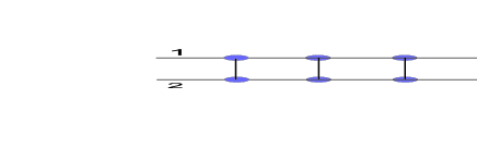
Figure 1: (Color Online) A spin 1/2 ladder, an operator ${\sigma}_{ak}^{(i)}$ refers to the Pauli operator $\sigma_{a}$ on rung $k$ and leg number $(i)$.

Any operator corresponding to leg number $i$ is designated with a superscript $(i)$. With these conventions, one can easily use (6) and write down the MPS operator corresponding to an observable. For example, for the magnetization in the $x$ and $z$ directions in rung 1, we have respectively

$$E_{\sigma_{x}^{(1)}}=A_{00}\otimes A_{10}+A_{10}\otimes A_{00}+A_{01}\otimes A_{11}+A_{11}\otimes A_{01},$$ (22)

and

$$E_{\sigma_{z}^{(1)}}=A_{00}\otimes A_{00}+A_{01}\otimes A_{01}-A_{10}\otimes A_{10}-A_{11}\otimes A_{11}.$$ (23)

For the total magnetization in the $z$ direction in a rung we have

$$E_{S_{z}}=\frac{1}{2}(E_{\sigma_{z}^{(1)}}+E_{\sigma_{z}^{(2)}})=(A_{00}\otimes A_{00}-A_{11}\otimes A_{11}).$$ (24)

Other MPS operators can be obtained in a similar way.

III.2 Symmetries of spin ladders

In this paper we restrict the dimensions of our matrices to $D=2$, and demand that our models have time reversal symmetry so that the matrices $A_{ij}$ are chosen to be real. We will be looking for models which have rotational symmetry in the $x-y$ plane of spin space. Thus we require that there be a matrix ${\cal T}_{z}$ such that

$$[{\cal T}_{z},A_{00}]=A_{00},\ \ \ \ [{\cal T}_{z},A_{11}]=-A_{11},\ \ \ \ [{\cal T}_{z},A_{01}]=[{\cal T}_{z},A_{10}]=0.$$ (25)

It is an easy exercise to show that the solution of these equations is

$$A_{01}=\left(\begin{array}[]{cc}a&0\\ 0&b\end{array}\right),\ \ \ \ A_{10}=\left(\begin{array}[]{cc}a^{\prime}&0\\ 0&b^{\prime}\end{array}\right),\ \ \ \ A_{00}=\left(\begin{array}[]{cc}0&g\\ 0&0\end{array}\right),\ \ \ \ A_{11}=\left(\begin{array}[]{cc}0&0\\ h&0\end{array}\right),$$ (26)

where ${\cal T}$ is found to be ${\cal T}_{z}=\frac{1}{2}\left(\begin{array}[]{cc}1&0\\ 0&-1\end{array}\right)$ and we have excluded the solutions with $g=0$ or $h=0$, which lead to trivial uncorrelated states. Hereafter we use the freedom in re-scaling the matrices (without changing the matrix product state) to set the parameter $h=1$. Let us now consider extra discrete symmetries in addition to the above continuous symmetry. These are as follows:

a: Spin flip symmetry represented by a matrix $X$, such that

$$XA_{i,j}X^{-1}=\epsilon A_{\overline{i},\overline{j}},$$ (27)

where $\epsilon=\pm 1$ and $\overline{i}$ means $i+1\ \ mod\ \ 2$. This symmetry imposes the following condition on the solution (26)

$$a^{\prime}=\epsilon b,\hskip 28.45274ptb^{\prime}=\epsilon a,$$ (28)

where $X$ is found to be $X=\left(\begin{array}[]{cc}0&g\\ \epsilon&0\end{array}\right)$.

b: Symmetry under the exchange of legs of the ladder represented by a matrix $Y$ such that

$$YA_{i,j}Y^{-1}=\eta A_{j,i},$$ (29)

where $\eta=\pm 1$. This symmetry imposes the following condition on (26)

$$a^{\prime}=\eta a,\hskip 28.45274ptb^{\prime}=\eta b,$$ (30)

where $Y$ is found to be $Y=\left(\begin{array}[]{cc}1&0\\ 0&\eta\end{array}\right)$.

c: Parity or a left-right symmetry, represented by a matrix $\Pi$, such that

$$\Pi A_{ij}\Pi^{-1}=\sigma A^{T}_{ij},$$ (31)

with $\sigma=\pm 1$.
This symmetry imposes the condition

$$b=\sigma a,\hskip 28.45274ptb^{\prime}=\sigma a^{\prime},$$ (32)

on (26) where $\Pi$ is found to be $\Pi=\left(\begin{array}[]{cc}0&1\\ \sigma&0\end{array}\right)$.
Thus when we impose any of these discrete symmetries we are left with two three-parameter families of models, each family being distinguished by the discrete parameter $\epsilon$, $\eta$ or $\sigma$.
It is now readily seen that imposing any two of these symmetries makes the model symmetric under the third one too. A model which has all three symmetries is defined by the following set of matrices:

$$A_{01}=\left(\begin{array}[]{cc}a&0\\ 0&\sigma a\end{array}\right),\ \ \ \ A_{10}=\left(\begin{array}[]{cc}\epsilon\sigma a&0\\ 0&\epsilon a\end{array}\right),\ \ \ \ A_{00}=\left(\begin{array}[]{cc}0&g\\ 0&0\end{array}\right),\ \ \ \ A_{11}=\left(\begin{array}[]{cc}0&0\\ 1&0\end{array}\right).$$ (33)

Such matrices satisfy (29) with $\eta=\epsilon\sigma$. Thus equation 33 defines four two-parameter families of models on spin ladders which have $SO(2)$ symmetry in addition to three types of $Z_{2}$ symmetries. The families are distinguished by the pair of discrete parameters $(\epsilon,\sigma)$.

d: Full rotational symmetry Let us now see if we can construct models which have full $SU(2)$ symmetry, symmetry under rotations in the spin space. To this order we note that to have full rotational symmetry, the matrices defined by

$$B_{1,1}:=A_{00},\ \ \ \ B_{1,0}:=\frac{1}{\sqrt{2}}(A_{01}+A_{10}),\ \ \ \ B_{1,-1}:=A_{11},$$ (34)

and

$$B_{0,0}:=\frac{1}{\sqrt{2}}(A_{01}-A_{10}),$$ (35)

should respectively transform like the spin $1$ and spin $0$ representations of the $su(2)$ algebra, that is, we should have

$$[{\cal T}_{a},B_{0,0}]=0,\hskip 28.45274pta=x,\ y,\ z,$$ (36)

and

$$[{\cal T}_{z},B_{l,m}]=m\ B_{l,m},\hskip 28.45274pt[{\cal T}_{\pm},B_{l,m}]=\sqrt{2-m(m\pm 1)}B_{l,m\pm 1},\hskip 28.45274ptl=1,\ m=-1,0,1,$$ (37)

where ${\cal T}_{a}=\frac{1}{2}\sigma_{a},\ a=x,y,z$ form the two dimensional representation of the $su(2)$ algebra. It is well known that the matrices $(\sigma_{-},\frac{1}{\sqrt{2}}\sigma_{z},-\sigma_{+})$ transform like a vector under the adjoint action of $SU(2)$. The matrix $B_{0,0}$ should also be a multiple of identity. Thus we should set $g=-1$, and satisfy the following equations

$$A_{01}+A_{10}=\sigma_{z},\hskip 28.45274ptA_{01}-A_{10}=uI.$$ (38)

This puts the constraints

$$a+a^{\prime}=1,\ \ \ b+b^{\prime}=-1,\ \ \ a-a^{\prime}=u,\ \ \ b-b^{\prime}=u,$$ (39)

with the unique solution

$$a=\frac{u+1}{2},\ \ \ \ a^{\prime}=\frac{1-u}{2},\ \ \ \ b=\frac{u-1}{2},\ \ \ \ b^{\prime}=\frac{-1-u}{2},$$ (40)

where $u$ is an arbitrary real parameter. This will give us a one-parameter family of models with full rotational symmetry and spin-flip symmetry

$$A_{01}=\left(\begin{array}[]{cc}\frac{u+1}{2}&0\\ 0&\frac{u-1}{2}\end{array}\right),\ \ \ \ A_{10}=\left(\begin{array}[]{cc}\frac{1-u}{2}&0\\ 0&-\frac{u+1}{2}\end{array}\right),\ \ \ \ A_{00}=\left(\begin{array}[]{cc}0&-1\\ 0&0\end{array}\right),\ \ \ \ A_{11}=\left(\begin{array}[]{cc}0&0\\ 1&0\end{array}\right).$$ (41)

Remark: Note that comparison of these parameters with the constraints (28, 30) and (LABEL:PiSolution) shows that full rotational symmetry is compatible with spin-flip symmetry for arbitrary values of the parameter $u$ and compatible with parity or leg-exchange symmetries only for $u=0$.

The model (41) has already been studied in PolishPaper . To see the correspondence with that work, we can collect the above matrices in a vector-valued matrix ${\cal A}$ defined as ${\cal A}=\sum_{i,j}A_{ij}|i,j\rangle$. In view of our notation for spins $(|0\rangle=|+\rangle,\ |1\rangle=|-\rangle)$ and the notation of PolishPaper in which the single and the triplet states are denoted respectively by $|s\rangle$ and $(|t_{1}\rangle,\ |t_{0}\rangle,\ |t_{-1}\rangle$ the matrix ${\cal A}$ derived from (41) becomes

$${\cal A}=\frac{1}{\sqrt{2}}\left(\begin{array}[]{cc}u|s\rangle+|t_{0}\rangle&-\sqrt{2}|t_{1}\rangle\\ \sqrt{2}|t_{-1}\rangle&u|s\rangle-|t_{0}\rangle\end{array}\right),$$ (42)

which modulo an overall constant is identical to the matrix given in PolishPaper .

IV Properties of the states and correlation functions

We now study the properties of the states constructed above. For simplicity we consider in detail only two general classes. The first class is defined by (33) and has $SO(2)$ symmetry in addition to three $Z_{2}$ symmetries, and the second class is defined by (41) which has full rotational symmetry in addition to one $Z_{2}$ symmetry, the spin flip symmetry. As mentioned in the previous section, full rotational symmetry is compatible only with spin flip symmetry for generic values of the parameter $u$ and is compatible with the other two symmetries only when $u=0$. In order to derive results which can be specialized to the two classes mentioned above we study in detail the properties of the state, defined by the equation (28). The matrices are now given by

$$A_{01}=\left(\begin{array}[]{cc}a&0\\ 0&b\end{array}\right),\ \ \ \ A_{10}=\left(\begin{array}[]{cc}\epsilon b&0\\ 0&\epsilon a\end{array}\right),\ \ \ \ A_{00}=\left(\begin{array}[]{cc}0&g\\ 0&0\end{array}\right),\ \ \ \ A_{11}=\left(\begin{array}[]{cc}0&0\\ 1&0\end{array}\right).$$ (43)

The matrix $E$ for this class has the following form

$$E=\left(\begin{array}[]{cccc}a^{2}+b^{2}&0&0&g^{2}\\ 0&2ab&0&0\\ 0&0&2ab&0\\ 1&0&0&a^{2}+b^{2}\end{array}\right),$$ (44)

with eigenvalues

$$\lambda_{1}=a^{2}+b^{2}+g,\ \ \ \ \ \lambda_{2}=a^{2}+b^{2}-g,\ \ \ \ \ \lambda_{3}=\lambda_{4}=2ab.$$

For $g>0$, the largest eigenvalue is $\lambda_{1}$ and for $g<0$ it is $\lambda_{2}$. Hence the point $g=0$ is a point of phase transition. The right and left eigenvectors of $E$ are simply obtained and one can determine all the relevant quantities of the ground state in closed form, in straightforward way after some rather lengthy calculations. The reduced one-rung density matrix is obtained from (LABEL:rho):

$$\rho=\frac{1}{Q}\left(\begin{array}[]{cccc}|g|&0&0&0\\ 0&a^{2}+b^{2}&2\epsilon ab&0\\ 0&2\epsilon ab&a^{2}+b^{2}&0\\ 0&0&0&|g|\end{array}\right)$$ (45)

where $Q:=2a^{2}+2b^{2}+2|g|$. This matrix can be rewritten as

$$\rho=\frac{1}{Q}\left[|g|(|00\rangle\langle 00|+|11\rangle\langle 11|)+2\epsilon ab(|01\rangle\langle 10|+|10\rangle\langle 01|)+(a^{2}+b^{2})(|01\rangle\langle 01|+|10\rangle\langle 10|)\right],$$ (46)

or

$$\rho=\frac{1}{Q}\left[|g|(|t_{1}\rangle\langle t_{1}|+|t_{-1}\rangle\langle t_{-1}|)+\frac{1}{2}(a+\epsilon b)^{2}|t_{0}\rangle\langle t_{0}|+\frac{1}{2}(a-\epsilon b)^{2}|s\rangle\langle s|\right],$$ (47)

where we have used the notation introduced in equation (42).

From this density matrix one can obtain a lot of information about the observables pertaining to a single rung. For example it is readily seen that the average magnetization at each single site and hence each single rung is zero, i.e.

$$\langle\boldsymbol{\sigma}^{(1)}\rangle=\langle\boldsymbol{\sigma}^{(2)}\rangle=0,\hskip 28.45274pt\langle{\bf S}\rangle=0,$$ (48)

where ${\bf S}$ is the spin of a rung, implying an anti-ferromagnetic state in which every single site is in a completely mixed states. It is also seen that

$$\langle\sigma_{z}^{(1)}\sigma_{z}^{(2)}\rangle=\frac{|g|-a^{2}-b^{2}}{|g|+a^{2}+b^{2}},\hskip 28.45274pt\langle\sigma_{{\bf n}}^{(1)}\sigma_{{\bf n}}^{(2)}\rangle=\frac{2\epsilon ab}{|g|+a^{2}+b^{2}},\ \ \$$ (49)

where ${\bf n}$ is any unit vector in the $x-y$ plane.
Defining the total spin of a single rung as ${\bf S}:=\frac{1}{2}(\boldsymbol{\sigma}^{(1)}+\boldsymbol{\sigma}^{(2)})$, we find from the above result that

$$\langle{\bf S}^{2}\rangle=\frac{(a+\epsilon b)^{2}+2|g|}{a^{2}+b^{2}+|g|}.$$ (50)

Thus for $|g|\rightarrow\infty$, each rung will be in a mixture of spin one states, but for $g=0$, the spin one and spin zero multiplets can mix, depending on the value of $a$ and $b$ and $\epsilon$. The entanglement of this rung with the rest of the lattice is measured by the von-Neumann entropy of this state, defined as $S=-tr(\rho\log\rho)$.

From the eigenvalues of the one-rung density matrix,

$$\alpha_{1}=\alpha_{2}=\frac{|g|}{Q},\ \ \ \alpha_{3}=\frac{(a-b)^{2}}{Q},\ \ \ \alpha_{4}=\frac{(a+b)^{2}}{Q}.$$ (51)

we readily find

$$S=\log Q-\frac{1}{Q}\left[|g|\log g^{2}+(a+b)^{2}\log(a+b)^{2}+(a-b)^{2}\log(a-b)^{2}\right].$$ (52)

As $|g|\rightarrow\infty$ $S\rightarrow\log 2=1$. Therefore in this limit each rung is still entangled with the rest of the ladder. This means that a rung is not in a pure state and the state of the ladder is not a product of single rung states.
The entanglement of the two spins of a single rung with each other is measured by the concurrence Wootters of this state which for the density matrix (45) is given by

$$C=max(0,2\alpha_{max}-1),$$ (53)

where $\alpha_{max}$ is the largest eigenvalue of the matrix $\rho$. A careful analysis of the eigenvalues shows that

$$C=max(0,\frac{2|ab|-|g|}{a^{2}+b^{2}+|g|}).$$ (54)

As $|g|\rightarrow\infty$, $C\rightarrow 0$ which means that although each single rung is not a pure state, it is a separable state. In fact these can also be verified directly by looking at the one-rung density matrix in this limit. From (46) we have

$$\rho(g\rightarrow\infty)=\frac{1}{2}(|00\rangle\langle 00|+|11\rangle\langle 11|).$$ (55)

Finally we calculate the correlation functions of different components of spins of the rung as a function of the distance between the rungs. We find from (9) that

$$\langle S_{z,1}S_{z,r}\rangle=-g^{2}\frac{(a^{2}+b^{2}-|g|)^{r-2}}{(a^{2}+b^{2}+|g|)^{r}}=\langle S_{z,1}S_{z,2}\rangle e^{-(r-2)/\xi_{z}},$$ (56)

with a longitudinal correlation length

$$\xi_{z}:=\frac{1}{\ln(\frac{a^{2}+b^{2}+|g|}{|a^{2}+b^{2}-|g||})},$$ (57)

and

$$\langle S_{{\bf n},1}S_{{\bf n},r}\rangle=(sgn(g)+\epsilon)(a+sgn(g)b)^{2}\frac{|g|}{2}\frac{(2ab)^{r-2}}{(a^{2}+b^{2}+|g|)^{r}}=\langle S_{{\bf n},1}S_{{\bf n},2}\rangle e^{-(r-2)/\xi_{{\bf n}}}$$ (58)

with a transverse correlation length

$$\xi_{{\bf n}}:=\frac{1}{\ln(\frac{a^{2}+b^{2}+|g|}{|2ab|})}.$$ (59)

It is seen that the longitudinal correlation length depends on a single parameter $x:=\frac{g}{a^{2}+b^{2}}$ as $\xi_{z}^{-1}=\ln(\frac{1+|x|}{1-|x|})$ and the transverse correlation length depends on $x$ and another parameter $\mu:=\frac{2|a||b|}{a^{2}+b^{2}}\leq 1$ as $\xi_{{\bf n}}^{-1}=\ln(\frac{1+|x|}{\mu})$. Figure (2) shows the behavior of these correlation functions for different values of the parameters $x$ and $\mu$.

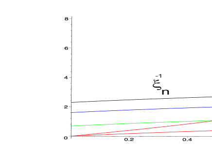
Figure 2: (Color Online) The longitudinal and transverse correlation lengths of matrix product states 43, as a function of the parameter $x$ for different values of the parameter $\mu:=\frac{2|ab|}{a^{2}+b^{2}}$. At $\mu=1$ both the transverse and longitudinal correlation lengths diverge at $x=0$.

An interesting point about transverse correlation functions is that depending on the sign of $\epsilon$, it becomes identically zero, on one side of the $g-$ axis and different from zero on the other side. Thus if one insists on a definition of an order parameter to be zero in one phase and non-zero in the other, then we can safely say that in these models, the transverse correlation function is an order parameter which signals a quantum phase transition.

Let us see study some limiting cases in these general models. At the point of phase transition $g=0$, as seen from (46), the state of a rung becomes a mixture of spin-zero states, and the two spins of a rung become fully anti-correlated in the $z$ direction, a fact which is reflected in (49). Near this point the correlation length $\xi_{z}$ becomes very large as seen from (57), although the amplitude becomes small since it is proportional to $|g|$. Thus at $g=0$ there is no long-range order in the model. Also from (54) and (51) it is readily seen that at $g=0$, the concurrence (or entanglement) of the two spins of a rung becomes maximum and equal to

$$C(g=0)=\frac{2|ab|}{a^{2}+b^{2}}.$$ (60)

On the other hand from (52) we see that as we approach the point $g=0$ from both sides, the von-Neumann entropy decreases. In addition, the derivative of both types of entanglement become singular at $g=0$. These facts show that the point of phase transition in these systems, is a point where the spins of a rung become highly entangled with each other and each rung becomes only slightly entangled to the rest of the lattice.
We can also obtain the explicit form of the state in this limit. From (43), and (2) we see that in this limit, no two spins in a rung can be in a $\left(\begin{array}[]{c}0\\ 0\end{array}\right)$ state. A little reflection shows that they can not be in the state $\left(\begin{array}[]{c}1\\ 1\end{array}\right)$ either, since in the absence of $A_{00}$, the only string of matrices with non-zero trace is a string of matrices $A_{01}$ and $A_{10}$ in arbitrary order. Since these matrices commute with each other, the resulting state has a simple description. Define two local states of a rung as

$$|u\rangle:=\left(\begin{array}[]{c}0\\ 1\end{array}\right)\equiv\left(\begin{array}[]{c}+\\ -\end{array}\right),\hskip 28.45274pt|d\rangle:=\left(\begin{array}[]{c}1\\ 0\end{array}\right)\equiv\left(\begin{array}[]{c}-\\ +\end{array}\right),$$ (61)

where for convenience we have re-introduced the spin notations $+$ and $-$ instead of qubit notation $0$ and $1$. Define a global un-normalized state $|u^{k},d^{N-k}\rangle$ to be the equally weighted linear combination of all states with $k$ local $u$ states and $N-k$ local $d$ state. Then from (43) and (2) we find that the ground state of the chain in the limit $g=0$ is given by

$$|\Psi\rangle=\frac{1}{\sqrt{Z}}\sum_{k=0}^{N}\left[a^{k}(\epsilon b)^{N-k}+b^{k}(\epsilon a)^{N-k}\right]|u^{k},d^{N-k}\rangle,$$ (62)

where $Z$ is the normalization constant given by

$$Z=\sum_{k=0}^{N}\left(\begin{array}[]{c}N\\ k\end{array}\right)\left[a^{k}(\epsilon b)^{N-k}+b^{k}(\epsilon a)^{N-k}\right]^{2}=2\left[(a^{2}+b^{2})^{N}+(2ab)^{N}\right].$$ (63)

At the other extreme when $|g|\rightarrow\infty$, the state of each rung becomes a mixture of fully aligned spins either in the positive or negative $z$ direction. This is also reflected in (49). In this limit a rung becomes entangled with the rest of the lattice, sine $\lim_{|g|\rightarrow\infty}S(\rho)=1$ and the two spins of a rung become disentangled from each other since $C=0$.
The explicit form of the state can also be obtained in this limit. In this case the only strings of matrices with non-vanishing traces are strings of $A_{00}$ and $A_{11}$ in alternating order. Thus if we define two local states

$$|t_{1}\rangle:=\left(\begin{array}[]{c}0\\ 0\end{array}\right)\equiv\left(\begin{array}[]{c}+\\ +\end{array}\right),\hskip 28.45274pt|t_{-1}\rangle:=\left(\begin{array}[]{c}1\\ 1\end{array}\right)\equiv\left(\begin{array}[]{c}-\\ -\end{array}\right),$$ (64)

then the ground state in this limit will be a GHZ state

$$|\Psi\rangle=\frac{1}{\sqrt{2}}(|t_{1},t_{1},\cdots,t_{1},t_{1}\rangle+|t_{-1},t_{-1},\cdots,t_{-1},t_{-1}\rangle).$$ (65)

In the next subsection we specialize these results to the two classes we discussed in the beginning of this subsection.

IV.1 Class A

This is the class which has the SO(2) symmetry (rotation around the $z$ axis in spin space) and three $Z_{2}$ symmetries (spin flip, parity, leg exchange). For this class we have from (32) that $b=\sigma a$. The parameter $x$ defined after equation (59) becomes equal to

$$x:=\frac{g}{2a^{2}}.$$ (66)

Insertion of $b=\sigma a$ in various quantities of the previous subsection shows that all the quantities can be expressed as a function of $x$, namely we find

$$\langle\sigma_{z}^{(1)}\sigma_{z}^{(2)}\rangle=\frac{|x|-1}{|x|+1},\hskip 28.45274pt\langle\sigma_{\bf n}^{(1)}\sigma_{\bf n}^{(2)}\rangle=\frac{\epsilon\sigma}{|x|+1},$$ (67)

$$\langle S_{z,1}S_{z,r}\rangle=-x^{2}\frac{(1-|x|)^{r-2}}{(1+|x|)^{r}},\hskip 28.45274pt\xi_{z}=\frac{1}{\ln(\frac{1+|x|}{1-|x|})},$$ (68)

and

$$\langle S_{{\bf n},1}S_{{\bf n},r}\rangle=(1+\epsilon\ sgn(x))(1+\sigma\ sgn(x))|x|\frac{\sigma^{r}}{(1+|x|)^{r}},\hskip 28.45274pt\xi_{\bf n}=\frac{1}{\ln(1+|x|)}.$$ (69)

We also find

$$S=\frac{|x|}{1+|x|}(1-\log|x|)+\log(1+|x|),$$ (70)

and

$$C=max(0,\frac{1-|x|}{1+|x|}).$$ (71)

Figure (2) show the entropy and the concurrence of the state of a single rung for this model.

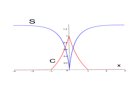
Figure 3: (Color Online) The von Neumann entropy of one single rung and its concurrence in models A, as functions of the parameter $x:=\frac{g}{2a^{2}}$, which is taken to be dimensionless.

IV.2 Class B

This is the class which has full SO(3) symmetry (rotation in spin space) and one discrete symmetry (spin flip) for generic values of $u$ and all the three $Z_{2}$ symmetries for $u=0$. For this class we have from (41) $g=\epsilon=-1$, $a=\frac{u+1}{2}$ and $b=\frac{u-1}{2}$. Inserting these values in the equations of the previous section we find the following:

$$\langle\sigma_{\bf n}^{(1)}\sigma_{\bf n}^{(2)}\rangle=\frac{1-u^{2}}{3+u^{2}},$$ (72)

and

$$\langle S_{{\bf n},1}S_{{\bf n},r}\rangle=-4\frac{(u^{2}-1)^{r-2}}{(u^{2}+3)^{r}},$$ (73)

where ${\bf n}$ is any direction in the spin space. The eigenvalues of the one-rung density matrix (51) in this case will be

$$\alpha_{1}=\alpha_{2}=\alpha_{3}=\frac{1}{u^{2}+3},\ \ \ \alpha_{4}=\frac{u^{2}}{u^{2}+3}.$$ (74)

Thus we find

$$S=\log(u^{2}+3)-\frac{u^{2}\log u^{2}}{u^{2}+3},$$ (75)

and

$$C=max(0,\frac{u^{2}-3}{u^{2}+3}).$$ (76)

Figure (3) show the entropy and the concurrence of the state of a single rung for this model.

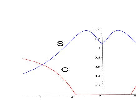
Figure 4: (Color Online)The von Neumann entropy of one single rung and its concurrence in model B as functions of the parameter $u$, which is taken to be dimensionless.

V Discussion

Although ladders of spin 3/2 models has already been studied in the context of vertex state models in mpswork3 , in which the ground state is constructed by a suitable concatenation of vertices assigned to single sites, the method developed in this work, in which each single rung is considered as a single site in a hyper-chain and the ground state is constructed as a matrix product state seems to us as more powerful and very easy to generalize to other spin models. In this work we have applied the matrix product formalism for construction of models on spin $1/2$ ladders. These models have been constructed to have special discrete and or continuous symmetries and to display a quantum phase transition in a broad sense, that is displaying non-analytical behavior in their correlation functions. Naturally these non-analytical behavior can also be observed in the entanglement properties of pairs of spins in these models. This route can be followed to develop other models, e.g models with higher spins or alternating spins on the rungs, with alternating coupling constants, or next-nearest neighbor interactions. By exploiting higher dimensional matrices and having more free parameters at our disposal, we may be able to construct continuous families of models on spin ladders which have full rotational symmetry. In this article we have restricted ourselves to frustration-free Hamiltonians and MPS states with fixed-size. Relaxing this latter condition allows one to represent any state $|\psi\rangle\in{\mathbb{C}}^{d\times N}$ as a matrix product state vidal ; MPSrep and then one may be able to study more diverse kinds of phase transitions on spin ladders. These matters will be taken up in separate publications.

VI Acknowledgement

We would like to thank A. Langari for very valuable discussions and the members of the Quantum information group of Sharif University, specially S. Alipour and L. Memarzadeh for instructive comments.

VII Appendix

In this appendix we briefly discuss the derivation of the explicit form of the Hamiltonian in terms of local spin operators. For simplicity we consider models in class A. The Hamiltonian for models in class B, can be constructed along similar lines. As explained in the main text, the starting point is to solve the system of equations

$$\sum_{i,j,k,l=0}^{1}c_{ijkl}A_{ij}A_{kl}=0.$$ (77)

This solution space is 12 dimensional since we have 4 equations for 16 unknowns. Thus we should find a set of 12 orthogonal vectors which span this solution space and then form a non-negative linear combination of the corresponding one dimensional projectors. The Hamiltonian constructed in this way does not necessarily have the symmetries imposed on the state, unless we choose new linear combinations of these vectors which transform suitably under the symmetry operators. These new basis vectors are found to be:

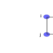
Figure 5: (Color Online) The labeling of the sites in equation (77), for the coefficients $c_{ijkl}$ and the corresponding states $|i\ j\ k\ l\rangle$.

$$|2,2\rangle := |0000\rangle$$ (78)

$$|2,1\rangle := \frac{1}{2}\left[-\epsilon|0001\rangle+|0010\rangle-\epsilon|0100\rangle+|1000\rangle\right]$$ (79)

$$|2,0\rangle := \frac{1}{\sqrt{6}}\left[-{4a^{2}}(|0011\rangle+|1100\rangle)+g\left(|0101\rangle+\sigma\epsilon|0110\rangle+\sigma\epsilon|1001\rangle+|1010\rangle\right)\right]$$ (80)

$$|1,1\rangle := \frac{1}{2}\left[\epsilon|0001\rangle+|0010\rangle-\epsilon|0100\rangle-|1000\rangle\right]$$ (82)

$$|1,0\rangle := \frac{1}{\sqrt{2}}\left[|0110\rangle-|1001\rangle\right]$$ (83)

$$|1^{\prime},1\rangle := \frac{1}{2}\left[-\sigma\epsilon|0001\rangle+|0010\rangle+\epsilon|0100\rangle-\sigma|1000\rangle\right]$$ (85)

$$|1^{\prime},0\rangle := \frac{1}{\sqrt{2}}\left[|0101\rangle-|1010\rangle\right]$$ (86)

$$|0,0\rangle := \frac{1}{2}\left[|0101\rangle-\sigma\epsilon|0110\rangle-\sigma\epsilon|1001\rangle+|1010\rangle\right],$$ (88)

with $|{\it l},-{\it m}\rangle=\sigma_{x}^{\otimes}|{\it l},{\it m}\rangle,\ \ \forall\ \ {\it l},{\it m}.$

Here we have organized the states in multiplets, with a labeling reminiscent of the one used in labeling the states of $so(3)$ representations. The reason is that in a certain limit ($\epsilon=\sigma=g=-1,a=\frac{1}{2}$) these states actually comprise the irreducible representations of $so(3)$ which emerge from the decomposition of the product of four spin one-half representations living on the sites of two rungs of the ladder. In fact for the product of these spin 1/2 representations we have

$$(\frac{1}{2})^{\otimes 4}=2\oplus 1\oplus 1^{\prime}\oplus 1"\oplus 0\oplus 0^{\prime}.$$

However only the representations $2,1,1^{\prime}$ and $0$ span the solution space of (77) in this limit. This labeling is useful because we can see under what conditions, the Hamiltonian become fully rotational invariant. Note also that we have used the labeling $|i\ j\ k\ l\rangle$ in accordance with the labeling of (77) for $c_{ijkl}$ (see figure (5). The reader can easily check that each of the above states (or more precisely the corresponding one dimensional projector) is invariant under the parity operation $\Pi:\ |i\ j\ k\ l\rangle\rightarrow|k\ l\ i\ j\rangle$ and leg-exchange of the ladder $Y:\ |i\ j\ k\ l\rangle\rightarrow|j\ i\ l\ k\rangle$. They also transform to each other under the spin-flip operation $X:\ |i\ j\ k\ l\rangle\rightarrow|\overline{i}\ \overline{j}\ \overline{k}\ \overline{l}\rangle$.

The local Hamiltonian which has the three discrete symmetries mentioned in the text and the symmetry around rotation along the $z$ axis in spin space, is constructed as follows:

$$h=\sum_{l=2,1,1^{\prime},0}\ \sum_{m=0}^{l}\mu_{lm}(|l,m\rangle\langle l,m|+|l,-m\rangle\langle l,-m|),$$ (89)

where the coefficients $\mu_{l,m}$ are non-negative parameters and together with the parameters $a$ and $g$ form the 10 free parameters of the Hamiltonian. Of course the total number of coupling constants (interaction strength) is 8, since we can always shift the ground state energy and also set the scale of energy by redefintion of these parameters. Re-expressing the local operators in terms of Pauli spin operators and rearranging terms, we find, after a rather lengthy calculation, the Hamiltonian acting on the ladder where we have multiplied $h$ by a factor of $8$ for convenience, (see figure (6) for labeling of sites of the ladder). Note that we use $z_{i}$ as an abbreviation to denote the operator $\sigma_{i,z}$ in the following. The total Hamiltonian is then given by

$$H=H_{1}+H_{2}+H^{(s)}_{1,2}+H^{z}_{1,2}+H^{(s,z)}_{1,2}$$ (90)

where

$$H_{1} = \sum_{i}J_{0}+J_{1}\ z_{i}z_{i+1}+J_{2}\ {\boldsymbol{\sigma}}_{i}\cdot{\boldsymbol{\sigma}}_{i+1}$$ (91)

$$H_{2} = \sum_{i}J_{0}+J_{1}\ z_{i^{\prime}}z_{i^{\prime}+1}+J_{2}\ {\boldsymbol{\sigma}}_{i^{\prime}}\cdot{\boldsymbol{\sigma}}_{i^{\prime}+1},$$ (92)

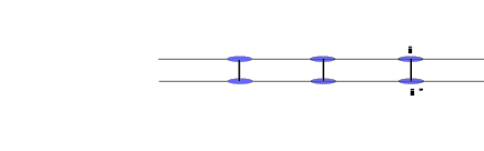
Figure 6: (Color Online) The labeling of sites of the ladder for reading the interaction terms in the Hamiltonian.

$$H^{(z)}_{12}=\sum_{i}J_{8}\ z_{i}z_{i^{\prime}}+J_{9}\ \left(z_{i}z_{i^{\prime}+1}+z_{i^{\prime}}z_{i+1}\right)+J_{10}\ z_{i}z_{i^{\prime}}z_{i+1}z_{i^{\prime}+1},$$

$$H^{(s)}_{12}=\sum_{i} J_{3} \ {\boldsymbol{\sigma}}_{i}\cdot{\boldsymbol{\sigma}}_{i^{\prime}}+J_{4}\ ({\boldsymbol{\sigma}}_{i}\cdot{\boldsymbol{\sigma}}_{i^{\prime}+1}+{\boldsymbol{\sigma}}_{i^{\prime}}\cdot{\boldsymbol{\sigma}}_{i+1})+J_{5}\ ({\boldsymbol{\sigma}}_{i}\cdot{\boldsymbol{\sigma}}_{i^{\prime}})({\boldsymbol{\sigma}}_{i+1}\cdot{\boldsymbol{\sigma}}_{i^{\prime}+1})$$

$$+ J_{6} \ ({\boldsymbol{\sigma}}_{i}\cdot{\boldsymbol{\sigma}}_{i+1})({\boldsymbol{\sigma}}_{i^{\prime}}\cdot{\boldsymbol{\sigma}}_{i^{\prime}+1})+J_{7}({\boldsymbol{\sigma}}_{i}\cdot{\boldsymbol{\sigma}}_{i^{\prime}+1})({\boldsymbol{\sigma}}_{i^{\prime}}\cdot{\boldsymbol{\sigma}}_{i+1}),$$ (93)

and

$$H^{(z,s)}_{12}=\sum_{i} J_{11} \left(z_{i}z_{i^{\prime}}({\boldsymbol{\sigma}}_{i+1}\cdot{\boldsymbol{\sigma}}_{i^{\prime}+1})+z_{i+1}z_{i^{\prime}+1}({\boldsymbol{\sigma}}_{i}\cdot{\boldsymbol{\sigma}}_{i^{\prime}})\right)$$

$$+ J_{12} \left(z_{i}z_{i+1}({\boldsymbol{\sigma}}_{i^{\prime}}\cdot{\boldsymbol{\sigma}}_{i^{\prime}+1})+z_{i^{\prime}}z_{i^{\prime}+1}({\boldsymbol{\sigma}}_{i}\cdot{\boldsymbol{\sigma}}_{i+1})\right)$$ (94)

$$+ J_{13} \left(z_{i}z_{i^{\prime}+1}({\boldsymbol{\sigma}}_{i}\cdot{\boldsymbol{\sigma}}_{i+1})+z_{i^{\prime}}z_{i+1}({\boldsymbol{\sigma}}_{i}\cdot{\boldsymbol{\sigma}}_{i^{\prime}+1})\right).$$ (95)

Thus there are bond interaction and plaquette interaction in the Hamiltonian all depending on 10 parameters. The coupling constants are related to these parameters as follows:

$$J_{0} = \mu_{22}+4(\mu_{21}+\mu_{11}+\mu_{1^{\prime}1})+\mu_{10}-\mu_{1^{\prime}0}+2(\mu_{00}+\mu_{20})+16a^{4}\mu_{20}$$

$$J_{1} = \mu_{22}+\frac{1}{2}(-\mu_{21}+\mu_{11}+\sigma\mu_{1^{\prime}1}+\mu_{1^{\prime}0}-\mu_{10})+\frac{4}{3}a^{2}(g\sigma\epsilon-2a^{2})\mu_{20}$$ (96)

$$J_{2} = \frac{1}{2}(\mu_{21}-\mu_{11}-\sigma\mu_{1^{\prime},1})-\frac{4}{3}\sigma\epsilon a^{2}g\mu_{20}$$ (97)

$$J_{3} = -\epsilon(\mu_{21}-\mu_{11})-\sigma\epsilon\mu_{1^{\prime}1}+\epsilon\sigma(\frac{2}{3}g^{2}\mu_{20}-\mu_{00})$$ (98)

$$J_{4} = -\frac{1}{2}\epsilon(\mu_{21}+\mu_{11}-\mu_{1^{\prime}1})-\frac{4}{3}a^{2}g\mu_{20}$$ (99)

$$J_{5} = \frac{1}{2}(\mu_{00}-\mu_{10}-\mu_{1^{\prime}0})+\frac{1}{3}\mu_{20}(g^{2}-8a^{4})$$ (100)

$$J_{6} = \frac{8}{3}a^{4}\mu_{20}+\frac{1}{2}(\mu_{1^{\prime}0}-\mu_{10})$$ (101)

$$J_{7} = \frac{8}{3}a^{4}\mu_{20}+\frac{1}{2}(\mu_{10}-\mu_{1^{\prime}0})$$ (102)

$$J_{8} = 2\mu_{22}+\epsilon(\mu_{21}-\mu_{11})+\sigma\epsilon\mu_{1^{\prime}1}-\mu_{10}-\mu_{1^{\prime}0}+(\sigma\epsilon-1)\mu_{00}+\frac{2}{3}\mu_{20}(8a^{4}-(1+\sigma\epsilon)g^{2})$$ (103)

$$J_{9} = \mu_{22}+\frac{1}{2}\epsilon(\mu_{21}+\mu_{11}-\mu_{1^{\prime}1})+\frac{1}{2}(\mu_{10}-\mu_{1^{\prime}0})+\frac{4}{3}a^{2}(g-2a^{2})\mu_{20}$$ (104)

$$J_{10} = \mu_{22}+2(\epsilon-1)\mu_{21}+(\epsilon+1)(\sigma-1)\mu_{1^{\prime}1}+(1-\sigma\epsilon)\mu_{00}+\frac{2}{3}(1+\sigma\epsilon)g^{2}\mu_{20}+\frac{8}{3}a^{2}(2a^{2}-g-g\sigma\epsilon)\mu_{20}$$ (105)

$$J_{11} = \frac{1}{2}(-\epsilon\mu_{21}+\epsilon\mu_{11}-\epsilon\sigma\mu_{1^{\prime}1}+\mu_{10}+\mu_{1^{\prime}0})+\frac{1}{2}(\epsilon\sigma-1)\mu_{00}+\frac{\mu_{20}}{3}(8a^{4}-(1+\sigma\epsilon)g^{2})$$ (106)

$$J_{12} = \frac{1}{2}(\mu_{21}-\mu_{11}-\sigma\mu_{1^{\prime}1}+\mu_{10}-\mu_{1^{\prime}0})-\frac{4}{3}a^{2}(2a^{2}-g\sigma\epsilon)\mu_{20}$$ (107)

$$J_{13} = \frac{1}{2}(-\epsilon\mu_{21}-\epsilon\mu_{11}+\epsilon\mu_{1^{\prime}1}-\mu_{10}+\mu_{1^{\prime}0})+\frac{4}{3}a^{2}\mu_{20}(g-2a^{2}).$$ (108)

This is a complicated looking Hamiltonian, with many types of interactions, but in view of the large number of parameters, it is possible to look at specific subsets of the parameter space, where some of the interactions are absent. Indeed the parameter space consists of four disconnected parts, each of which corresponds to one choice of the pair $(\sigma,\epsilon)$. Let us for example consider the subset on which the Hamiltonian has full rotational symmetry. It is well known that any operator of the form $\sum_{m=-l}^{l}|l,m\rangle\langle l,m|$ is a scalar. Thus in the limit $g=\epsilon=\sigma=-1,a=\frac{1}{2}$ if we set $\mu_{2m}=:6\mu,\ \mu_{1,m}=:2\nu,\ \mu_{1^{\prime},m}=:2\xi\ \ \ \forall\ \ m$ and $\mu_{0,0}=:2\eta$, then we will have a Hamiltonian which is fully rotational invariant. On can see that in this limit, all the coupling constant corresponding to non-scalar terms in the Hamiltonian vanish and we are left with

$$J_{0} = 48\mu+10\nu+6\xi+4\mu$$

$$J_{2} = 5\mu-\nu+\xi$$ (109)

$$J_{3} = 10\mu-2\nu-2\xi-2\eta$$ (110)

$$J_{4} = 5\mu+\nu-\xi$$ (111)

$$J_{5} = \mu-\nu-\xi+\eta$$ (112)

$$J_{6} = \mu+\xi-\nu$$ (113)

$$J_{7} = \mu+\nu-\xi.$$ (114)

References

• (1) S. Sachdev, Quantum Phase Transitions (Cambridge University Press, Cambridge, 1999).
• (2) A. Osterloh, L. Amico, G. Falci, and R. Fazio, Nature 416, 608 (2002).
• (3) T. Osborne, M. Nielsen, Phys. Rev. A, 66, 032110 (2002).
• (4) M. C. Arnesen, S. Bose, and V. Vedral, Phys. Rev. Lett. 87, 277901 (2001); D. Gunlycke et al, Phys. Rev. A 64, 042302 (2001).
• (5) S. Hill and W. K. Wootters, Phys. Rev. Lett. 78, 5022 (1997); W. K. Wootters, Phys. Rev. Letts. 80, 2245 (1998).
• (6) A. Klumper, A. Schadschneider and J. Zittartz, J. Phys. A (1991) L293; Z. Phys. B, 87 (1992) 281; Europhys. Lett., 24 (1993) 293.
• (7) M. Fannes, B. Nachtergaele and R. F. Werner, Commun. Math. Phys. 144, 443 (1992).
• (8) M. M. Wolf, G. Ortiz, F. Verstraete and I. Cirac, Phys. Rev. Lett. 97, 110403 (2006).
• (9) D. Peres Garcia, et al, quant-ph/0608197.
• (10) M. A. Ahrens, A. Schadschneider, and J. Zittartz, Europhys. Lett. 59 6, 889 (2002).
• (11) E. Bartel, A. Schadschneider and J. Zittartz, Eur. Phys. Jour. B, 31, 2, 209-216 (2003).
• (12) H. Niggemann, and J. Zittartz, J. Phys. A: Math. Gen. 31, 9819-9828 (1998).
• (13) F. Verstraete, D. Porras, J. I. Cirac, Phys. Rev. Lett. 93, 227205 (2004).
• (14) F. Verstraete, J. J. Garcia-Ripoll, and J. I. Cirac, Phys. Rev. Lett. 93, 207204 (2004).
• (15) F. Verstraete, J. I. Cirac, Phys. Rev. B 73, 094423 (2006); T. J. Osborne, Phys. Rev. Lett. 97, 157202 (2006); M. B. Hastings, Phys. Rev. B 73, 085115 (2006).
• (16) G. Vidal, Phys. Rev. Lett. 91, 147902 (2003).
• (17) A. K. Kolezhuk and H. J. Mikeska, Phys. Rev. Lett. 80, 2709 (1998); Int. J. Mod. Phys. B, Vol.12, 2325-2348 (1998).