Superseded version of the WKB approximation and explanation of emergence of classicality

Abstract

Regarding the limit $\hbar\rightarrow 0$ as the classical limit of quantum mechanics seems to be silly because $\hbar$ is a definite constant of physics, but it was successfully used in the derivation of the WKB approximation. A superseded version of the WKB approximation is proposed in the classical limit $\alpha\rightarrow 0$ where $\alpha=m/M$ is the screening parameter of an object in which m is the mass of the effective screening layer and M the total mass. This version is applicable to not only approximate solution of Schrödinger equation of a quantum particle but also that of a nanoparticle. Moreover, the version shows that the quantization rules for nanoparticles can be achieved by substituting $\alpha\hbar$ for $\hbar$ in the Bohr-Sommerfeld quantization rules of the old quantum theory. Most importantly, the version helps clarify the essential difference between classical and quantum realities and understand the transition from quantum to classical mechanics as well as quantum mechanics itself.

1 Introduction

The WKB (Wentzel-Kramers-Brillouin) approximation or phase-integral approximation plays an important role in the solution of Schrödinger equation in the case where a particle has low momentum and moves through a slowly varying potential and in the proof of the Bohr-Sommerfeld quantization rules.[1-3] This approximation method is based on the limit $\hbar\rightarrow 0$ which was first considered as the classical limit of quantum theory by Max Planck who stated:$``$The classical theory can simply be characterized by the fact that the quantum of action becomes infinitesimally small.$"$[4] However, the fact that the diffraction and interference of, for example, the grains of sand do not really occur when they pass through slits can be properly explained by considering that the outer matter of a tiny grain of sand screens nearly completely the associated wave by the inner matter.[5] This proposed screening effect gives a logical description of transition from a quantum particle to a classical object and gives a general momentum-position uncertainty relation [6]:

$$\triangle p_{x}^{(\alpha)}\triangle x=\alpha\triangle p_{x}\triangle x\geq\frac{\alpha\hbar}{2},\mbox{ }1\geq\alpha>0$$ (1)

where $\alpha$ is the screening mass parameter defined by $\alpha=m/M$ in which m is the mass of the effective screening layer and M the total mass. For a spherical nanoparticle shown in Fig.1, the corresponding screening size parameter is $\sigma=r_{m}/r_{M}=1-(1-\alpha)^{1/3}$ [6]. The thickness of the effective screening layer having quantum behavior is estimated to be a few nanometers.

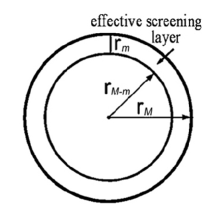
Figure 1: Sketch of the effective screening layer in a spherical nanoparticle.

Obviously the Heisenberg uncertainty relation is only applicable to quantum particles ($\alpha$=1), but not applicable to macroscopic objects ($\alpha\rightarrow 0$) and mesoscopic objects (between). The fact that the momentum and position of a macroscopic object are measurable simultaneously with finite errors implies the limit $\alpha\rightarrow 0$ instead of the formal limit $\hbar\rightarrow 0$. It seems to be silly to regard the universal fundamental physical constant $\hbar$ as a variable quantity. We will thus propose a superseded version of the WKB approximation in the classical limit $\alpha\rightarrow 0$. This limit is proper and general, which, as will be seen below, corresponds to the emergence of classicality from quantum mechanics.

2 Superseded version of the WKB approximation

Traditionally, the wave function in the WKB approximation is expanded in terms of $\hbar$, which is based on the Planck limit $\hbar\rightarrow 0$. Indeed, $\hbar=1.05457\times 10^{-34}$ Joule-sec and the Planck limit has no physical interpretation. Now, using the limit $\alpha\rightarrow 0$ instead of the Planck limit for derivation of the approximation, we assume that the Schrödinger equation of an object with an effective screening parameter $\alpha$ moving through a one-dimensional potential $V(x)$ is expressed by

$$\frac{\mbox{d}^{2}\psi}{\mbox{d }x^{2}}+\frac{2M}{\alpha^{2}\hbar^{2}}(E-V)\psi=0$$ (2)

where $1\geq\alpha>0$. This equation implies that the momentum operator now is $-i\alpha\hbar\partial/\partial x$ ($-i\alpha\hbar\nabla$ in 3 dimensions). Of course the energy operator correspondingly becomes $i\alpha\hbar\partial/\partial t$. The equation also implies that the commutator $[\hat{x},\hat{p}]=i\alpha\hbar\{x,p\}=i\alpha\hbar$ in which $\{x,p\}$ is the Poisson bracket of x and p and that the Bohm quantum potential [7] approaches 0 when $\alpha\rightarrow 0$ instead of $\hbar\rightarrow 0$. The approximate solution of the equation can be written in the form:

$$\psi=\exp(\frac{i}{\alpha\hbar}\int^{x}y\mbox{d}x),\mbox{ }y=y(x,\alpha)$$ (3)

which satisfies

$$(-\frac{y^{2}}{\alpha^{2}\hbar^{2}})\psi+(\frac{i}{\alpha\hbar})y^{\prime}\psi+\frac{2M}{\alpha^{2}\hbar^{2}}(E-V)\psi=0$$ (4)

where the prime denotes differentiation with respect to x. So, assuming $\psi\neq 0$, we obtain

$$(\frac{\alpha\hbar}{i})y^{\prime}=p^{2}-y^{2},\mbox{ }p^{2}=2M(E-V)$$ (5)

We now expand $y$ as a series in powers of $\alpha/i$:

$$y=y_{0}+(\frac{\alpha}{i})y_{1}+(\frac{\alpha}{i})^{2}y_{2}+\cdots,\mbox{ }1\geq\alpha>0$$ (6)

Therefore we have

$$(\frac{\alpha\hbar}{i})y^{\prime}=(\frac{\alpha\hbar}{i})\sum^{\infty}_{n=0}(\frac{\alpha}{i})^{n}y^{\prime}_{n}$$ (7)

$$p^{2}-y^{2}=p^{2}-\sum^{\infty}_{l,m=0}(\frac{\alpha}{i})^{l+m}y_{l}y_{m}$$ (8)

Thus Eq.5 becomes

$$\hbar\sum^{\infty}_{n=1}(\frac{\alpha}{i})^{n}y^{\prime}_{n-1}=p^{2}-\sum^{\infty}_{l,m=0}(\frac{\alpha}{i})^{l+m}y_{l}y_{m}$$ (9)

Equating coefficients of the same powers of $\alpha/i$ on the left and right sides of the above equation, we get

$$y_{0}=\pm p=\pm\sqrt{2M(E-V)}$$ (10)

$$\hbar y^{\prime}_{n-1}=-\sum^{n}_{m=0}y_{n-m}y_{m},\mbox{ }n=1,2,3,\cdots$$ (11)

From Eq.10 and Eq.11 we have

$$y^{\prime}_{0}=\pm\frac{1}{2}\cdot\frac{-2MV^{\prime}}{\sqrt{2M(E-V)}}=-\frac{MV^{\prime}}{y_{0}}$$ (12)

$$\hbar y^{\prime}_{0}=-2y_{1}y_{0}$$ (13)

and hence get

$$y_{1}=\frac{\hbar V^{\prime}}{4(E-V)}$$ (14)

Furthermore, we have the equations

$$\hbar y^{\prime}_{1}=-y^{2}_{1}-2y_{0}y_{2}$$ (15)

$$y^{\prime}_{1}=\frac{\hbar}{4}\cdot\frac{V^{\prime\prime}(E-V)+V^{\prime 2}}{(E-V)^{2}}$$ (16)

and hence obtain

$$y_{2}=\frac{1}{2y_{0}}(-y^{2}_{1}-\hbar y^{\prime}_{1})=\mp\frac{\hbar^{2}}{32}\cdot\frac{5V^{\prime 2}+4V^{\prime\prime}(E-V)}{(2M)^{1/2}(E-V)^{5/2}}$$ (17)

Similarly from

$$\hbar y^{\prime}_{2}=-2y_{3}y_{0}-2y_{2}y_{1}$$ (18)

it follows that

$$y_{3}=\frac{1}{2y_{0}}(-\hbar y^{\prime}_{2}-2y_{2}y_{1})=-\hbar\frac{\mbox{d}}{\mbox{d}x}(\frac{y_{2}}{2y_{0}})$$ (19)

And similarly for higher terms in $\alpha/i$. Now we write the power series as follows

$$y(x,\alpha)=\pm\sqrt{2M(E-V)}+(\frac{\alpha}{i})\frac{\hbar V^{\prime}}{4(E-V)}$$

$$\mp(\frac{\alpha}{i})^{2}(\frac{\hbar^{2}}{32}\cdot\frac{5V^{\prime 2}+4V^{\prime\prime}(E-V)}{(2M)^{1/2}(E-V)^{5/2}})+\cdots$$ (20)

This formulas is the same as that obtained from the original version of the WKB approximation when $\alpha=1$. Evidently, this superseded version is general in the sense that it is applicable to not only quantum particles ($\alpha=1$) but also nanoparticles ($1>\alpha>0$).

As well known, usually it is only necessary to take the first two terms of the above series. By using the equation

$$\int^{x}\frac{V^{\prime}}{4(E-V)}\mbox{d}x=-\frac{1}{2}\log p$$ (21)

we can thus write

$$\psi=\frac{C_{1}}{\sqrt{p}}\exp(\frac{i}{\alpha\hbar}\int^{x}p\mbox{d}x)+\frac{C_{2}}{\sqrt{p}}\exp(-\frac{i}{\alpha\hbar}\int^{x}p\mbox{d}x),\mbox{ }p=\sqrt{2M(E-V)}$$ (22)

in which the coefficients $C_{1}$ and $C_{2}$ are determined by boundary and normalization conditions. The difficulty that rises is that the WKB approximation becomes inapplicable at the classical returning points where $E-V$=0, but the approximate wave functions near the points can be easily obtained from solving the Schrödinger equation and hence the connection formula between the WKB wave functions and the approximate wave functions can be derived in the way shown in many textbooks on quantum mechanics, such as that by Merzbacher [8]. This version shows that the quantization rules for nanoparticles can be achieved by substituting $\alpha\hbar$ for $\hbar$ in the Bohr-Sommerfeld quantization rules of the old quantum theory.

In order to investigate the relation between classical and quantum mechanics, we now write Eq.3 as the following form:

$$\psi=\exp(\frac{iS_{\alpha}}{\alpha\hbar}),\mbox{ }S_{\alpha}=\int^{x}y(x,\alpha)\mbox{d}x$$ (23)

Substituting this wave function into Eq.2 and assuming $\psi\neq 0$, we get

$$(\frac{\mbox{d }S_{\alpha}}{\mbox{d }x})^{2}+(\frac{\alpha\hbar}{i})\frac{\mbox{d}^{2}S_{\alpha}}{\mbox{d }x^{2}}-2M(E-V)=0$$ (24)

When $\alpha\rightarrow 0$, it becomes the well known Hamilton-Jacobi equation

$$(\frac{\mbox{d }S_{0}}{\mbox{d }x})^{2}-2M(E-V)=0$$ (25)

in which $S_{0}$ is the action function of classical mechanics, so the limit $\alpha\rightarrow 0$ corresponds to the emergence of classicality from quantum mechanics. This point is vital for understanding quantum mechanics.

3 Conclusion

A superseded version of the WKB approximation has been proposed in the classical limit $\alpha\rightarrow 0$ where $\alpha=m/M$ is the screening parameter of an object in which m is the mass of the effective screening layer and M the total mass. This version is applicable to not only approximate solution of Schrödinger equation of a quantum particle but also that of a nanoparticle. Moreover, the version shows that the quantization rules for nanoparticles can be achieved by substituting $\alpha\hbar$ for $\hbar$ in the Bohr-Sommerfeld quantization rules of the old quantum theory. Most importantly, the version helps clarify the essential difference between classical and quantum realities and understand the transition from quantum to classical mechanics as well as quantum mechanics itself.

References

- [1] Wentzel, G., Z. Physik 38, 518 (1926).
- [2] Kramers, H. A., Z. Physik 39, 828 (1926).
- [3] Brillouin, L., Comp. Rend. 183, 24 (1926).
- [4] Planck, M., The theory of heat radiation (1906), trans. by M. Masius (Dover, New York, 1959), p. 143.
- [5] Wang Guowen, Heuristic explanation of quantum interference experiments, quant-ph/0501148.
- [6] Wang Guowen, Finding way to bridge the gap between quantum and classical mechanics, physics/0512100.
- [7] Bohm, D., Phys. Rev. 85, 166 (1952).
- [8] Merzbacher, E., Quantum mechanics, 2nd ed. (Wiley, New York, 1970), chap. 7.