Pooling quantum states obtained by indirect measurements

Abstract

We consider the pooling of quantum states when Alice and Bob both have one part of a tripartite system and, on the basis of measurements on their respective parts, each infers a quantum state for the third part $S$. We denote the conditioned states which Alice and Bob assign to $S$ by $\alpha$ and $\beta$ respectively, while the unconditioned state of $S$ is $\rho$. The state assigned by an overseer, who has all the data available to Alice and Bob, is $\omega$. The pooler is told only $\alpha$, $\beta$, and $\rho$. We show that for certain classes of tripartite states, this information is enough for her to reconstruct $\omega$ by the formula $\omega\propto\alpha\rho^{-1}\beta$. Specifically, we identify two classes of states for which this pooling formula works: (i) all pure states for which the rank of $\rho$ is equal to the product of the ranks of the states of Alice’s and Bob’s subsystems; (ii) all mixtures of tripartite product states that are mutually orthogonal on $S$.

I Introduction

In the approach to quantum theory wherein a quantum state encodes an observer’s knowledge of a system, different observers may assign different quantum states.  It is then natural to ask which pairs of quantum states are compatible in the sense that they can be simultaneously assigned by a pair of observers BFM02 ; Bru02 . Another natural question concerns pooling Bru02 ; Jac02 ; PB03 ; Her04 ; Jac05 ; Bru06 : what is the quantum state that ought to be assigned to a system by someone who learns only the quantum states assigned to it by two distinct observers?

The way in which we have just posed the pooling problem — the standard way to do so — presumes that no further assumptions need to be specified in order for there to be a unique solution. That this is not necessarily the case becomes clear when we examine carefully the notion of pooling states of knowledge in classical probability theory. Such an analysis is particularly appropriate given that the problem of pooling quantum states was originally conceived as an analogue of classical pooling.

The classical pooling result may be stated in the following way. Suppose that Alice and Bob share a prior probability distribution $p(s)$ over a space of hypotheses. Suppose further that the data they acquire before updating their distributions is obtained independently. Specifically, if $a$ denotes Alice’s data and $b$ denotes Bob’s data, then these are assumed to be conditionally independent given $s$:

$$p(a,b|s)=p(a|s)p(b|s).$$ (1)

In these circumstances, Alice, upon learning $a$, updates her description from $p(s)$ to $p(s|a)\propto p(a|s)p(s)$ and Bob, upon learning $b$, updates his description from $p(s)$ to $p(s|b)\propto p(b|s)p(s)$. A third party who has access to both data $a$ and $b$, whom we shall call the overseer and name Oswald, would update his description from $p(s)$ to $p(s|a,b)$, where

$$p(s|a,b)\propto\frac{p(s|a)p(s|b)}{p(s)}\;,$$ (2)

as one easily verifies by applying Bayes’ theorem to Eq. (1). In fact, Eq. (2) holds only for those values of $s$ for which $p(s)>0$; for values of $s$ for which $p(s)=0$, Oswald assigns $p(s|a,b)=0$. The important point to note is that the overseer’s probability distribution depends only on the prior distribution and Alice’s and Bob’s posterior distributions. Thus, another party, who only has knowledge of these three distributions, can reconstruct Oswald’s distribution. This person, whom we shall call the pooler and name Penelope, need not know any additional details of how Alice and Bob came to update the prior in the way that they did.

However, the formula (2) does not hold in general, as discussed in Sec. II.2. In such cases, Oswald, who is aware of how the data was acquired, can still use Bayes’ theorem to update his distribution. But Penelope, who only has the prior distribution and Alice’s and Bob’s posterior distributions at her disposal, has insufficient information to reconstruct Oswald’s state of knowledge. It is only under special circumstances, such as when Eq. (1) holds, that she is able to do so.

The lessons of classical pooling for quantum pooling are several. First, we have seen that in the one case where the pooler can reconstruct the overseer’s posterior distribution, she must use not only Alice and Bob’s distributions, but also the prior distribution. Consequently, we expect that in the quantum case she will require not only Alice’s and Bob’s quantum states, but also the “prior” quantum state — the one that they both assigned prior to the measurements. Second, in order to tackle the pooling problem, it has been useful to imagine an overseer who knows every aspect of the protocol and the collected data, because his posterior is guaranteed to be uniquely specified by Bayes’ theorem. This suggests that in the quantum case, we again ought to consider an overseer of this nature, because the quantum state that the overseer must assign after the measurements — the “posterior” quantum state — will be uniquely specified by quantum theory (through the quantum update rule). If this state is a function only of Alice’s state, Bob’s state, and the prior state, then Penelope can succeed in her task of reconstruct Oswald’s posterior state. Third, we expect that there are limited circumstances in which the pooler can succeed in this fashion.

Most of the previous work on pooling has not taken this approach. Typically, the prior quantum state is not specified in the problem, nor is it specified how Alice and Bob acquired their data Bru02 ; PB03 ; Her04 ; the notion of pooling that is discussed in these papers is therefore distinct from the one considered here. On the other hand, Jacobs Jac02 ; Jac05 and Brun in Ref. Bru06 have emphasized the importance of the method of data acquisition for pooling knowledge about a system, have taken care to specify a prior quantum state (they both assume a completely mixed state), and have used the device of an overseer to evaluate pooling strategies. The pooling problem that Jacobs considers is nonetheless distinct from the one considered here. This is because the two states to be pooled in his approach are not simultaneous descriptions of a single system. Rather, they are descriptions of a single system at two times, between which there is an intervening direct measurement on the system, a measurement which may well invalidate the applicability of the earlier description . However, a particular instance of state pooling considered by Brun in Ref. Bru06 (wherein Alice and Bob obtain conditionally independent data about the outcome of a measurement on the system) does fall within the general framework described above.

In the present article, we consider the specific case where Alice’s and Bob’s data are obtained by measurements upon two different shares of a tripartite system prepared in a quantum state known to them both. Based upon this data, they calculate updated states for the third share. We identify two classes of tripartite states for which Alice’s and Bob’s updated states, together with their initial state (for this third share), enable Penelope to reconstruct Oswald’s state, in analogy to Eq. (2). This is illustrated in Fig. 1. We also show that our formula fails in more general cases, as one would expect. We discuss the relation of our results to state compatibility, and generalize our results to the case of arbitrarily many parties.

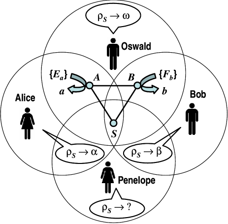
Figure 1: Schematic of the pooling problem we consider. All parties seek to update the quantum state they assign to system $S$ based on the information they acquire. Each party has access to only certain information, represented by the contents of the circle in which he or she is enclosed. All information about $S$ is ultimately derived from indirect measurements on $S$, that is, measurements upon systems ($A$ and $B$) that are correlated with $S$. The prior knowledge about $A$, $B$, and $S$ of the different parties derives from a single tripartite state, but each party has the reduced state for only those systems contained in his or her circle. Alice performs a measurement on $A$ (represented by a POVM $\{E_{a}\}$) with outcome $a$, and updates her state for $S$ to $\alpha$. Bob does likewise, mutatis mutandis. Oswald, the overseer, learns everything known to Alice and Bob and updates his state to $\omega$. Penelope, the pooler, learns only the manner in which Alice and Bob update their states. The question we address is: what state should she assign to $S$?

II Pooling quantum states from indirect measurements

The scenario we consider is as follows . There is a tripartite system $ABS$ for which Alice possesses the $A$ share and Bob possesses the $B$ share. They both initially describe the tripartite system by the (possibly mixed) quantum state $W$ defined on $\mathcal{H}^{A}\otimes\mathcal{H}^{B}\otimes\mathcal{H}^{S},$ and thus they both initially describe the third system $S$ by the same reduced state $\rho\equiv\text{Tr}_{AB}\left(W\right)$. Alice makes a generalized measurement on $A,$ and Bob makes a generalized measurement on $B.$ After registering the outcome of her measurement, Alice updates her description of the system $S$ to a new quantum state which we denote by $\alpha$. Likewise, after registering the outcome of his measurement, Bob updates his description of $S$ to a new quantum state which we denote by $\beta.$ Quantum theory uniquely specifies how Alice and Bob ought to update their descriptions. (Strictly speaking, Alice only requires the reduction of $W$ to $AS$ and Bob only requires the reduction to $BS$, as is indicated schematically in Fig. 1.)

The overseer, Oswald, knows everything there is to know: the initial state $W,$ what measurements Alice and Bob made, and the outcomes they obtained. After learning all of this information, the overseer updates his description of $S$ to the state $\omega.$ Again, quantum theory uniquely specifies how the overseer ought to update his description.

The pooler, Penelope, is not given any information about what measurements are made by Alice and Bob, nor their outcomes. Rather, she is told only the identity of the initial quantum state for $S$ as well as the quantum states that Alice and Bob assign to $S$ at the end of their measurements. In other words, the pooler is given only $\rho$, $\alpha$ and $\beta.$ Her task is to “pool” the information contained in $\alpha$ and $\beta$ (and possibly also $\rho$) to obtain a single quantum state that will represent what she predicts about the outcomes of future experiments on $S.$

By analogy with the classical case, we expect that the quantum pooling problem only has a solution when Alice’s and Bob’s data satisfy some condition of independence. Although we do not determine the most general condition here, we do illustrate two simple classes of states $W$ for which the quantum pooling problem can be solved. Class (i) is the class of pure tripartite states in which the rank of $\rho$ is maximal (in a sense defined below). Class (ii) is the class of mixtures of product states that are mutually orthogonal on $S$.

We show that for both classes, Oswald’s quantum state $\omega$ can be written as a simple function of $\alpha,$ $\beta$, and $\rho$, namely,

$$\omega \propto \alpha\rho^{-1}\beta$$ (3)

$$= \beta\rho^{-1}\alpha,$$ (4)

where $\rho^{-1}$ is the inverse of $\rho$ on its support . To obtain the precise form of $\omega$, one need only normalize the right-hand side of this expression. Penelope can obviously construct this state, and so for these classes, she succeeds in the pooling task.

II.1 Class (i)

Let $W\equiv|{\Psi}\rangle\langle{\Psi}|$, where $|{\Psi}\rangle$ is a tripartite state. We define $\mathcal{H}^{X}$ ($X=A,B,S$) to be the support of $W$ on subsystem $X$. That is, if $d_{X}$ is the rank of the reduced state of the subsystem $X$, this is also the dimensionality of $\mathcal{H}^{X}$. Now restrict to the class of pure states where $d_{S}=d_{A}d_{B}$. Note that this is the maximal value $d_{S}$ can take, given $d_{A}$ and $d_{B}$, because (from the purity of $W$) $d_{S}=d_{AB}\leq d_{A}d_{B}$. By the Choi-Jamiolkowski isomorphism Jam72 , any $|{\Psi}\rangle$ satisfying this condition can be written as

$$\left|\Psi\right\rangle=\sum_{e=1}^{d_{A}}\sum_{f=1}^{d_{B}}\left|e,f\right\rangle\otimes(\sqrt{\rho}\,U\left|e,f\right\rangle).$$ (5)

Here $\{\left|e,f\right\rangle\}$ is a complete orthonormal basis for $\mathcal{H}^{A}\otimes\mathcal{H}^{B}$, and $U$ is a unitary operator from $\mathcal{H}^{A}\otimes\mathcal{H}^{B}$ to ${\cal H}^{S}$, so that $U^{\dagger}U=I^{A}\otimes I^{B}$.

Alice’s generalized measurement can be represented by a positive-operator-valued-measure (POVM) $\left\{{E_{a}}\right\}$. If she gets result $a$ then the relevant POVM element (also called an effect) is the positive operator $E_{a}\otimes I\text{ on }\mathcal{H}^{A}\otimes\mathcal{H}^{B}.$ She updates her description of $S$ from $\rho$ to

$$\alpha \propto{\rm Tr}_{AB}[(E_{a}\otimes I)|{\Psi}\rangle\langle{\Psi}|]$$

$$=\sum_{e,f,e^{\prime},f^{\prime}}\langle e^{\prime},f^{\prime}|E_{a}\otimes I|e,f\rangle\sqrt{\rho}\,U\left|e,f\right\rangle\langle e^{\prime},f^{\prime}|U^{{\dagger}}\sqrt{\rho}\,$$

$$=\sqrt{\rho}\,U(E_{a}\otimes I)^{T}U^{\dagger}\sqrt{\rho}\,,$$ (6)

where $M^{T}$ denotes the transpose of $M$ in the basis $|{e,f}\rangle$ and where we have made use of the completeness of this basis. Note that the update rule for indirect measurements has the POVM element sandwiched between square roots of the state. This is the opposite of what occurs with direct measurements where the state is typically sandwiched between square roots of the POVM element. Equation (II.1) is an instance of the Hughston-Jozsa-Wootters theorem HJW93 generalized to POVM measurements Fuc02 ; SR02 . The trace of the right-hand-side of Eq. (II.1) is the probability for Alice to have obtained the result she did, and $\alpha$ is simply the right-hand-side divided by this quantity.

Similarly, if the POVM that Bob measures is $\left\{{F_{b}}\right\}$, the effect corresponding to the result $b$ is $I\otimes F_{b}\text{ on }\mathcal{H}^{A}\otimes\mathcal{H}^{B}.$ Then he updates his description of $S$ from $\rho$ to

$$\beta\propto\sqrt{\rho}\,U(I\otimes F_{b})^{T}U^{\dagger}\sqrt{\rho}.$$ (7)

The overseer, upon being told Alice’s and Bob’s outcomes, updates his description of $S$ from $\rho$ to

$$\omega\propto\sqrt{\rho}\,U(E_{a}\otimes F_{b})^{T}U^{\dagger}\sqrt{\rho}.$$ (8)

It follows from the above results that

$$\omega \propto\sqrt{\rho}\,U(I\otimes F_{b})^{T}(E_{a}\otimes I)^{T}U^{{\dagger}}\sqrt{\rho}$$

$$=\sqrt{\rho}\,U(I\otimes F_{b})^{T}U^{\dagger}U(E_{a}\otimes I)^{T}U^{\dagger}\sqrt{\rho}$$

$$=\sqrt{\rho}\,U(E_{a}\otimes I)^{T}U^{\dagger}\sqrt{\rho}\,\rho^{-1}\sqrt{\rho}\,U(I\otimes F_{b})^{T}U^{\dagger}\sqrt{\rho}$$

$$\propto\alpha\rho^{-1}\beta.$$ (9)

Here we have made use of the fact that $U^{\dagger}U$ is the identity operator on $\mathcal{H}^{A}\otimes\mathcal{H}^{B},$ the fact that $(AB)^{T}=B^{T}A^{T},$ and the fact that $\sqrt{\rho}\rho^{-1}\sqrt{\rho}$ is the identity operator on $\mathcal{H}^{S}$ (by virtue of the rank condition on $\rho$).

Thus we have shown that Penelope should pool the states according to Eq. (3). The proof of the second identity (4) is identical, except that the order of $(I\otimes F_{b})$ and $(E_{a}\otimes I)$ (which commute) is inverted in the first line of Eq. (9).

II.1.1 Example

To aid the reader’s understanding, we now give an explicit application of the above case. Consider the following state in $\mathcal{H}^{A}\otimes\mathcal{H}^{B}\otimes\mathcal{H}^{S}$:

$$|{\Psi}\rangle\propto|{0}\rangle|{0}\rangle|{0}\rangle+|{0}\rangle|{1}\rangle|{1}\rangle+|{1}\rangle|{0}\rangle|{2}\rangle+|{1}\rangle|{1}\rangle|{3}\rangle,$$ (10)

which satisfies the rank condition for class (i) states since $d_{S}=4$ and $d_{A}=d_{B}=2$. It is obvious that if Alice and Bob measure in the logical ($|{0}\rangle,|{1}\rangle$) basis then the pooling formula will hold, as each of them holds independent classical information about the logical state of $S$. It is less obvious that Eq. (3) holds regardless of the measurements they make.

Suppose, for example, that Alice and Bob both measure in the ($|{+}\rangle,|{-}\rangle$) basis, where $|{\pm}\rangle\propto|{0}\rangle\pm|{1}\rangle$. Say they both obtain the result $+$. Then it is easy to verify that Alice’s updated state for $S$ is

$$\alpha\propto\uplus\left({|{0}\rangle+|{2}\rangle}\right)\uplus\left({|{1}\rangle+|{3}\rangle}\right).$$ (11)

Here, following Ref. Jon06 , we are using the following notation, that for an arbitrary ray $|{r}\rangle$, we have $\uplus|{r}\rangle\equiv+|{r}\rangle\langle{r}|$. Similarly, Bob’s new state assignment is

$$\beta\propto\uplus\left({|{0}\rangle+|{1}\rangle}\right)\uplus\left({|{2}\rangle+|{3}\rangle}\right),$$ (12)

while Oswald’s state (which is pure) is

$$\omega\propto\uplus\left({|{0}\rangle+|{1}\rangle+|{2}\rangle+|{3}\rangle}\right).$$ (13)

Now for the state (10), $\rho\propto I$, from which it is easy to verify that Eq. (3) holds.

II.1.2 Pure states for which the pooling formula fails

If a pure state does not satisfy the rank condition for class (i) states, then in general the pooling formula does not hold. This can be seen from the Greenberger-Horne-Zeilinger state

$$|{\Psi}\rangle=|{0}\rangle|{0}\rangle|{0}\rangle+|{1}\rangle|{1}\rangle|{1}\rangle.$$ (14)

Here $d_{S}=d_{A}=d_{B}=2$ so that $d_{S}\neq d_{A}d_{B}$. As with state (10), if Alice and Bob both measure in the logical basis then the pooling formula will hold. But in contrast with state (10), this is no longer true if they measure in other bases.

Suppose, as above, that Alice and Bob both measure in the ($|{+}\rangle,|{-}\rangle$) basis, and both obtain the result $+$. Then it is easy to verify that Alice and Bob obtain no information about $S$:

$$\alpha=\beta=\rho\propto\uplus|{0}\rangle\uplus|{1}\rangle=I.$$ (15)

By contrast, Oswald’s updated state assignment is pure:

$$\omega\propto\uplus\left({|{0}\rangle+|{1}\rangle}\right).$$ (16)

Clearly Eq. (3) fails.

II.2 Class (ii)

Class (ii) states are separable mixed states of the form

$$W=\sum_{s}p(s)\,(\sigma_{s}\otimes\tau_{s}\otimes\rho_{s}),$$ (17)

where $\sigma_{s}$, $\tau_{s}$ and $\rho_{s}$ are normalized (possibly mixed) quantum states defined on $\mathcal{H}^{A}$, $\mathcal{H}^{B}$ and $\mathcal{H}^{S}$ respectively. We also require that the the different $\rho_{s}$ be defined on different subspaces:

$$\rho_{s}\rho_{s^{\prime}}=0\textrm{ if }s\neq s^{\prime}.$$ (18)

It follows that the initial state of system $S$ is

$$\rho=\sum_{s}p(s)\,\rho_{s}\,.$$ (19)

When Alice’s measurement reveals the outcome associated with the effect $E_{a}\otimes I$, she updates her description of $S$ to

$$\alpha = \sum_{s}p(s|a)\rho_{s}\,,$$ (20)

where $p(s|a)\propto p(s){\rm Tr}_{A}(E_{a}\sigma_{s})$. Similarly, when Bob’s measurement reveals the outcome associated with the effect $I\otimes F_{b}$, he updates his description of $S$ to

$$\beta = \sum_{s}p(s|b)\rho_{s}\,,$$ (21)

where $p(s|b)\propto p(s){\rm Tr}_{B}(F_{b}\tau_{s})$. Oswald, upon learning $a$ and $b$, updates his description to

$$\omega = \sum_{s}p(s|a,b)\rho_{s}\,,$$ (22)

where $p(s|a,b)\propto p(s){\rm Tr}_{A}(E_{a}\sigma_{s}){\rm Tr}_{B}(F_{b}\tau_{s})$. Noting that $p(s|a,b)\propto p(s|a)p(s|b)/p(s)$ and that $\alpha$, $\beta$, and $\rho$ commute, it follows that Penelope can construct $\omega$ from $\alpha$, $\beta$ and $\rho$ according to Eq. (3).

In Sec. II.1.2 we gave a pure state example for which the pooling formula (3) fails. It is also simple to find a mixed state example. It suffices to consider the tripartite state $W=\sum_{a,b,s}\,q(a,b,s)\,|{a}\rangle\langle{a}|\otimes|{b}\rangle\langle{b}|\otimes|{s}\rangle\langle{s}|$, where $|{a}\rangle,$ $|{b}\rangle,$ and $|{s}\rangle$ form orthonormal bases for systems $A$, $B$ and $S$. For the case of measurements $E_{a}=|{a}\rangle\langle{a}|$ and $F_{b}=|{b}\rangle\langle{b}|$, it is clear that the problem becomes essentially classical. Specifically, Eqs. (20), (21) and (22) hold, but where $p(s),p(s|a),p(s|b)$ and $p(s|a,b)$ are now defined from $q(a,b,s)$. Given that $\alpha$, $\beta$, and $\rho$ commute, the condition for the quantum pooling formula, $\omega\propto\alpha\rho^{-1}\beta$, to hold is that the classical pooling formula, $p(s|a,b)\propto p(s|a)p(s|b)/p(s)$, holds. However, as mentioned in the introduction, there are joint probability distributions $q(a,b,s)$ for which the latter fails. For example, suppose $a$ is correlated imperfectly with $s$, but $b$ is perfectly correlated with $a$. Then the information in $a$ and $b$ is redundant: $p(s|a,b)=p(s|a)=p(s|b)$. But the pooling formula multiplies $p(s|a)$ and $p(s|b)$, yielding a distribution that is too narrow in general. Explicit instances using Gaussian distributions are easy to construct.

III Discussion

III.1 The connection to compatibility

Two classical probability distributions are compatible if and only if their supports on the space of hypotheses (the regions to which they assign non-zero probability) have some overlap. The same concept was applied to quantum states by Brun, Finkelstein and Mermin (BFM) BFM02 : two quantum states are compatible if and only if the intersection of their supports on the Hilbert space is not null . This condition is equivalent to the requirement that one can find a quantum state that appears with non-zero weight in some convex decomposition of $\alpha$ and also in some convex decomposition of $\beta$. Specifically, there must exist a state $\omega$ and nonzero weights $p$ and $q$ such that

$$\alpha=p\omega+(1-p)\alpha^{\prime}\;,\;\;\beta=q\omega+(1-q)\beta^{\prime}$$ (23)

for some states $\alpha^{\prime}$ and $\beta^{\prime}$.

It is easy to verify that a pair of quantum states $\alpha,\beta$ for $S$ that are acquired by indirect measurements (as we have been considering) are compatible according to the BFM criteria. In the two cases we have considered above it is also easy to verify that Penelope’s state $\omega$ (which is Oswald’s state) does lie in the intersection of the supports of Alice’s and Bob’s states. Consequently, $\omega$ is incompatible with all states that are incompatible with either Alice’s or Bob’s states. This requirement for pooling has been previously emphasized by Jacobs Jac02 and by Herbut Her04 .

III.2 Generalization to an arbitrary number of parties

The above results of Sec. II are straightforward to generalize to an arbitrary number $N$ of parties: Alice, Bob, …, Zane. In the context of classical probability theory, if the parties’ data are conditionally independent,

$$p(a,b|s)=p(a|s)p(b|s)\cdots p(z|s)\,$$ (24)

then

$$p(s|a,b,\ldots,z)\propto\frac{p(s|a)p(s|b)\cdots p(s|z)}{p(s)^{N-1}}\,.$$ (25)

The quantum pooling formula for $N$ parties, which is the generalization of Eq. (3), is

$$\omega=\alpha\rho^{-1}\beta\rho^{-1}\cdots\zeta\,,$$ (26)

where $\zeta$ is Zane’s posterior quantum state. By proofs analogous to those presented for the 2-party case, this formula can be shown to apply if the initial $N$-partite quantum state $W$ is pure with $d_{S}=d_{A}d_{B}\cdots d_{Z}$, or if it is of the form $W=\sum_{s}p(s)\,(\alpha_{s}\otimes\beta_{s}\otimes\cdots\zeta_{s}\otimes\rho_{s})$, with $\rho_{s}\rho_{s^{\prime}}=0$ for $s\neq s^{\prime}$ as above.

IV Conclusion

Assuming quantum states are states of knowledge, one should sometimes be able to pool the quantum states of different observers. We have argued that it is critical to determine whether, from the prior quantum state and Alice’s and Bob’s posterior quantum states, one can reconstruct the quantum state that would be assigned by an overseer who knew all the details of the experiment and was given all of the data. If this is the case, then the pooled quantum state is simply the state assigned by the overseer. We have considered the scenario wherein Alice and Bob acquire their data by indirect measurements on the system, specifically, by measurements upon distinct ancillas. We have shown two forms of the initial tripartite state for which the pooler can reconstruct the state of the overseer. Finally, we have demonstrated the connection to the notion of compatibility and the generalization to multiple parties.

To end, we note that the classes of states we have identified do not contain all states for which the pooling formula holds LS07 . To generalize our results further, one could hope to obtain insight from the classical case. As noted in the introduction, conditional independence of Alice’s and Bob’s data, Eq. (1), is a sufficient condition for the applicability of the classical pooling formula, Eq. (2). However, it is not a necessary condition, so in seeking the most general conditions under which the quantum pooling formula holds, one is not simply seeking a quantum analogue of the conditional independence of Alice’s and Bob’s data. Further investigations into these issues are underway LS07 .

- (1) T. A. Brun, D. Finkelstein, and N. D. Mermin, Phys.Rev. A 65, 032315 (2002).
- (2) T. A. Brun, Proceedings of the 6th International Conference on Quantum Communication, Measurement and Computing, Eds J Shapiro and Osamu Hirota (Rinton Press, Princeton, New Jersey, USA, April 2003), pp. 321-324.
- (3) K. Jacobs, Quantum Information Processing 1, 73 (2002).
- (4) D. Poulin and R. Blume-Kohout, Phys. Rev. A 67, 010101(R) (2003).
- (5) Herbut, J. Phys. A: Math. Gen. 37, 5243 (2004).
- (6) K. Jacobs, Phys. Rev. A 72, 044101 (2005).
- (7) T. A. Brun, unpublished (2006).
- (8) A. Jamiolkowski, Rep. Math. Phys. 3, 275 (1972); M.-D. Choi, Lin. Alg. Appl. 10, 285 (1975).
- (9) L. P. Hughston, R. Jozsa, and W. K. Wootters, Phys. Lett. A 183, 14 (1993).
- (10) C. Fuchs, Proceedings of the 2001 NATO Advanced Research Workshop “Decoherence and its implications in quantum computation and information transfer”, Gonis, A. (ed.) (2002); arXiv:quant-ph/0106166.
- (11) R. W. Spekkens and T. Rudolph, Quantum Inform. Compu. 2, 66 (2002).
- (12) S. J. Jones et al. Phys. Rev. A 74, 062313 (2006).
- (13) C. M. Caves, C. A. Fuchs, and R. Schack, Phys. Rev. A 66, 062111 (2002).
- (14) M. Leifer and R. W. Spekkens, in preparation.