Distribution of interference in random quantum algorithms

Abstract

We study the amount of interference in random quantum algorithms using a recently derived quantitative measure of interference. To this end we introduce two random circuit ensembles composed of random sequences of quantum gates from a universal set, mimicking quantum algorithms in the quantum circuit representation. We show numerically that these ensembles converge to the well–known circular unitary ensemble (CUE) for general complex quantum algorithms, and to the Haar orthogonal ensemble (HOE) for real quantum algorithms. We provide exact analytical formulas for the average and typical interference in the circular ensembles, and show that for sufficiently large numbers of qubits a random quantum algorithm uses with probability close to one an amount of interference approximately equal to the dimension of the Hilbert space. As a by-product, we offer a new way of efficiently constructing random operators from the Haar measures of CUE or HOE in a high dimensional Hilbert space using universal sets of quantum gates.

I Introduction

It is generally acknowledged Bennett and DiVincenzo (2000) that quantum information processing differs from classical information processing fundamentally in two ways: the use of quantum entanglement and the use of interference. While quantum entanglement is undeniably Curty et al. (2004) of crucial importance in tasks like quantum teleportation Bennett et al. (1993), and has evolved into a scientific field of its own (see Lewenstein et al. (2000) for a recent review), its role in quantum algorithms is less clear. Large amounts of entanglement are necessarily produced in any quantum algorithm that provides a speed-up over its classical analogue, but it remains to be seen if the entanglement is a by-product rather than the fundamental basis of the quantum speed-up Jozsa and Linden (2003).

Interference on the other hand has received comparatively little attention in the context of quantum information processing. It has been used for a long time to test the coherence of quantum mechanical propagation Ramsey (1960); Brune et al. (1996); Vion et al. (2002), and it has been proposed as a tool to create entanglement between distant atoms Cabrillo et al. (1999), but its role in complexity theory is virtually unexplored Beaudry et al. (2005).

In contrast to entanglement, which is a property of quantum states, interference characterizes the propagation of states. A quantitative measure of interference was introduced very recently in Braun and Georgeot (2006). It was shown that a Hadamard gate creates one basic (logarithmic) unit of interference (an “i–bit”). Basically all known useful quantum algorithms, including Shor’s and Grover’s algorithms Shor (1994); Grover (1997) start off with massive interference by applying Hadamard gates to all qubits. However, the two algorithms differ substantially in the amount of interference used in their remaining non–generic part: while the factoring algorithm uses an exponential amount of interference also for that part (in fact a number of i–bits close to the number of qubits), only about 3 i–bits suffice for the rest of the search algorithm, and that number is asymptotically independent of the number of qubits.

The existence of an interference measure makes it meaningful for the first time to ask the following questions: How much interference is there typically in a quantum algorithm running on $n$ qubits? How is the interference distributed in an ensemble of quantum algorithms? What is the average interference, what its variance? Are these values different if the algorithm has a real representation?

II Interference distribution in the circular random matrix ensembles

In order to talk about the statistics of interference, the ensemble needs to be specified. It is well known that any quantum algorithm (i.e. any given unitary transformation in the tensor product Hilbert space $\mathbb{C}^{2\otimes n}$) can be approximated with arbitrary precision by a sequence of quantum gates acting on at most two qubits at the time DiVincenzo (1995); Barenco (1995); Sleator and Weinfurter (1995). More precisely, a universal set of quantum gates is formed by a fixed $U(4)$ transformation, such as the controlled–NOT gate (CNOT) acting on two arbitrary qubits, in conjunction with the set of all $U(2)$ transformations of any single qubit. Alternatively, any quantum algorithm may be represented by only real (i.e. orthogonal) matrices at the price of doubling the size of the Hilbert space, with a universal set of quantum gates consisting of the Hadamard gate and the Toffoli gate Shi ; Aharonov . Without any further prior knowledge of the quantum algorithm, it is natural to chose algorithms from Dyson’s circular unitary ensemble (CUE) for unitary algorithms, and from the so–called Haar orthogonal ensemble (HOE) for algorithms representable by an orthogonal matrix Pozniak et al. (1998). CUE corresponds to an ensemble of unitary matrices which is flat with respect to the Haar measure $d\mu_{N}(U)$ of the unitary group $U(N)$; and HOE to an ensemble of orthogonal matrices which is flat with respect to the Haar measure $d\mu_{N}(O)$ of the orthogonal group $O(N)$, where $d\mu_{N}(O)$ is invariant under right and left orthogonal transformations ($d\mu(O)=d\mu(V_{1}OV_{2})$ for any two orthogonal matrices $V_{1}$ and $V_{2}$). We will provide numerical evidence further below that CUE and HOE represent more realistic quantum circuits indeed very well, once the number of quantum gates is large enough.

The measure of interference introduced in Braun and Georgeot (2006) reduces in the case of unitary propagation by a $N\times N$ matrix $U$ with matrix elements $U_{ik}$ in the computational basis to

$${\cal I}(U)=N-\sum_{i,k=1}^{N}|U_{ik}|^{4}\,,$$ (1)

with $0\leq{\cal I}(U)\leq N-1$. Of the two characteristics of interference, coherence and superposition of a large number of basis states (equipartition), only the latter distinguishes different entirely coherent quantum algorithms representable by a unitary matrix. The maximum amount of interference is reached for any quantum algorithm which spreads out each computational basis state equally over all computational basis states, whereas the interference is zero for a mere permutation of the computational basis states.

We have numerically calculated the distribution of interference $P_{CUE,N}({\cal I})$ of $N\times N$ matrices from CUE using the Hurvitz parametrization for creating large ensembles of random unitary matrices Hurwitz (1897); Pozniak et al. (1998). Figure 1 shows the result for $N$ between 2 and 8. With growing $N$, the distribution becomes increasingly peaked on a value close to $N$. For $N=2$ the distribution can be easily calculated analytically. We parametrize $U_{2}$ with four angles $\alpha$, $\psi$, $\chi$ chosen randomly and uniformly from the $[0,2\pi[$ and $\varphi=\arcsin(\xi^{1/2})$ with $\xi$ random and uniform from $[0,1]$,

$$U_{2}={\rm e}^{{\rm i}\alpha}\left(\begin{array}[]{cc}\cos\varphi{\rm e}^{{\rm i}\psi}&\sin\varphi{\rm e}^{{\rm i}\chi}\\ -\sin\varphi{\rm e}^{-{\rm i}\chi}&\cos\varphi{\rm e}^{-{\rm i}\psi}\\ \end{array}\right)\,.$$ (2)

Thus, ${\cal I}(U_{2})=4(\xi-\xi^{2})$, and

$$P_{CUE,2}({\cal I})=\frac{1}{2\sqrt{1-{\cal I}}}\,,$$ (3)

in very good agreement with the numerical result. Fig.1 indicates that for sufficiently large $N$ all quantum algorithms will typically contain the same amount of interference of order $N$. This is confirmed by an exact analytical calculation of the two lowest moments of the interference distribution. Invariant integration over the unitary group Aubert and Lam (2003) gives closed formulas for integrals of the type

$$Z_{U,N}(m_{1},m_{2},m_{3}) \equiv \int d\mu_{N}(U)|U_{i_{1}j_{1}}|^{2m_{1}}|U_{i_{1}j_{2}}|^{2m_{2}}|U_{i_{2}j_{2}}|^{2m_{3}}$$

$$= \frac{m_{1}!m_{2}!m_{3}!(N-2)!(N-1)!}{(N+m_{1}-2)!(N+m_{3}-2)!}$$

$$\times\frac{(N+m_{1}+m_{3}-2)!}{(N+m_{1}+m_{2}+m_{3}-1)!}\,,$$

where $d\mu_{N}(U)$ is normalized to $\int d\mu_{N}(U)=1$, and $i_{1},i_{2},j_{1},j_{2}$ are arbitrary indices. This leads to the average interference

$$\langle{\cal I}\rangle_{U,N} = N-N^{2}Z_{U,N}(2,0,0)=N(1-\frac{2}{N+1})$$ (5)

$$\stackrel{{\scriptstyle N\to\infty}}{{\longrightarrow}}N-2\,,$$

with $\langle\ldots\rangle_{U,N}=\int d\mu_{N}(U)(\ldots)$. The 2nd moment can be found from

$$\langle\left(\sum_{i,k}|U_{i,k}|^{4}\right)^{2}\rangle_{U,N} = (N(N-1))^{2}Z_{U,N}(2,0,2)$$ (6)

$$+ 2N^{2}(N-1)Z(2,2,0)$$

$$+ N^{2}Z_{U,N}(4,0,0)$$

$$= 4\frac{N^{2}+2N-1}{(N+1)(N+3)}\,.$$

Thus, the standard deviation of the interference distribution in the CUE ensemble,

$$\sigma_{U,N}=\frac{2}{N+1}\sqrt{\frac{N-1}{N+3}}\,,$$ (7)

vanishes like $\sim 2/N$ for large $N$.

Figure 1 also shows the interference distribution $P_{HOE,N}({\cal I})$ for the HOE ensemble, relevant for quantum algorithms representable with purely real (orthogonal) $N\times N$ matrices. We constructed this ensemble numerically by diagonalizing real symmetric matrices drawn from the Gaussian orthogonal ensemble (GOE) Mehta (1991), which for the relatively small matrix sizes turned out to be more efficient than Hurvitz’s method Hurwitz (1897); Pozniak et al. (1998). Remarkable is the symmetric structure of the interference distribution for $N=2$, whose analytical form is easily obtained from $2\times 2$ rotation matrices with uniformly distributed rotation angles,

$$P_{HOE,2}({\cal I})=\frac{1}{\pi\sqrt{{\cal I}(1-{\cal I})}}\,.$$ (8)

For $N>4$, the distribution becomes mono-nodal, and more and more peaked with increasing $N$. The method of invariant integration can be generalized to the HOE ensemble Braun (2006). The result corresponding to eq.(II) reads

$$Z_{O,N}(m_{1},m_{2},m_{3}) \equiv \int d\mu_{N}(O)(O_{i_{1}j_{1}})^{m_{1}}(O_{i_{1}j_{2}})^{m_{2}}(O_{i_{2}j_{2}})^{m_{3}}$$

$$= \frac{2^{2-N}\Gamma(\frac{1+m_{1}}{2})\Gamma(\frac{1+m_{2}}{2})\Gamma(\frac{1+m_{3}}{2})}{\pi\Gamma(\frac{N+m_{1}-1}{2})\Gamma(\frac{N+m_{3}-1}{2})}$$

$$\times\frac{\Gamma(N-1)\Gamma(\frac{N+m_{1}+m_{3}-1}{2})}{\Gamma(\frac{N+m_{1}+m_{2}+m_{3}}{2})}$$

where $m_{1},m_{2},m_{3}$ are all even, $\Gamma$ means Euler’s gamma function, and $d\mu_{N}(O)$ is normalized to $\int d\mu_{N}(O)=1$. The average interference in the HOE ensemble is then given by

$$\langle{\cal I}\rangle_{O,N} = N-N^{2}Z_{O,N}(4,0,0)=N(1-\frac{3}{N+2})$$ (9)

$$\stackrel{{\scriptstyle N\to\infty}}{{\longrightarrow}}N-3\,,$$

with $\langle\ldots\rangle_{O,N}=\int d\mu_{N}(O)(\ldots)$. Thus, a real quantum algorithm of the same size $N$, drawn from HOE, contains on the average asymptotically slightly less interference than a unitary one drawn from CUE. However, since the size of the Hilbert space has to be doubled to express an arbitrary complex algorithm as a real one Aharonov , about twice as much interference is needed to run the real algorithm. The second moment

$$\langle\left(\sum_{ik}(O_{ik})^{4}\right)^{2}\rangle_{O,N} = (N(N-1))^{2}Z_{O,N}(4,0,4)$$ (10)

$$+2N^{2}(N-1)Z_{O,N}(4,4,0)$$

$$+N^{2}Z_{O,N}(8,0,0)$$

$$= \frac{3N(-4+3N(N+5))}{(N+1)(N+2)(N+6)}\,,$$

leads to the variance

$$\sigma^{2}_{O,N}({\cal I})=\frac{24N(N-1)}{(N+2)^{2}(N^{2}+7N+6)}$$ (11)

of the interference for the HOE ensemble. Thus, the standard deviation $\sigma_{O,N}({\cal I})$ decays as $\sim 2\sqrt{6}/N$ for large $N$, and therefore practically all algorithms drawn from HOE contain for large $N$ an amount of interference ${\cal I}\sim N-3$.

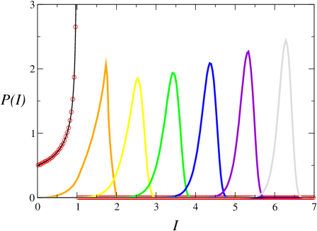
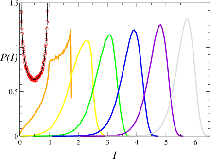
Figure 1: (Color online) Distribution of interference in the CUE ensemble (left) and HOE ensemble (right) for $N=2$ to $N=8$ in steps of 1 (curves from left to right). The full lines for $N=2$ represent the analytical results, eqs.(3) and (8).

III Random circuit ensembles

Shor’s algorithm was recently shown to lead to CUE level statistics Maity and Lakshminarayan , whereas the quantum Fourier transform alone has a regular spectrum (it is a fourth root of the identity matrix), and so does Grover’s algorithm, which is to good approximation a sixth root of the identity matrix Braun (2002). It is therefore natural to ask to what extent are the CUE and the HOE ensembles representative of realistic quantum algorithms?

To answer the above question, we introduce two random quantum circuit ensembles, the random unitary circuit ensemble (UCE), and the random orthogonal circuit ensemble (OCE), constructed to resemble realistic quantum algorithms with $n_{g}$ randomly chosen gates as follows:

• For quantum gate number $i$ ($1\leq i\leq n_{g}$), decide whether to apply a one–qubit gate (with probability $p$) or a multi–qubit gate (with probability $1-p$).

• If gate $i$ is a one–qubit gate, chose randomly, uniformly over all qubits, and independently from all other gates the qubit on which the gate is to act, and pick as gate a random unitary $2\times 2$ matrix from CUE for the construction of an UCE algorithm, or the Hadamard gate for building an OCE algorithm.

• If gate $i$ is a multi–qubit gate, chose randomly, uniformly over all qubits, and independently from all other gates a control qubit (two control qubits) and a target qubit, and apply the CNOT gate (the Toffoli gate) to these qubits for UCE (OCE), respectively.

• Repeat this procedure for all gates $i=1,\ldots,n_{g}$ and concatenate the obtained gates to form the entire quantum algorithm.

A similar ensemble of random quantum circuits was introduced in Emerson et al. (2003), where, however, one random constant depth gate was iterated, and the entangling gate was constructed from simultaneous nearest neighbor interactions. Nevertheless, according to Emerson et al. , one might expect at least an exponential convergence to CUE (HOE) also for UCE (OCE), respectively, and this is what we are going to show numerically.

We first examine the convergence by comparing the distribution $P(s)$ of nearest neighbor spacings $s$ of the eigenphases $\varphi_{l}$ of the $N\times N$ unitary matrices. For large $N$, and average $s$ normalized to unity, CUE leads to a $P(s)$ well approximated by the Wigner surmise Mehta (1991)

$$P_{W}(s)=\frac{32s^{2}}{\pi^{2}}{\rm e}^{-4s^{2}/\pi}\,.$$ (12)

Deviations are of order $10^{-3}$ Haake (1991). For $n=4$, the minimum number of gates that leads to an approximately constant density of eigenphases, such that unfolding the spectrum Mehta (1991) is unnecessary, is $n_{g}\simeq 10$. For even smaller numbers of gates strong peaks at $\varphi=0$ and $\varphi=\pi$ arise in the density of states corresponding to a predominance of real eigenvalues, but otherwise the density is already flat. Fig. 2 shows $P(s)$ for UCE for $n=4$ and several values of $n_{g}$ ($n_{r}=10^{5}$ realizations). For small $n_{g}$, $P(s)$ has a strong peak at $s=0$. The rest of the distribution is between the Poisson result of uncorrelated phases, $P(s)=\exp(-s)$, and the Wigner surmise $P_{W}(s)$. The peak at $s=0$ becomes smaller and smaller as the number of gates increases, and at the same time a more and more pronounced maximum at $s=1$ arises, resulting in a distribution which rapidly approaches the Wigner surmise, eq. (12). For $n_{g}=40$, $P(s)$ is virtually indistinguishable from $P_{W}(s)$. We examine the convergence quantitatively with the help of the quantity

$$F_{s}=\int_{0}^{\infty}\left(\sqrt{P_{UCE}(s)}-\sqrt{P_{W}(s)}\right)^{2}\,ds=2\left(1-\int_{0}^{\infty}\sqrt{P(s)P_{W}(s)}\,ds\right)$$ (13)

which measures a squared distance between the (square roots of) the level spacing distributions $P_{UCE}(s)$ of UCE and $P_{W}(s)$. Fig. 3 shows $F_{s}$ as function of $n_{g}$ for UCE for various values of $p$ and $n=4$ qubits, obtained from $10^{3}$ random algorithms. For $p$ different from 0 and 1, $F_{s}$ decays to a good approximation exponentially as $\sim\exp(-b(n,p)n_{g})$, with a rate $b$ that depends on $p$ and $n$, before saturating at a small level largely independent of $p$. The latter is due to the numerical fluctuations in $P(s)$ present for any finite $N$, as is easily checked by varying $N$. The finite precision of $P_{W}(s)$ for $N>2$ sets another lower bound on the values of $F$ that can be possible achieved. Fig. 3 also shows that $b(n,p)$, as obtained from a fit of $\ln F_{s}$ to a linear function of $n_{g}$ between $F_{2}=2$ and $F_{2}=0.1$ has a maximum around $p=0.5$. The convergence rates decrease with increasing $n$, and the maximum of the convergence rate as function of $p$ shifts to somewhat smaller values of $p$.

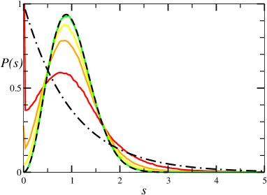
Figure 2: (Color online) $P(s)$ for $n_{g}=10$ (red), 15 (orange) 20 (yellow) and 40 (green — increasing values of $P(1)$ in this order) for UCE with $n=4$ and $p=0.5$, $n_{r}=10^{5}$ matrices, compared to the Wigner surmise $P_{W}(s)$ (dashed black line) and the Poisson result, $P(s)=\exp(-s)$ (dashed-dotted black line).

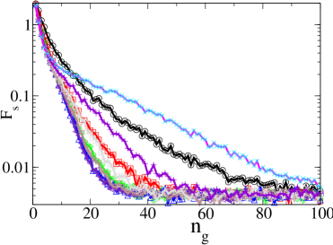
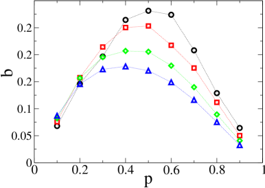
Figure 3: (Color online) Convergence of $P(s)$ for UCE to $P_{W}(s)$ as function of $n_{g}$ for $n=4$ qubits, $n_{r}=10^{3}$, and different values of $p$: $p=0.1$ black squares, $p=0.2$ red squares, $p=0.3$ green diamonds, $p=0.4$ blue triangles up, $p=0.5$ indigo triangles left, $p=0.6$ brown triangles down, $p=0.7$ grey triangles right, $p=0.8$ violet pluses, and $p=0.9$ magenta Xs (left). Rate of convergence $b$ as function of the probability $p$ for $n=3$ (circles), $n=4$ (squares), $n=5$ (diamonds), and $n=6$ (triangles up).

Numerical evidence presented in Pozniak et al. (1998) indicates the same form of $P(s)$ for HOE as for CUE, eq.(12), in particular a quadratic level repulsion $P(s)\propto s^{2}$ for $s\ll 1$. We have examined the convergence of OCE to HOE based on $P(s)\to P_{W}(s)$ as well, and have found similar results as in Fig.3. However, it is clearly not possible to determine the limiting ensemble based on $P(s)$ alone. We therefore also examined directly the interference distributions $P({\cal I})$ for both random circuit ensembles, as $P({\cal I})$ is, after all, what we are interested in.

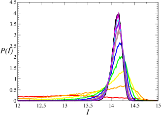
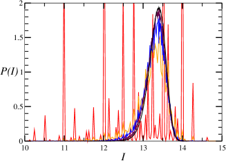
Figure 4: (Color online) Interference distribution $P_{UCE,N}({\cal I})$ (left), for $n_{g}=10,20,30,40,50,60,70,80,90,100$, maxima increasing in this order, and $P_{OCE,N}$ (right) for $n_{g}=20,50,70,100$ (red, orange, blue, maroon, respectively) compared to the $P({\cal I})$ of the circular random matrix ensembles (black lines). All curves have $n=4$ ($N=16$); $n_{r}=10^{5}$ random realizations were used for UCE and OCE, $n_{r}=10^{7}$ for CUE and HOE.

Fig.4 shows how the interference distribution of UCE for $n=4$ evolves between $n_{g}=10$ to $n_{g}=100$ from a broad flat distribution to the strongly peaked interference distribution of CUE. The interference distribution $P_{OCE,N}({\cal I})$ for OCE fluctuates much more for a given number of gates compared to the one for UCE, $P_{UCE,N}({\cal I})$, but rapidly approaches $P_{HOE,N}(I)$ as well. To examine the convergence quantitatively, we define the quantity $F_{I}$ as in (13), but with $P(s)$ and $P_{W}(s)$ replaced by the interference distributions $P_{UCE,N}({\cal I})$ and $P_{CUE,N}({\cal I})$ for UCE and CUE (by $P_{OCE,N}({\cal I})$ and $P_{HOE,N}({\cal I})$ for OCE and HOE). Note that $P_{\rm CUE}({\cal I})$ and $P_{\rm HOE}({\cal I})$ have now to be computed numerically as well. We did so for the same dimension of Hilbert space $N=2^{n}$ considered for UCE and OCE. We used $n_{r}=10^{7}$ realizations for $n\in\{4,5\}$, for both CUE and HOE, as well as for $n=6$, HOE; $n_{r}=5\cdot 10^{6}$ for $n=7$, and $n_{r}=10^{6}$ for $n=8$ (HOE); and $n_{r}=4\cdot 10^{5}$ for $n=6$ (CUE). The number of realizations chosen for the OCE and UCE ensembles was $10^{5}$, with the exception of $n_{r}=4\cdot 10^{5}$ for $n=6$, UCE. Fig.5 shows the results for $F_{I}(n_{g})$ for $n=5$. The curves for the other values of $n$ examined ($n\in\{4,6,7,8\}$) look very similar, but the convergence slows down with increasing $n$.

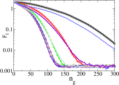
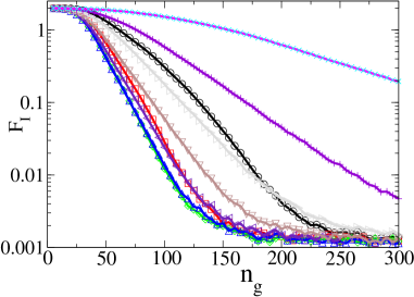
Figure 5: (Color online) Convergence of $P({\cal I})$ for UCE (left) and OCE (right) to the interference distribution of CUE and HOE, respectively, as function of $n_{g}$ for $n=5$ qubits ($N=32$) and different values of $p$. Same symbols as in Fig.3.

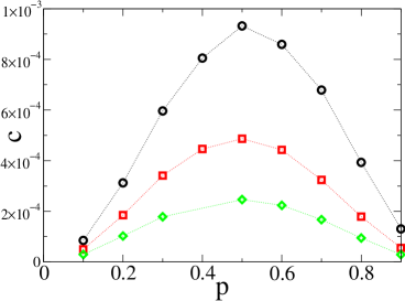
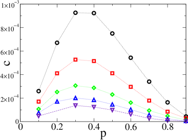
Figure 6: (Color online) Dependence of the fitted Gaussian convergence rate $c$ on the probability $p$ for a single qubit gate (a random $U(2)$ for UCE (left) and Hadamard for OCE (right)) for various numbers of qubits (circles, squares, diamonds for $n=4,5,6$), respectively, and in addition triangles up and triangles down for $n=7,8$ for UCE.

$F_{I}(n_{g})$ for both UCE and OCE is very well fitted by a Gaussian, at least up to the point where the crossover to the saturated behavior occurs. This is in contrast to the exponential convergence of $P(s)$. A fit of $\ln F_{I}(n_{g})$ to $a-c(n,p)\,n_{g}^{2}$ in the range $2\geq F_{I}(n_{g})\geq 0.01$ yields $c\sim 10^{-4}$ for $4\leq n\leq 6$, with a maximum of $c$ around $p\sim 0.5$ for both OCE and UCE (see Fig.6).

The exponential (or even Gaussian) convergence of the random circuit ensembles to the corresponding circular ensembles as function of the number of quantum gates provides a new way of economically creating random unitary operators with a flat distribution with respect to the appropriate Haar measure in an exponentially large Hilbert space. The method will work on any quantum computer on which the relevant universal set of gates is available. The OCE is particularly interesting, as the only randomness resides in the indices of the qubits selected as entry of the Hadamard or Toffoli gates. About $2n_{g}$ such random numbers $i$ in the range $0\leq i\leq n-1$ are needed for $p=1/2$. This offers the possibility to construct truly random operators, with only a logarithmic overhead of qubits: A small register of $n_{a}\sim 3\log_{2}n+1$ auxiliary qubits can be brought repeatedly into superposition of all computational states by applying a Hadamard gate to each qubit; then the register is measured in the computational basis and gives a random number. The outcome of one particular qubit (the highest significant, say), can be used to choose between the Hadamard and Toffoli gates, and the remaining bits specify the qubit(s) on which to act. Obviously, one might as well use the actual work qubits to generate these random numbers initially and store them for later use in the quantum algorithm.

The question remains open whether the method presented here is efficient in the sense that the number of quantum gates $n_{g}$ needed for a given fidelity $F_{I}$ or $F_{s}$ increases at most polynomially with $n$. This would require that the exponents $c(n,p)$ and $b(n,p)$ decay no faster than an inverse power of $n$ for a given $p$. The same problem was encountered in Emerson et al. (2003, ) and so far no definite answer has been found. In order to address the question numerically, much larger values of $n$ have to be considered. The study of the interference distributions is clearly not well suited for this purpose, as each algorithm (i.e. a very large dimensional matrix) gives only one number.

IV Summary

As a summary, we have introduced two ensembles of random quantum algorithms, UCE for general unitary algorithms, and OCE for real orthogonal algorithms. We have provided numerical evidence that these ensembles converge for sufficiently large numbers of gates and for a finite probability for both one–qubit and two–qubit gates (or three-qubit gates), to the well–known random matrix ensembles CUE and HOE, respectively, at least in the sense of coinciding level spacing distributions and interference distributions. One might consider these ensembles therefore as a new way of efficiently creating random unitaries from the corresponding Haar measure Emerson et al. (2003, ). The method is universal in the sense that it runs on any quantum computer with a universal set of quantum gates. We have calculated numerical distributions of interference over the CUE and HOE ensembles, and have provided exact analytical formulas for the lowest moments. For large Hilbert space dimensions $N$, the interference distributions over CUE and HOE are peaked on their average values $\langle{\cal I}\rangle_{U,N}\simeq N-2$ and $\langle{\cal I}\rangle_{O.N}\simeq N-3$, respectively, with a width that decays $\propto 1/N$ in both cases. Thus, randomly picked unitary quantum algorithms contain with high probability basically the same exponentially large amount of interference ${\cal I}\sim N$. This result is reminiscent of similar findings for the amount of entanglement in a random quantum state Cappellini et al. . Grover’s search algorithm is therefore remarkably exceptional in the sense that its non–generic part (i.e. the part after bringing the computer into a superposition of all computational states) uses only a small amount of interference (the whole algorithm including the initial Hadamard gates produces exponential interference Braun and Georgeot (2006)).

Acknowledgments: We would like to thank Bertrand Georgeot for interesting discussions, and CALMIP (Toulouse) for the use of their computers. This work was supported by the Agence National de la Recherche (ANR), project INFOSYSQQ, and the EC IST-FET project EDIQIP.

References

- Bennett and DiVincenzo (2000) C. H. Bennett and D. P. DiVincenzo, Nature 404, 247 (2000).
- Curty et al. (2004) M. Curty, M. Lewenstein, and N. Lütkenhaus, Phys. Rev. Lett. 92, 217903 (2004).
- Bennett et al. (1993) C. H. Bennett, G. Brassard, C. Crepeau, R. Jozsa, A. Peres, and W. Wootters, Phys. Rev. Lett. 70, 1895 (1993).
- Lewenstein et al. (2000) M. Lewenstein, D. Bruss, J. I. Cirac, B. Kraus, M. Kus, J. Samsonowicz, A. Sanpera, and R. Tarrach, J. Mod. Optics 47, 2841 (2000).
- Jozsa and Linden (2003) R. Jozsa and N. Linden, Proc. R. Soc. Lond. A 459, 2011 (2003).
- Ramsey (1960) N. Ramsey, Phys. Rev. 78, 695 (1960).
- Brune et al. (1996) M. Brune, E. Hagley, J. Dreyer, X. Maître, A. Maali, C. Wunderlich, J. M. Raimond, and S. Haroche, Phys. Rev. Lett. 77, 4887 (1996).
- Vion et al. (2002) D. Vion, A. Aassime, A. Cottet, P. Joyez, H. Pothier, C. Urbina, D. Esteve, and M. Devoret, Science 296, 886 (2002).
- Cabrillo et al. (1999) C. Cabrillo, J. I. Cirac, P. García-Fernández, and P. Zoller, Phys. Rev. A 59, 1025 (1999).
- Beaudry et al. (2005) M. Beaudry, J. M. Fernandez, and M. Holzer, Theor. Comp. Science 345, 206 (2005).
- Braun and Georgeot (2006) D. Braun and B. Georgeot, Phys. Rev. A 73, 022314 (2006).
- Shor (1994) P. W. Shor (IEEE Computer Society, Los Alamitos, CA, 1994).
- Grover (1997) L. K. Grover, Phys. Rev. Lett. 79, 325 (1997).
- DiVincenzo (1995) D. P. DiVincenzo, 1995 51, 1015 (1995).
- Barenco (1995) A. Barenco, Proc. R. Soc. Lond. A 51, 1015 (1995).
- Sleator and Weinfurter (1995) T. Sleator and H. Weinfurter, Phys. Rev. Lett. 74, 4087 (1995).
- (17) Y. Shi, eprint quant-ph/0205115.
- (18) D. Aharonov, eprint quant-ph/0301040.
- Pozniak et al. (1998) M. Pozniak, K. Życzkowski, and M. Kus, J. Phys. A 31, 1059 (1998).
- Hurwitz (1897) A. Hurwitz, Nachr. Ges. Wiss. Gött. Math.-Phys. Kl. 71 71 (1897).
- Aubert and Lam (2003) S. Aubert and C. Lam, J.Math.Phys. 44, 6112 (2003).
- Mehta (1991) M. L. Mehta, Random Matrices (Academic Press, New York, 1991), 2nd ed.
- Braun (2006) D. Braun, to be published (2006).
- (24) K. Maity and A. Lakshminarayan, eprint quant-ph/0604111.
- Braun (2002) D. Braun, Phys. Rev. A 65, 042317 (2002).
- Emerson et al. (2003) J. Emerson, Y. Weinstein, M. Saraceno, S. Lloyd, and d. Cory, Science 302, 2098 (2003).
- (27) J. Emerson, E. Livine, and S. Lloyd, eprint quant-ph/0503210.
- Haake (1991) F. Haake, Quantum Signatures of Chaos (Springer, Berlin, 1991).
- (29) V. Cappellini, H.-J. Sommers, and K. Życzkowski, eprint quant-ph/0605251.