Non-Abelian Generalization of Off-Diagonal Geometric Phases

Abstract

If a quantum system evolves in a noncyclic fashion the corresponding geometric phase or holonomy may not be fully defined. Off-diagonal geometric phases have been developed to deal with such cases. Here, we generalize these phases to the non-Abelian case, by introducing off-diagonal holonomies that involve evolution of more than one subspace of the underlying Hilbert space. Physical realizations of the off-diagonal holonomies in adiabatic evolution and interferometry are put forward.

I Introduction

A quantal system that fails to return to its initial state after some prescribed elapse of time may acquire a well-defined geometric phase samuel88 . An interesting feature of this noncyclic geometric phase is that it becomes undefined when the initial and final states are orthogonal. This gives rise to a nodal point structure that can be monitored experimentally in a history-dependent manner bhandari91 ; bhandari92a ; bhandari92b ; bhandari93 . In the hope to recover some of the lost interference information at the nodal points of the noncyclic geometric phase, Manini and Pistolesi manini00 introduced off-diagonal geometric phases for adiabatic evolutions of pure states. These quantities may be defined in cases where the standard geometric phase is not. The adiabatic requirement on the evolution in ref. manini00 was lifted by Mukunda et. al. mukunda02 , and Hasegawa et. al. hasegawa01 ; hasegawa02 provided an experimental verification of the second order off-diagonal geometric phase for neutron spin. Theories for off-diagonal phases and holonomies for mixed quantal states have been developed filipp03a ; filipp03b ; tong05 ; filipp05 .

Wilczek and Zee wilczek84 showed that the geometric phase factor generalizes to a unitary state change, often referred to as a non-Abelian quantum holonomy, when considering cyclic adiabatic evolution governed by a degenerate Hamiltonian. The relevance of non-Abelian holonomies for universal fault tolerant quantum computation has been demonstrated in refs. zanardi99 ; pachos00a ; pachos00b ; duan01 ; recati02 ; faoro03 . The non-Abelian quantum holonomies have been generalized to nonadiabatic anandan88 , discrete sjoqvist06 , and noncyclic evolutions mostafazadeh99 ; kult06 . As for the geometric phase, the holonomy may be undefined when the evolution is noncyclic. In the non-Abelian case we also have the additional possibility that the holonomy is partially defined kult06 .

In this Letter, we extend ref. manini00 and introduce non-Abelian off-diagonal holonomies. We demonstrate that the off-diagonal holonomies retain holonomy information when the standard noncyclic ones mostafazadeh99 ; kult06 are undefined. We also suggest physical realizations of the off-diagonal holonomies using interferometry, both in adiabatic and nonadiabatic settings.

II Off-diagonal Holonomies

Consider a smoothly parameterized decomposition

$$\mathcal{H}=\mathcal{H}_{1}(s)\oplus\cdots\oplus\mathcal{H}_{\eta}(s),\ s\in[0,1],$$ (1)

of an $N$-dimensional Hilbert space $\mathcal{H}$ into $\eta$ mutually orthogonal subspaces. It is to be noted that this parameter-dependent decomposition can arise in different ways, e.g., it may consist of the instantaneous eigenspaces of some $s$-dependent Hamiltonian wilczek84 , or of some arbitrary decomposition that evolves under the Schrödinger equation anandan88 . Assume that $\dim[\mathcal{H}_{l}(s)]=n_{l}$, $\forall s\in[0,1]$, and $l=1,\ldots,\eta$. Thus, each family $\mathcal{H}_{l}(s)$ of subspaces defines a curve $\mathcal{C}_{l}$ in the Grassmann manifold $\mathcal{G}(N;n_{l})$, i.e., the set of $n_{l}$-dimensional subspaces in the $N$-dimensional Hilbert space greub73 . For each such curve, we introduce the quantities

$$\Gamma_{l}=\lim_{\delta s\rightarrow 0}P_{l}(1)P_{l}(1-\delta s)\cdots P_{l}(\delta s)P_{l}(0),$$ (2)

where $P_{l}(s)$ is the projection operator onto the subspace $\mathcal{H}_{l}(s)$. This definition makes $\Gamma_{l}$ explicitly gauge invariant. Note also that the limit $\delta s\rightarrow 0$ in Eq. (2) makes $\Gamma_{l}$ uniquely determined for any sufficiently smooth curve $\mathcal{C}_{l}$ in the Grassman manifold. We furthermore define

$$\sigma_{kl}=P_{k}(0)\Gamma_{l}.$$ (3)

Let $\{|k^{i}(s)\rangle\}_{i=1}^{n_{k}}$ and $\{|l^{i}(s)\rangle\}_{i=1}^{n_{l}}$ be orthonormal bases for subspaces $\mathcal{H}_{k}(s)$ and $\mathcal{H}_{l}(s)$, respectively, in terms of which

$$\sigma_{kl} = \sum_{ij}[(\mathcal{F}^{k}_{0}|\mathcal{F}^{l}_{1}){\bf P}e^{\int_{0}^{1}\boldsymbol{A}_{l}(s)ds}]_{ij}|k^{i}(0)\rangle\langle l^{j}(0)|$$ (4)

$$= \sum_{ij}[\boldsymbol{\sigma}^{kl}]_{ij}|k^{i}(0)\rangle\langle l^{j}(0)|.$$

Here, $(\mathcal{F}^{k}_{0}|\mathcal{F}^{l}_{1})$ is a $n_{k}\times n_{l}$ matrix with components $(\mathcal{F}^{k}_{0}|\mathcal{F}^{l}_{1})_{ij}=\langle k^{i}(0)|l^{j}(1)\rangle$ and $[\boldsymbol{A}_{l}(s)]_{ij}=\langle\partial_{s}l^{i}(s)|l^{j}(s)\rangle$ is the Wilczek-Zee connection along $\mathcal{C}_{l}$ in $\mathcal{G}(N;n_{l})$.

The unitary part $\Phi[\boldsymbol{\sigma}^{ll}]$ is the holonomy in ref. kult06 associated with the (open) path $\mathcal{C}_{l}$. It seems natural to ask whether we can interpret the matrices $\boldsymbol{\sigma}^{kl},\ k\neq l,$ in a similar fashion. To answer this, we need to see how these matrices behave under a gauge transformation, i.e., a change of frames $|l^{i}(s)\rangle\rightarrow|\widetilde{l}^{i}(s)\rangle=\sum_{j}|l^{j}(s)\rangle[\boldsymbol{U}_{l}(s)]_{ji}$, where $\{\boldsymbol{U}_{l}(s)\}_{l=1}^{\eta}$ are unitary matrices. Under such a transformation the matrices ${\bf P}e^{\int_{0}^{1}\boldsymbol{A}_{l}(s)ds}$ and $(\mathcal{F}^{k}_{0}|\mathcal{F}^{l}_{1})$ undergo the following changes

$${\bf P}e^{\int_{0}^{1}\boldsymbol{A}_{l}(s)ds} \rightarrow \boldsymbol{U}_{l}^{\dagger}(1){\bf P}e^{\int_{0}^{1}\boldsymbol{A}_{l}(s)ds}\boldsymbol{U}_{l}(0),$$

$$(\mathcal{F}^{k}_{0}|\mathcal{F}^{l}_{1}) \rightarrow \boldsymbol{U}_{k}^{\dagger}(0)(\mathcal{F}^{k}_{0}|\mathcal{F}^{l}_{1})\boldsymbol{U}_{l}(1).$$ (5)

Consequently, $\boldsymbol{\sigma}^{kl}$ transforms as

$$\boldsymbol{\sigma}^{kl}\rightarrow\boldsymbol{U}_{k}^{\dagger}(0)\boldsymbol{\sigma}^{kl}\boldsymbol{U}_{l}(0),$$ (6)

i.e., noncovariantly unless $k=l$. Thus, the matrices $\boldsymbol{\sigma}^{kl}$, $k\neq l$, fail to reflect the geometry of the paths $\mathcal{C}_{k}$ and $\mathcal{C}_{l}$. However, the specific behavior of $\boldsymbol{\sigma}^{kl}$ under gauge transformations suggests that we consider the operator

$$\gamma_{l_{1}\ldots l_{\kappa}} = \sigma_{l_{1}l_{\kappa}}\sigma_{l_{\kappa}l_{\kappa-1}}\cdots\sigma_{l_{3}l_{2}}\sigma_{l_{2}l_{1}}$$ (7)

$$= \sum_{ij}[\boldsymbol{\gamma}^{l_{1}\ldots l_{\kappa}}]_{ij}|l_{1}^{i}(0)\rangle\langle l_{1}^{j}(0)|,$$

where $\boldsymbol{\gamma}^{l_{1}\ldots l_{\kappa}}$ is the matrix

$$\boldsymbol{\gamma}^{l_{1}\ldots l_{\kappa}}=\boldsymbol{\sigma}^{l_{1}l_{\kappa}}\boldsymbol{\sigma}^{l_{\kappa}l_{\kappa-1}}\cdots\boldsymbol{\sigma}^{l_{3}l_{2}}\boldsymbol{\sigma}^{l_{2}l_{1}}.$$ (8)

We can use these operators and matrices to define gauge covariant quantities, since $\Phi\big{[}\boldsymbol{\gamma}^{l_{1}\ldots l_{\kappa}}\big{]}\rightarrow\boldsymbol{U}_{l_{1}}^{\dagger}(0)\Phi\big{[}\boldsymbol{\gamma}^{l_{1}l_{2}\ldots l_{\kappa}}\big{]}\boldsymbol{U}_{l_{1}}(0)$ from eq. (6). Thus, we propose to take

$$\boldsymbol{U}_{g}^{(\kappa)}[\mathcal{C}_{l_{1}},\ldots,\mathcal{C}_{l_{\kappa}}]=\Phi\big{[}\boldsymbol{\gamma}^{l_{1}\ldots l_{\kappa}}\big{]}$$ (9)

as the gauge covariant non-Abelian holonomies of order $\kappa$, and thus generalizing the approach of ref. manini00 to the non-Abelian case. We extend the range of $\kappa$ by defining $\boldsymbol{U}_{g}^{(1)}[\mathcal{C}_{l}]=\Phi\big{[}\boldsymbol{\sigma}^{ll}\big{]}$, i.e., the first order ($\kappa=1$) holonomies are taken to be the open path holonomies in refs. mostafazadeh99 ; kult06 .

Note that the definition in eq. (9) allows any sequence $(l_{1},\ldots,l_{\kappa})$. This includes cases like, e.g., $\boldsymbol{\gamma}^{111}$, which cannot be regarded as an “off-diagonal” object. Hence, eq. (9) can be regarded as a general definition of holonomies of degree $\kappa$, both diagonal and off-diagonal. To define genuinely off-diagonal holonomies we obtain a reasonable subclass if we require that $(l_{1},\ldots,l_{\kappa})$ contains each number at most once. We let $\mathbb{I}_{\kappa}^{\eta}$ denote all vectors $(l_{1},\ldots,l_{\kappa})$ with $l_{j}\in\{1,\ldots,\eta\}$, such that none of the numbers occurs twice, e.g., $(2,5,3)\in\mathbb{I}_{3}^{6}$ but $(6,4,6,2)\notin\mathbb{I}_{4}^{6}$. We refer to the set of holonomies $\boldsymbol{U}_{g}^{(\kappa)}[\mathcal{C}_{l_{1}},\ldots,\mathcal{C}_{l_{\kappa}}]$ with $(l_{1},\ldots,l_{\kappa})\in\mathbb{I}_{\kappa}^{\eta}$ with $2\leq\kappa\leq\eta$, as “strictly off-diagonal holonomies”.

For a cyclic evolution, characterized by $\mathcal{H}_{l}(1)=\mathcal{H}_{l}(0),\ l=1,\ldots,\eta$, the standard holonomies $\boldsymbol{U}_{g}^{(1)}[\mathcal{C}_{l}]$ are fully defined. On the other hand, in this case we have $\boldsymbol{\gamma}^{l_{1}\ldots l_{\kappa}}=0$, $(l_{1},\ldots,l_{\kappa})\in\mathbb{I}^{\eta}_{\kappa}$, $\kappa\geq 2$, which implies that all strictly off-diagonal holonomies are undefined for cyclic evolution. Thus, just as in the Abelian case manini00 , the standard holonomies contain all nontrivial information about $\mathcal{C}_{1},\ldots,\mathcal{C}_{\eta}$ when these are loops.

In the case where $n_{l}=1$, $l=1,\ldots,\eta$, the matrices $(\mathcal{F}^{k}_{0}|\mathcal{F}^{l}_{1})$ and ${\bf P}e^{\int_{0}^{1}\boldsymbol{A}_{l}(s)ds}$ reduce to the complex numbers $\langle k(0)|l(1)\rangle$ and $e^{-\int_{0}^{1}\langle l(s)|\partial_{s}l(s)\rangle ds}$, respectively. This leads to the off-diagonal geometric phase factors

$$\boldsymbol{U}_{g}^{(\kappa)}[\mathcal{C}_{l_{1}},\ldots,\mathcal{C}_{l_{\kappa}}]=\Phi\big{[}\langle l_{1}(0)|l_{\kappa}(1)\rangle$$

$$\times e^{-\int_{0}^{1}\langle l_{\kappa}(s)|\partial_{s}l_{\kappa}(s)\rangle ds}\cdots\langle l_{2}(0)|l_{1}(1)\rangle$$

$$\times e^{-\int_{0}^{1}\langle l_{1}(s)|\partial_{s}l_{1}(s)\rangle ds}\big{]},$$ (10)

which coincide with $\Phi\big{[}\gamma^{(\kappa)\Gamma}_{l_{1}l_{\kappa}l_{\kappa-1}\ldots l_{2}}\big{]}$ in ref. manini00 .

Manini and Pistolesi manini00 suggest an interpretation of their off-diagonal geometric phases in terms of Berry phases for single closed paths. In the second order case, these paths consist of the segments $\mathcal{C}_{k}$, $\mathcal{C}_{l}$, $G_{kl}$, and $G_{lk}$, where $G_{kl}$ geodesically connects the final point of $\mathcal{C}_{k}$ with the starting point of $\mathcal{C}_{l}$, and vice versa for $G_{lk}$ (see fig. 1 of ref. manini00 ). In the general non-Abelian case, however, this interpretation is difficult to maintain. Apart from the special case when $n_{1}=n_{2}=\ldots=n_{\kappa}$, it is not possible to join the curves $\mathcal{C}_{l_{1}},\ldots,\mathcal{C}_{l_{\kappa}}$, due to the mismatch of dimensions, and thus the closure using geodesics is not applicable. This observation shows that the off-diagonal holonomies in general cannot be interpreted as standard Wilczek-Zee quantum holonomies for closed paths wilczek84 , and that the off-diagonal holonomies therefore are genuinely new concepts associated with the evolution of quantum systems. Another consequence of the fact that we can have different $n_{l}$ is that the rank of $\boldsymbol{\gamma}^{l_{1}\ldots l_{\kappa}}$ cannot be larger than the smallest $n_{l}$ (see 2.17.8 of ref. marcus64 ), and thus may be less than $n_{l_{1}}$.

The non-Abelian character of the off-diagonal holonomies $\boldsymbol{U}^{(\kappa)}[\mathcal{C}_{1},\ldots,\mathcal{C}_{\kappa}]$ implies that they are not invariant under cyclic permutations of the indexes $(l_{1},\ldots,l_{\kappa})$. It may even be the case that two off-diagonal holonomies that differ only by a cyclic permutation have different rank, since the smallest $n_{l}$ only provides an upper bound for the rank of $\boldsymbol{\gamma}^{l_{1}\ldots l_{\kappa}}$. Furthermore, as is exemplified below it is also possible that $\boldsymbol{\gamma}^{l_{1}\ldots l_{\kappa}}$ may have path-dependent nodal points if $\kappa\geq 2$.

III Where did the phase information go?

As noted above, all strictly off-diagonal holonomies are undefined for cyclic evolutions, in analogy with the standard cyclic off-diagonal geometric phases. Conversely, the noncyclic geometric phases are undefined when the states at the initial and final points of the curves are orthogonal, i.e., there exist nodal points where these phases are undefined. The hope to recover this lost phase information appears to have been one of the primary reasons for Manini and Pistolesi to introduce off-diagonal geometric phases. However, the issue concerning the possible recovery of phase information was never explicitly investigated in ref. manini00 . In the following we elucidate some aspects of this question in the case of non-Abelian off-diagonal holonomies.

Let us first analyze what happens if the rank of some of the overlap matrices $(\mathcal{F}_{0}^{l}|\mathcal{F}_{1}^{l})$ is greater than zero but less than their subspace dimension $n_{l}$. This is a situation where the corresponding holonomies become partial kult06 ; a phenomenon that has no counterpart in the Abelian case. To aid us in this analysis we introduce the unitary $N\times N$ matrix

$$\boldsymbol{S}_{\textrm{tot}}=\begin{pmatrix}\boldsymbol{\sigma}^{11}&\ldots&\boldsymbol{\sigma}^{1\eta}\\ \vdots&\ddots&\vdots\\ \boldsymbol{\sigma}^{\eta 1}&\ldots&\boldsymbol{\sigma}^{\eta\eta}\end{pmatrix}.$$ (11)

It follows from unitarity that $R(\boldsymbol{S}_{\textrm{tot}})=N$, where $R(\boldsymbol{X})$ denotes the rank of matrix $\boldsymbol{X}$. Furthermore, for every $l=1,\ldots,\eta$, it holds that $\sum_{k}\boldsymbol{\sigma}^{kl\dagger}\boldsymbol{\sigma}^{kl}=\sum_{k}\boldsymbol{\sigma}^{lk}\boldsymbol{\sigma}^{lk\dagger}=\boldsymbol{1}_{n_{l}\times n_{l}}$, where $\boldsymbol{1}_{n_{l}\times n_{l}}$ denotes the $n_{l}\times n_{l}$ identity matrix. This entails that (see 2.17.2 and 2.17.5 of ref. marcus64 ) $\sum_{k}R(\boldsymbol{\sigma}^{kl})\geq n_{l}$ and $\sum_{k}R(\boldsymbol{\sigma}^{lk})\geq n_{l}$. So, if $R(\boldsymbol{\sigma}^{ll})=n_{l}-n$, then $\sum_{k\neq l}R(\boldsymbol{\sigma}^{kl})\geq n$ and $\sum_{k\neq l}R(\boldsymbol{\sigma}^{lk})\geq n$. In other words, when the overlap matrix $(\mathcal{F}_{0}^{l}|\mathcal{F}_{1}^{l})$ decreases by $n$ in rank, the lower bound for the sum of the ranks of the matrices $\boldsymbol{\sigma}^{kl}$ increases by the same amount. Thus, the “holonomy information” that is lost when the holonomy of the curve $\mathcal{C}_{l}$ becomes partial is transferred to the matrices $\boldsymbol{\sigma}^{kl}$.

A perhaps more significant question is whether the rank of the matrices $\boldsymbol{\gamma}^{l_{1}\ldots l_{\kappa}}$ depends on the rank of the overlap matrix $(\mathcal{F}_{0}^{l}|\mathcal{F}_{1}^{l})$ in a manner similar to what was discussed above for the matrices $\boldsymbol{\sigma}^{kl}$. One can demonstrate with a simple counterexample that no such relation exists. Assume $\eta=3$ and $n_{1}=n_{2}=n_{3}=2$. Furthermore, assume that $\boldsymbol{\sigma}^{13}$, $\boldsymbol{\sigma}^{21}$, and $\boldsymbol{\sigma}^{32}$ are the $2\times 2$ zero matrix, and

$${\boldsymbol{\sigma}^{11}}^{\dagger}={\boldsymbol{\sigma}^{22}}^{\dagger}={\boldsymbol{\sigma}^{33}}^{\dagger}=\boldsymbol{\sigma}^{12}=\boldsymbol{\sigma}^{23}=\boldsymbol{\sigma}^{31}=\begin{pmatrix}0&0\\ 1&0\end{pmatrix}.$$

One may verify that the corresponding matrix $\boldsymbol{S}_{\textrm{tot}}$ is unitary. In this example $\boldsymbol{\gamma}^{kl}=0,\ \forall k,l$, and $\boldsymbol{\gamma}^{klm}=0,\ \forall k,l,m$. Hence, although none of the overlap matrices $(\mathcal{F}^{l}_{0}|\mathcal{F}^{l}_{1})$ are of full rank, all strictly off-diagonal holonomies vanish, even those of higher order.

Finally, we ask what happens if the matrices $\boldsymbol{\sigma}^{ll}$ are zero for all $l=1,\ldots,\eta$. We prove by reductio ad absurdum that at least one of the strictly off-diagonal holonomies must have nonzero rank. Assume $\boldsymbol{\sigma}^{ll}=0$, for $l=1,\ldots,\eta$, and $\boldsymbol{\gamma}^{l_{1}\ldots l_{\kappa}}=0$, for $(l_{1},\ldots,l_{\kappa})\in\mathbb{I}_{\kappa}^{\eta}$, $\kappa\geq 2$. Consider an arbitrary string $(l_{1},\ldots,l_{\nu})$ consisting of the integers $1$ to $\eta$, and with $\nu\geq 2$. If $(l_{1},\ldots,l_{\nu})\in\mathbb{I}_{\nu}^{\eta}$ ($\nu\leq\eta$), then by assumption $\boldsymbol{\gamma}^{l_{1}\ldots l_{\nu}}=0$. If $(l_{1},\ldots,l_{\nu})\notin\mathbb{I}_{\nu}^{\eta}$, then take one of the smallest subsequences $(l_{\alpha},l_{\alpha+1},\ldots,l_{\beta-1},l_{\beta})$ that begins and ends with the same number (i.e., $l_{\beta}=l_{\alpha}$). In this subsequence there is no other repetitions (otherwise there exists a smaller subsequence). It follows that $\boldsymbol{\gamma}^{l_{1}\ldots l_{\nu}}=\boldsymbol{\sigma}^{l_{1}l_{\nu}}\cdots\boldsymbol{\sigma}^{l_{\beta+1}l_{\beta}}\boldsymbol{\gamma}^{l_{\alpha}\ldots l_{\beta-1}}\boldsymbol{\sigma}^{l_{\alpha}l_{\alpha-1}}\cdots\boldsymbol{\sigma}^{l_{2}l_{1}}$. Moreover, $(l_{\alpha},\ldots,l_{\beta-1})\in\mathbb{I}^{\eta}_{\beta-\alpha-1}$. If $\beta-\alpha=1$, then $\boldsymbol{\gamma}^{l_{\alpha}\ldots l_{\beta-1}}=\boldsymbol{\sigma}^{l_{\alpha}l_{\alpha}}=0$, otherwise $\boldsymbol{\gamma}^{l_{\alpha}\ldots l_{\beta-1}}=0$ by assumption. We proceed by noting that ${\textrm{Tr}}\left(\boldsymbol{S}_{\textrm{tot}}^{\nu}\right)=\sum_{l_{1}\ldots l_{\nu}}{\textrm{Tr}}\boldsymbol{\gamma}^{l_{1}\ldots l_{\nu}}=0$, for all $\nu=1,2,\ldots$, as a consequence of our assumptions. However, this cannot be the case since $\boldsymbol{S}_{\textrm{tot}}$ is a unitary matrix. Therefore, our assumptions must be wrong, and at least one of the strictly off-diagonal holonomies must have nonzero rank. By the above findings we can conclude that the holonomy information lost in the the nodal points of the non-Abelian noncyclic holonomies indeed can be retained in some sense, but that the structure is much more intricate and rich than in the Abelian case, due to the existence of partial holonomies in the non-Abelian setting.

IV Example

We illustrate the off-diagonal holonomies by an example in the adiabatic context. We let the system evolve under the action of a slowly varying Hamiltonian. Let us consider the tripod system duan01 ; unanyan99 modeled by the parameter-dependent four-state Hamiltonian $H(s)=\omega|e\rangle(\sin\theta(s)\cos\varphi(s)\langle 0|+\sin\theta(s)\sin\varphi(s)\langle 1|+\cos\theta(s)\langle a|)+\textrm{h.c.}$, exhibiting two nondegenerate ‘bright’ states $|\mathcal{F}_{s}^{\pm})=\{|B^{\pm}(s)\rangle\}$ with energy $\pm\omega$ and a doubly degenerate ‘dark’ zero energy eigenspace $|\mathcal{F}_{s}^{d})=\{|D^{1}(s)\rangle,|D^{2}(s)\rangle\}$. Explicitly, we may choose

$$|B^{\pm}\rangle = \frac{1}{\sqrt{2}}\Big{(}|e\rangle\pm\sin\theta\cos\varphi|0\rangle\pm\sin\theta\sin\varphi|1\rangle$$

$$\pm\cos\theta|a\rangle\Big{)},$$

$$|D_{1}\rangle = \cos\theta\cos\varphi|0\rangle+\cos\theta\sin\varphi|1\rangle-\sin\theta|a\rangle,$$

$$|D_{2}\rangle = -\sin\varphi|0\rangle+\cos\varphi|1\rangle.$$ (12)

Consider paths $(0,0)\rightarrow(\theta_{1},\varphi_{1})$ in parameter space $(\theta,\varphi)$. For each such path the energy eigenstates define paths $\mathcal{C}_{\pm}$ in $\mathcal{G}(4;1)$ and $\mathcal{C}_{d}$ in $\mathcal{G}(4;2)$. We obtain the geometric phase factors $\boldsymbol{U}^{(1)}[\mathcal{C}_{\pm}]=1$ for $\theta_{1}\neq\pi$ and $\boldsymbol{U}^{(2)}[\mathcal{C}_{\pm},\mathcal{C}_{\mp}]=1$ for $\theta_{1}\neq 0$. $\boldsymbol{U}^{(1)}[\mathcal{C}_{\pm}]$ are undefined at $\theta_{1}=\pi$ and similarly $\boldsymbol{U}^{(2)}[\mathcal{C}_{\pm},\mathcal{C}_{\mp}]$ at $\theta_{1}=0$. In ref. kult06 it was shown that $\boldsymbol{U}^{(1)}[\mathcal{C}_{d}]$ is fully defined, except when the path ends at $\theta_{1}=\pi/2$, where the holonomy becomes partial. The strictly off-diagonal holonomies ($\kappa=2,3$) involving the dark subspace are undefined when $\sin\theta_{1}=0$. For $\sin\theta_{1}\neq 0$, let $Z=\int_{0}^{1}\cos[\theta(s)]\dot{\varphi}(s)ds$ and we obtain

$$\boldsymbol{U}^{(2)}[\mathcal{C}_{\pm},\mathcal{C}_{d}] = -\boldsymbol{U}^{(3)}[\mathcal{C}_{\pm},\mathcal{C}_{\mp},\mathcal{C}_{d}]$$

$$= -\boldsymbol{U}^{(3)}[\mathcal{C}_{\pm},\mathcal{C}_{d},\mathcal{C}_{\mp}]=-\ \frac{\cos(\varphi_{1}-Z)}{|\cos(\varphi_{1}-Z)|},$$

$$\boldsymbol{U}^{(2)}[\mathcal{C}_{d},\mathcal{C}_{\pm}] = -\boldsymbol{U}^{(3)}[\mathcal{C}_{d},\mathcal{C}_{\pm},\mathcal{C}_{\mp}]$$ (13)

$$= -\begin{pmatrix}\cos Z\cos\varphi_{1}&\sin Z\cos\varphi_{1}\\ \cos Z\sin\varphi_{1}&\sin Z\sin\varphi_{1}\end{pmatrix}.$$

While $\boldsymbol{U}^{(2)}[\mathcal{C}_{d},\mathcal{C}_{\pm}]$ and $\boldsymbol{U}^{(3)}[\mathcal{C}_{d},\mathcal{C}_{\pm},\mathcal{C}_{\mp}]$ are nonzero partial isometries, there are path-dependent nodal points of $\boldsymbol{U}^{(2)}[\mathcal{C}_{\pm},\mathcal{C}_{d}]$, $\boldsymbol{U}^{(3)}[\mathcal{C}_{\pm},\mathcal{C}_{\mp},\mathcal{C}_{d}]$, and $\boldsymbol{U}^{(3)}[\mathcal{C}_{\pm},\mathcal{C}_{d},\mathcal{C}_{\mp}]$, namely where $\cos(\varphi_{1}-Z)=0$.

V Physical realizations

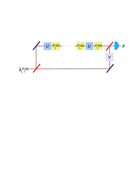
Figure 1: Interferometric approach to obtain the holonomy $\boldsymbol{U}_{g}^{(\kappa)}[\mathcal{C}_{l_{1}},\ldots,\mathcal{C}_{l_{\kappa}}]$. The horizontal and vertical paths of the Mach-Zehnder interferometer correspond to the states $|0\rangle$ and $|1\rangle$, respectively. The particle have an internal degree of freedom, on which the unitary operation $U$ is applied. $U$ can be generated either by adiabatic or nonadiabatic evolution, or approximated by filtering measurements. The particle enters the interferometer in path $0$ and in the internal state $P_{l_{1}}(0)/n_{l_{1}}$. In path $1$ a variable unitary operator $V$ such that $[V,P_{l}(0)]=0$, $\forall l$, is applied, while in path $0$ we alternatingly apply $U$ and a filtering corresponding to the projector $|0\rangle\langle 0|\otimes P_{l_{k}}(0)+|1\rangle\langle 1|\otimes\hat{1}$, for $k=2,\ldots\kappa$. A final $U$ is applied, followed by the filtering $|0\rangle\langle 0|\otimes P_{l_{1}}(0)+|1\rangle\langle 1|\otimes\hat{1}$. The probability $p$ to find the particle in path $0$ is measured after a second beam splitter. The unitary operator $V$ is varied so as to maximize $p$.

Let us now examine some possible physical realizations of $\boldsymbol{U}_{g}^{(\kappa)}[\mathcal{C}_{l_{1}},\ldots,\mathcal{C}_{l_{\kappa}}]$. Consider the Mach-Zehnder interferometer in fig. 1 with the two path states represented by $|0\rangle$ and $|1\rangle$. We let the internal state of the particle (e.g., spin) be represented by the Hilbert space $\mathcal{H}=\mathcal{H}_{1}(s)\oplus\cdots\oplus\mathcal{H}_{\eta}(s)$, $s\in[0,1]$. The total system is prepared in the state $|0\rangle\langle 0|\otimes P_{l_{1}}(0)/n_{l_{1}}$. We first apply a beam-splitter, followed by the unitary operations $|0\rangle\langle 0|\otimes\hat{1}+|1\rangle\langle 1|\otimes V$ and $|0\rangle\langle 0|\otimes U+|1\rangle\langle 1|\otimes\hat{1}$, where $V$ is a variable unitary operator assumed to be chosen such that $[V,P_{l}(0)]=0$ for all $l$. Next, we perform a filtering corresponding to the projection operator $|0\rangle\langle 0|\otimes P_{l_{2}}(0)+|1\rangle\langle 1|\otimes\hat{1}$, i.e., the particle is “removed” if it is found in path $0$ with its internal state outside subspace $\mathcal{H}_{l_{2}}$. Thereafter, we again apply the operator $|0\rangle\langle 0|\otimes U+|1\rangle\langle 1|\otimes\hat{1}$, and the filtering $|0\rangle\langle 0|\otimes P_{l_{3}}(0)+|1\rangle\langle 1|\otimes\hat{1}$. This procedure is repeated until we have applied the operator $|0\rangle\langle 0|\otimes U+|1\rangle\langle 1|\otimes\hat{1}$, $\kappa$ times. After this, we apply a final filtering $|0\rangle\langle 0|\otimes P_{l_{1}}(0)+|1\rangle\langle 1|\otimes\hat{1}$, and recombine the two paths with a beam splitter. We finally measure the probability $p$ to find the particle in path $0$.

First, we assume that the unitary operator $U$ acting on $\mathcal{H}$ is caused by an adiabatic evolution of a time-dependent Hamiltonian with eigenspaces $\{\mathcal{H}_{l}(s)\}_{l=1}^{\eta}$. This allows us to write $U=\sum_{l}e^{i\phi_{l}}\Gamma_{l}$, where $\phi_{l}$ is the dynamical phase $\phi_{l}=\int_{0}^{1}E_{l}(s)ds$, and $E_{l}(s)$ the eigenvalue corresponding to eigenspace $\mathcal{H}_{l}(s)$ of the Hamiltonian. The corresponding detection probability becomes

$$p = \frac{1}{4}+\frac{1}{4}\frac{1}{n_{l_{1}}}{\textrm{Tr}}(\gamma_{l_{1}\ldots l_{\kappa}}\gamma_{l_{1}\ldots l_{\kappa}}^{\dagger})$$ (14)

$$+\frac{1}{2}\frac{1}{n_{l_{1}}}{\textrm{Re}}[e^{i\sum_{k=1}^{\kappa}\phi_{k}}{\textrm{Tr}}(\boldsymbol{\gamma}^{l_{1}\ldots l_{\kappa}}\boldsymbol{V}^{\dagger})],$$

where $\boldsymbol{V}_{ij}=\langle l_{1}^{i}(0)|V|l_{1}^{j}(0)\rangle$. Note that $\boldsymbol{V}$ is a unitary matrix since $[V,P_{l_{1}}(0)]=0$. By varying $V$ we obtain the maximal detection probability when $\boldsymbol{V}=e^{i\sum_{k=1}^{\kappa}\phi_{k}}\boldsymbol{U}_{g}^{(\kappa)}[\mathcal{C}_{l_{1}},\ldots,\mathcal{C}_{l_{\kappa}}]$. Hence, up to the dynamical phases we have found the holonomy.

In the adiabatic setting there is in the general case no easy way to eliminate the dynamical phases. To avoid these problems we consider two alternative approaches to generate the unitary operator $U$. One alternative is to base the evolution entirely on filtering, where we approximate the evolution in the spirit of ref. sjoqvist06 . We begin with the same initial state, beam-splitter, and variable unitary $V$, as in the previous case. Next we apply a sequence of filterings $|0\rangle\langle 0|\otimes P_{l_{1}}(s_{j})+|1\rangle\langle 1|\otimes\hat{1}$, where $s_{j}$ form a discretization of the interval $[0,1]$. For the next step we apply the sequence of filterings $|0\rangle\langle 0|\otimes P_{l_{2}}(s_{j})+|1\rangle\langle 1|\otimes\hat{1}$, and we continue up $l_{\kappa}$. We finally apply $|0\rangle\langle 0|\otimes P_{l_{1}}(0)+|1\rangle\langle 1|\otimes\hat{1}$, followed by a beam splitter, and measure the probability to find the particle in path $0$. One can show that the probability is

$$p = \frac{1}{4}+\frac{1}{4}\frac{1}{n_{l_{1}}}{\textrm{Tr}}(\gamma_{l_{1}\ldots l_{\kappa}}\gamma_{l_{1}\ldots l_{\kappa}}^{\dagger})$$ (15)

$$+\frac{1}{2}\frac{1}{n_{l_{1}}}{\textrm{Re}}[{\textrm{Tr}}(\boldsymbol{\gamma}^{l_{1}\ldots l_{\kappa}}\boldsymbol{V}^{\dagger})].$$

Hence, as in eq. (14), apart from the absence of dynamical phases.

The second alternative that allows us to avoid the problem with dynamical phases is to use a nonadiabatic approach. Assume that the evolution is driven by the time-dependent Hamiltonian $H(s)$, where now $s$ is the time-parameter. We let the subspaces $\mathcal{H}_{l}(s)$ be evolving under $H(s)$ according to the Schrödinger equation. In contrast to the adiabatic approach the subspaces $\mathcal{H}_{l}(s)$ are in the general case not eigenspaces of $H(s)$. We furthermore let $\{|l^{j}(s)\rangle\}_{j=1}^{n_{l}}$ be smoothly parameterized orthonormal bases of the subspaces $\mathcal{H}_{l}(s)$. We wish to find the unitary matrices $\boldsymbol{U}_{l}(s)$ such that the vectors

$$|\chi_{l}^{k}(s)\rangle=\sum_{j}|l^{j}(s)\rangle[\boldsymbol{U}_{l}(s)]_{jk}$$ (16)

satisfy the Schrödinger equation $i\partial_{s}|\chi_{l}^{k}(s)\rangle=H(s)|\chi_{l}^{k}(s)\rangle$ ($\hbar=1$) with initial conditions $|\chi_{l}^{k}(0)\rangle=|l^{k}(0)\rangle$. If we substitute eq. (16) into the Schrödinger equation we find that $\boldsymbol{U}_{l}(s)$ has to satisfy $i\partial_{s}\boldsymbol{U}_{l}(s)=i\boldsymbol{A}_{l}(s)\boldsymbol{U}_{l}(s)+\boldsymbol{K}_{l}(s)\boldsymbol{U}_{l}(s)$, where $[\boldsymbol{A}_{l}(s)]_{j^{\prime}j}=\langle\partial_{s}l^{j^{\prime}}(s)|l^{j}(s)\rangle$ and $[\boldsymbol{K}_{l}(s)]_{j^{\prime}j}=\langle l^{j^{\prime}}(s)|H(s)|l^{j}(s)\rangle$ contain the geometrical and dynamical contributions, respectively, as was discussed in ref. anandan88 . In order to get rid of the dynamical contribution without affecting the evolution of the subspaces we introduce the modified time-dependent Hamiltonian

$$\overline{H}(s)=H(s)-\sum_{l=1}^{\eta}P_{l}(s)H(s)P_{l}(s).$$ (17)

The evolution of the subspaces $\mathcal{H}_{l}(s)$ are not affected by this modification since $[\overline{H}(s),P_{l}(s)]=[H(s),P_{l}(s)]$, $\forall l$. We now wish to find the unitary matrices $\overline{\boldsymbol{U}}_{l}(s)$ such that the vectors $|\overline{\chi}^{k}_{l}(s)\rangle=\sum_{j}|l^{j}(s)\rangle[\overline{\boldsymbol{U}}_{l}(s)]_{jk}$ satisfy the modified Schrödinger equation $i\partial_{t}|\overline{\chi}^{k}_{l}(s)\rangle=\overline{H}(s)|\overline{\chi}^{k}_{l}(s)\rangle=[H(s)-P_{l}(s)H(s)P_{l}(s)]|\overline{\chi}^{k}_{l}(s)\rangle$ with initial conditions $|\overline{\chi}^{k}_{l}(0)\rangle=|l^{k}(0)\rangle$. In this case we obtain $\partial_{s}\overline{\boldsymbol{U}}_{l}(s)=i\boldsymbol{A}_{l}(s)\overline{\boldsymbol{U}}_{l}(s)$. Hence, the solution $\overline{\boldsymbol{U}}_{l}(s)={\bf P}e^{\int_{0}^{s}\boldsymbol{A}_{l}(s^{\prime})ds^{\prime}}$ only depends on the geometric contribution. The time-dependent Hamiltonian $\overline{H}(s)$ generates a unitary mapping from the initial state to the state at time $s=1$ that is given by $\overline{U}(1)=\sum_{l}\Gamma_{l}$, where

$$\Gamma_{l} = \sum_{k}|\overline{\chi}^{k}_{l}(1)\rangle\langle\overline{\chi}^{k}_{l}(0)|$$ (18)

$$= \sum_{jk}[{\bf P}e^{\int_{0}^{1}\boldsymbol{A}(s)ds}]_{jk}|l^{j}(1)\rangle\langle l^{k}(0)|.$$

This means that if we let $U=\overline{U}(1)$ in the alternating procedure described above (see fig. 1), then the probability to detect the particle in path $0$ becomes as in eq. (15), and is maximized when $\boldsymbol{V}=\boldsymbol{U}_{g}^{(\kappa)}[\mathcal{C}_{l_{1}},\ldots,\mathcal{C}_{l_{\kappa}}]$.

VI Conclusion

Noncyclic evolution of quantum systems may lead to well-defined off-diagonal holonomies that involve more than one subspace of Hilbert space. These holonomies reduce to the off-diagonal geometric phases in ref. manini00 for one-dimensional subspaces. The off-diagonal holonomies are undefined for cyclic evolution but must contain members of nonzero rank when all the standard holonomies are undefined. While the nodal point structure of the holonomy for an open continuous path kult06 can only depend on the end-points of the path, this structure can be path-dependent in the off-diagonal case. Furthermore, we have put forward physical realizations of the off-diagonal holonomies in the context of adiabatic evolution and interferometry that may open up the possibility to test these quantities experimentally.

References

• (1) SAMUEL J. and BHANDARI R., Phys. Rev. Lett., 60 (1988) 2339.
• (2) BHANDARI R., Phys. Lett. A, 157 (1991) 221.
• (3) BHANDARI R., Phys. Lett. A, 171 (1992) 262.
• (4) BHANDARI R., Phys. Lett. A, 171 (1992) 267.
• (5) BHANDARI R., Phys. Lett. A, 180 (1993) 15.
• (6) MANINI N. and PISTOLESI F., Phys. Rev. Lett., 85 (2000) 3067.
• (7) MUKUNDA N., ARVIND, CHATURVEDI S. and SIMON R., Phys. Rev. A, 65 (2002) 012102.
• (8) HASEGAWA Y., LOIDL R., BARON M., BADUREK G. and RAUCH H., Phys Rev. Lett., 87 (2001) 070401.
• (9) HASEGAWA Y., LOIDL R., BADUREK G., BARON M., MANINI N., PISTOLESI F. and RAUCH H., Phys Rev. A, 65 (2002) 052111.
• (10) FILIPP S. and SJÖQVIST E., Phys. Rev. Lett., 90 (2003) 050403 (2003).
• (11) FILIPP S. and SJÖQVIST E., Phys. Rev. A, 68 (2003) 042112.
• (12) TONG D. M., SJÖQVIST E., FILIPP S., KWEK L. C. and OH C. H., Phys. Rev. A, 71 (2005) 032106.
• (13) FILIPP S. and SJÖQVIST E., Phys. Lett. A, 342 (2005) 205.
• (14) WILCZEK F. and ZEE A., Phys. Rev. Lett., 52 (1984) 2111.
• (15) ZANARDI P. and RASETTI M., Phys. Lett. A, 264 (1999) 94.
• (16) PACHOS J., ZANARDI P. and RASETTI M., Phys. Rev. A, 61 (2000) 010305(R).
• (17) PACHOS J. and CHOUNTASIS S., Phys. Rev. A, 62 (2000) 052318.
• (18) DUAN L. -M., CIRAC J. I. and ZOLLER P., Science, 292 (2001) 1695.
• (19) RECATI A., CALARCO T., ZANARDI P., CIRAC J. I. and ZOLLER P., Phys. Rev. A, 66 (2002) 032309.
• (20) FAORO L., SIEWERT J. and FAZIO R., Phys. Rev. Lett., 90 (2003) 028301.
• (21) ANANDAN J., Phys. Lett. A, 133 (1988) 171.
• (22) SJÖQVIST E., KULT D. and ÅBERG J., Phys. Rev. A, 74 (2006) 062101.
• (23) MOSTAFAZADEH A., J. Phys. A, 32 (1999) 8157.
• (24) KULT D., ÅBERG J. and SJÖQVIST E., Phys. Rev. A, 74 (2006) 022106.
• (25) GREUB W., HALPERIN S. and VANSTONE R., Connections, Curvature and Cohomology Vol. II (Academic Press, New York) 1973.
• (26) MOORE E. H., Bull. Am. Math. Soc., 26 (1920) 394.
• (27) PENROSE R., Proc. Cambridge Phil. Soc., 51 (1955) 406.
• (28) LANCASTER P. and TISMENETSKY M., The Theory of Matrices (Academic Press, San Diego) 1985.
• (29) MARCUS M. and MINC H., A Survey of Matrix Theory and Matrix Inequalities (Allyn and Bacon, Inc, Boston) 1964.
• (30) UNANYAN R. G., SHORE B. W. and BERGMANN K., Phys. Rev. A, 59 (1999) 2910.