Continuous-Variable Quantum Cloning of Coherent states with Phase-Conjugate Input Modes Using Linear Optics

Abstract

We propose a scheme for continuous-variable quantum cloning of coherent states with phase-conjugate input modes using linear optics. The quantum cloning machine yields $M$ identical optimal clones from $N$ replicas of a coherent state and $N$ its replicas of phase conjugate. This scheme can be straightforwardly implemented with the setup accessible at present since its optical implementation only employs simple linear optical elements and homodyne detection. Compared with the original scheme for continuous variables quantum cloning with phase-conjugate input modes proposed by Cerf and Iblisdir [Phys. Rev. Lett. 87, 247903 (2001)], which utilized a nondegenerate optical parametric amplifier, our scheme loses the output of phase-conjugate clones and is regarded as irreversible quantum cloning.

I Introduction

Quantum cloning plays an important role in quantum information and quantum communication. It has been shown that quantum cloning might improve the performance of some computational tasks one and it is believed to be the optimal eavesdropping attack for a certain class of quantum cryptography two . It also opens an avenue for understanding the concepts of quantum mechanics and measurement theory further. So the quantum cloning which achieves the optimal cloning transformation compatible with the quantum no cloning theorem has always being a hot research topic. Such a quantum cloning machine was first considered by Buzek and Hillery for qubits three and later extended to the continuous-variable (CV) regime by Cerf et al. four . CV quantum cloning has been extensively studied in the recent years for the relative ease in preparing and manipulating quantum states. The theoretical proposals for the experimental implementations of CV quantum cloning have been proposed five ; six ; seven ; seven1 .

A recent result in the context of measurement has revealed that more quantum information can be encoded in the antiparallel pairs of spins than parallel pairs eight . Subsequently, a result that a pair of conjugate Gaussian states can carry more information than by using the same states twice has been extended to continuous variables nine . This result makes it possible to yield better fidelity with the cloning machine admitting antiparallel input qubits or phase-conjugate input modes thereby opening a new avenue in the investigation of quantum cloning. Based on the above properties, Cerf and Iblisdir put forward a CV cloning transformation ten that takes as input $N$ replicas of a coherent states and $N^{{}^{\prime}}$ replicas of its complex conjugate, and produces $M$ optimal clones of the coherent state and $M^{\prime}=M+N^{\prime}-N$ phase-conjugate clones (anticlones, or time reversed states). This is the first scheme for the phase-conjugate input (PCI) cloner of continuous variables. It is, nonetheless, difficult for the practical experimental realization of the proposed PCI cloner due to the difficulties associated with the physical implementation of the optical parametric amplifier. Recently, a much simpler but efficient CV quantum cloning machine based on linear optics and homodyne detection was proposed and realized experimentally by Andersen et al. eleven . Later, this protocol is extended to various quantum cloning cases, such as asymmetric cloning eleven1 and so on twelve . According to classifying the quantum clone to irreversible and reversible types in the perspective of quantum information distribution teleclone , the quantum cloning with linear optics eleven is local and irreversible, in which the anticlones are lost. Perfect distribution do not allow losing any the quantum information of the transmitted unknown state, that means this process is reversible and the unknown state can be reconstructed in a quantum system again.

In this paper, we propose a protocol of CV quantum cloning of coherent states with phase-conjugate input modes using linear optics. The $N+N\rightarrow M$ quantum cloning machine yields $M$ identical optimal clones from $N$ replicas of a coherent state and $N$ its replicas of phase conjugate. This scheme is regarded as local and irreversible PCI quantum cloning because the anticlones are lost. We also show that $N+N\rightarrow M$ irreversible PCI quantum cloning machine may be changed into $N+N\rightarrow M+M$ reversible PCI quantum cloning machine by the introduction of an EPR (Einstein-Podolsky-Rosen) entangled ancilla. It shows that the optimal fidelity of the anticlones requires the maximally EPR entangled state.

II $1+1\rightarrow M$ Irreversible PCI Quantum Cloning

The quantum states we consider in this paper are described with the electromagnetic field annihilation operator $\hat{a}=(\hat{X}+i\hat{P})/2$, which is expressed in terms of the amplitude $\hat{X}$ and phase $\hat{P}$ quadrature with the canonical commutation relation $[\hat{X},\hat{P}]=2i$. Without any loss of generality, the quadrature operators can be expressed in terms of a steady state and fluctuating component as $\hat{A}=\langle\hat{A}\rangle+\Delta\hat{A}$, which have variances of $V_{A}=\langle\Delta\hat{A}^{2}\rangle$ ($\hat{A}=\hat{X}$ or $\hat{P})$. The input coherent state and its phase-conjugate state to be cloned will be described by $\left|\alpha_{in}\right\rangle=\left|\frac{1}{2}\left(x_{in}+ip_{in}\right)\right\rangle$ and $\left|\alpha_{in}^{*}\right\rangle=\left|\frac{1}{2}\left(x_{in}-ip_{in}\right)\right\rangle$ respectively, where $x_{in}$ and $p_{in}$ are the expectation values of $\hat{X}_{in}$ and $\hat{P}_{in}$. The cloning machine generates many clones of input state characterized by the density operator $\hat{\rho}_{clone}$ and the expectation $x_{clone}$ and $p_{clone}$. The quality of the cloning machine can be quantified by the fidelity, which a overlap between the input state and the output state. It is defined by fifteen

$$F = \left\langle\alpha_{in}\right|\hat{\rho}_{clone}\left|\alpha_{in}\right\rangle=\frac{2}{\sqrt{(1+\Delta^{2}\hat{X}_{clone})(1+\Delta^{2}\hat{P}_{clone})}}$$ (1)

$$*\exp\left[-\frac{(x_{clone}-x_{in})^{2}}{2(1+\Delta^{2}\hat{X}_{clone})}-\frac{(y_{clone}-y_{in})^{2}}{2(1+\Delta^{2}\hat{P}_{clone})}\right]$$

In the case of unity gains, i.e., $x_{clone}=x_{in}$, the fidelity is strongly peaked and changed into

$$F=\frac{2}{\sqrt{(1+\Delta^{2}\hat{X}_{clone})(1+\Delta^{2}\hat{P}_{clone})}}.$$ (2)

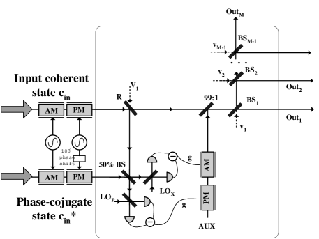
Figure 1: A schematic diagram of $1+1\rightarrow M$ irreversible PCI quantum cloning. BS: Beam splitter, LO: Local oscillator, AM: Amplitude modulator, PM: Phase modulator and AUX: Auxiliary beam.

Let us first illustrate the protocol in the simplest case of $N=N^{\prime}=1$ as shown in Fig. 1. The input coherent state $\hat{c}_{in}$ and its phase-conjugate state $\hat{c}_{in}^{*}$ are prepared by an amplitude modulator and a phase modulator respectively. The modulated signals on the amplitude modulators are in-phase and the modulated signals on the phase modulators are out–of-phase. The input mode $\hat{c}_{in}$ is divided by a variable beam splitter with transmission rate $T$ and reflectivity rate $R$. The reflected output $\hat{c}_{1r}=\sqrt{R}\hat{c}_{in}+\sqrt{T}\hat{V}_{1}$, where the annihilation operator $\hat{V}_{1}$ represents the vacuum mode entering the beam splitter, is combined with its phase-conjugate state $\hat{c}_{in}^{*}$ at a 50/50 beam splitter. Then we perform homodyne measurements on the two output beams to achieve the amplitude and the phase quadratures simultaneously. The measured quadratures are

$$\hat{X}_{m} = \frac{1}{\sqrt{2}}(\sqrt{R}\hat{X}_{c_{in}}+\sqrt{T}\hat{X}_{V_{1}}+\hat{X}_{c_{in}^{*}})$$

$$\hat{P}_{m} = \frac{1}{\sqrt{2}}(\sqrt{R}\hat{P}_{c_{in}}+\sqrt{T}\hat{P}_{V_{1}}-\hat{P}_{c_{in}^{*}}).$$ (3)

We use the measurement outcomes to modulate the amplitude and phase of an auxiliary coherent beam via two independent modulators with a scaling factor $g$ sixteen . This beam is then combined at a 99/1 beam splitter with the transmitted part of mode $\hat{c}_{in}$, hereby displacing this part according to the measurement outcomes sixteen . Corresponding to the transformation $\hat{A}\rightarrow\hat{D}^{+}\hat{A}\hat{D}=\hat{A}+\left(\hat{X}_{m}+i\hat{P}_{m}\right)/2$ in the Heisenberg representation, the displaced field can be expressed as

$$\hat{c}_{disp} = (\sqrt{1-R}+\frac{g}{\sqrt{2}}\sqrt{R})\hat{c}_{in}$$ (4)

$$-(\sqrt{R}-\frac{g}{\sqrt{2}}\sqrt{1-R})\hat{V}_{1}+\frac{g}{\sqrt{2}}\hat{c}_{in}^{*+}$$

where $\hat{c}_{disp}$ is the annihilation operator for the displaced field. By choosing $g=\sqrt{2R/\left(1-R\right)}$, we can cancel the vacuum noise of the displaced field. Then the displaced field is given by

$$\hat{c}_{disp}^{c}=\frac{1}{\sqrt{1-R}}\hat{c}_{in}+\frac{\sqrt{R}}{\sqrt{1-R}}\hat{c}_{in}^{*+}.$$ (5)

We can see Eq. (5) equal to a phase-insensitive amplification with gain $G=\frac{1}{1-R}$.

In the final step the displaced field is distributed into $M$ clones $\{\hat{a}_{l}^{{}^{\prime}}\}$ $(l=1,2,\cdots M$ $)$ by a sequence of $M-1$ beam splitters with appropriately adjusted transmittances and reflectances. Then the output of cloning machine can be expressed by

$$\hat{a}_{1}^{{}^{\prime}} = \sqrt{\frac{1}{M}}\hat{c}_{disp}^{c}+\sqrt{\frac{M-1}{M}}\hat{v}_{1}$$

$$\hat{a}_{2}^{{}^{\prime}} = \sqrt{\frac{1}{M}}\hat{c}_{disp}^{c}-\sqrt{\frac{1}{M\left(M-1\right)}}\hat{v}_{1}+\sqrt{\frac{M-2}{M-1}}\hat{v}_{2}$$

$$\cdots$$

$$\hat{a}_{M-1}^{{}^{\prime}} = \sqrt{\frac{1}{M}}\hat{c}_{disp}^{c}-\sqrt{\frac{1}{M\left(M-1\right)}}\hat{v}_{1}-\sqrt{\frac{1}{\left(M-1\right)\left(M-2\right)}}$$

$$*\hat{v}_{2}-\cdots-\sqrt{\frac{1}{3*2}}\hat{v}_{\left(M-2\right)}+\sqrt{\frac{1}{2}}\hat{v}_{\left(M-1\right)}$$

$$\hat{a}_{M}^{{}^{\prime}} = \sqrt{\frac{1}{M}}\hat{c}_{disp}^{c}-\sqrt{\frac{1}{M\left(M-1\right)}}\hat{v}_{1}-\sqrt{\frac{1}{\left(M-1\right)\left(M-2\right)}}$$ (6)

$$*\hat{v}_{2}-\cdots-\sqrt{\frac{1}{3*2}}\hat{v}_{\left(M-2\right)}-\sqrt{\frac{1}{2}}\hat{v}_{\left(M-1\right)}$$

where $\hat{v}_{k}\left(k=1,2,\cdots M-1\right)$ refer to the annihilation operators of vacuum mode entering the $BS_{1},BS_{2},\cdots BS_{M-1}$ respectively. Eq. (6) shows that each output mode contains the in the displaced field $\hat{c}_{disp}^{c}$ with a factor of $1/\sqrt{M}$. Note that both terms $\hat{c}_{in}$ and $\hat{c}_{in}^{*+}$ in the Eq. (5) contribute to the total coherent signal with a factor of $1/\sqrt{1-R}+\sqrt{R}/\sqrt{1-R}$ and noise variances with $\sqrt{1+R}/\sqrt{1-R}$ in the output $\hat{c}_{disp}^{c}$. Since each output cloner should includes one unit of the input coherent state, the $R$ must satisfy

$$\frac{1}{\sqrt{1-R}}+\frac{\sqrt{R}}{\sqrt{1-R}}=\sqrt{M}.$$ (7)

The $R$ can be easily determined by solving the above equation and given by

$$R=\frac{\left(M-1\right)^{2}}{\left(M+1\right)^{2}}.$$ (8)

According to the Eqs. (5,6,8), the variances of the clones can be written as

$$\Delta^{2}\hat{X}_{a_{l}^{{}^{\prime}}} = \Delta^{2}\hat{P}_{a_{l}^{{}^{\prime}}}=\frac{1}{M}\frac{1+R}{1-R}+\frac{M-1}{M}$$

$$= 1+\frac{\left(M-1\right)^{2}}{2M^{2}}.$$

The fidelity can be get through Eq. (2)

$$F_{\left({}_{1}^{1}\right)\rightarrow M}=\frac{4M^{2}}{4M^{2}+\left(M-1\right)^{2}}.$$ (10)

This procedure is optimal clearly to produce $M$ clones. Now we compare the fidelity of $M$ clones from the phase-conjugate input modes with from the two identical replicas. The fidelity of the standard 2-to-M cloning are given by seventeen

$$F_{2\rightarrow M}=\frac{2M}{3M-2}$$ (11)

In the special case $M=2$, the standard cloning can be achieved perfectly with fidelity equal to one while the phase-conjugate cloner yields an additional variance which will lead to a lower fidelity. It is, nonetheless, obvious that phase-conjugate cloner yields better fidelity than the standard cloning when $M\geq 3$. In the limit of large $M\rightarrow\infty$, we could see $F_{\left({}_{1}^{1}\right)\rightarrow\infty}=\frac{4}{5}$ compared with the standard cloning $F_{2\rightarrow\infty}=\frac{2}{3}$. This shows that more information can be encoded into a pair of conjugate Gaussian states than by using the two same states, which has been shown in Ref. nine . Compared with the original scheme for continuous variables quantum cloning with phase-conjugate input modes proposed by Cerf and Iblisdir ten , which utilized a nondegenerate optical parametric amplifier, our scheme loses the anticlones and is regarded as irreversible PCI quantum cloning.

Now we consider the realistic conditions where the homodyne detector efficiency is not unity. If $\eta$ expresses the homodyne detector efficiency, the measured amplitude and the phase quadratures are give by

$$\hat{X}_{m} = \sqrt{\frac{\eta}{2}}(\sqrt{R}\hat{X}_{c_{in}}+\sqrt{T}\hat{X}_{V_{1}}+\hat{X}_{c_{in}^{*}})+\sqrt{1-\eta}\hat{X}_{V_{D1}}$$

$$\hat{P}_{m} = \sqrt{\frac{\eta}{2}}(\sqrt{R}\hat{P}_{c_{in}}+\sqrt{T}\hat{P}_{V_{1}}-\hat{P}_{c_{in}^{*}})+\sqrt{1-\eta}\hat{P}_{V_{D2}}$$ (12)

where $\hat{X}_{V_{D1}}$ and $\hat{P}_{V_{D2}}$ are the vacuum noise introduced from the losses of the homodyne detector. With the measured results, the displaced field can be expressed as

$$\hat{c}_{disp} = (\sqrt{1-R}+g\sqrt{\frac{\eta}{2}}\sqrt{R})\hat{c}_{in}-(\sqrt{R}-g\sqrt{\frac{\eta}{2}}\sqrt{1-R})\hat{V}_{1}$$ (13)

$$+g\sqrt{\frac{\eta}{2}}\hat{c}_{in}^{*+}+\sqrt{1-\eta}g\hat{X}_{V_{D1}}+\sqrt{1-\eta}g\hat{P}_{V_{D2}}$$

By choosing $g=\sqrt{2R/\eta(1-R)}$, the displaced field is given by

$$\hat{c}_{disp}^{c} = \frac{1}{\sqrt{1-R}}\hat{c}_{in}+\frac{\sqrt{R}}{\sqrt{1-R}}\hat{c}_{in}^{*+}$$ (14)

$$+\sqrt{\frac{2R(1-\eta)}{(1-R)\eta}}(\hat{X}_{V_{D1}}+\hat{P}_{V_{D2}}).$$

According to the Eqs. (6,7,8), the variances of the clones can be written as

$$\Delta^{2}\hat{X}_{a_{l}^{{}^{\prime}}}=\Delta^{2}\hat{P}_{a_{l}^{{}^{\prime}}} = \frac{1}{M}\frac{1+R}{1-R}+\frac{1}{M}\frac{2R(1-\eta)}{(1-R)\eta}$$ (15)

$$+\frac{M-1}{M} = 1+\frac{1}{\eta}\frac{\left(M-1\right)^{2}}{2M^{2}}.$$

The fidelity can be get through Eq. (2)

$$F_{\left({}_{1}^{1}\right)\rightarrow M}=\frac{4\eta M^{2}}{4\eta M^{2}+\left(M-1\right)^{2}}.$$ (16)

It clearly shows that the fidelity of the clones is degraded due to the losses of the homodyne detection.

III $N+N\rightarrow M$ Irreversible PCI Quantum Cloning

We now generalize $1+1\rightarrow M$ case to $N+N\rightarrow M$ irreversible PCI quantum cloning, which produces $M$ clones from input $N$ replicas of a coherent states and $N$ replicas of its complex conjugate as illustrated in Fig. 2. First, we concentrate $N$ identically prepared coherent states $\left|\Phi\right\rangle$ described by $\left\{\hat{a}_{l}\right\}$ $(l=1,\cdots N)$ into a single spatial mode $\hat{c}_{1}$ with amplitude $\sqrt{N}\Phi$. This operation can be performed by interfering $N$ input modes in $N-1$ beam splitters, which yields the mode

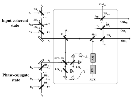
Figure 2: A schematic diagram of $N+N\rightarrow M$ irreversible PCI quantum cloning.

$$\hat{c}_{1}=\frac{1}{\sqrt{N}}\sum_{l=1}^{N}\hat{a}_{l}$$ (17)

and $N-1$ vacuum modes. The same method can be used on the generation of the phase-conjugate input mode $\hat{c}_{2}$ with amplitude $\sqrt{N}\Phi^{*}$ from the $N\$replicas of $\left|\Phi^{*}\right\rangle$ stored in the $N\$modes $\left\{b_{l}\right\}$ $(l=1,\cdots N)$, which is expressed as

$$\hat{c}_{2}=\frac{1}{\sqrt{N}}\sum_{l=1}^{N}\hat{b}_{l}.$$ (18)

Then, $\hat{c}_{1}$ and $\hat{c}_{2}$ is transported into the cloning machine same as Fig. 1. The displaced field is given by

$$\hat{c}_{disp}^{c}=\frac{1}{\sqrt{1-R}}\hat{c}_{1}+\frac{\sqrt{R}}{\sqrt{1-R}}\hat{c}_{2}^{+}.$$ (19)

The terms $\hat{c}_{1}$ and $\hat{c}_{2}^{+}$ in the Eq. (19) contribute to the total coherent signal with a factor of $\sqrt{N}(1/\sqrt{1-R}+\sqrt{R}/\sqrt{1-R})$ and noise variances with $(1+R)/(1-R)$ in the output $\hat{c}_{disp}^{c}$. Since each output cloner should includes one unit of the input coherent state, the $R$ must satisfy

$$\sqrt{N}(\frac{1}{\sqrt{1-R}}+\frac{\sqrt{R}}{\sqrt{1-R}})=\sqrt{M}.$$ (20)

The $R$ can be easily determined by solving the above equation and given by

$$R=\frac{\left(M-N\right)^{2}}{\left(M+N\right)^{2}}.$$ (21)

The variance and fidelity of $\left({}_{N}^{N}\right)\rightarrow$ $M$ cloner will be given by

$$\Delta^{2}\hat{X}_{a_{l}^{{}^{\prime}}}=\Delta^{2}\hat{P}_{a_{l}^{{}^{\prime}}}=1+\frac{\left(M-N\right)^{2}}{2M^{2}N},$$ (22)

$$F_{\left({}_{N}^{N}\right)\rightarrow M}=\frac{4M^{2}N}{4M^{2}N+\left(M-N\right)^{2}}.$$ (23)

Obviously, Eqs. (II) and (10) can be obtained by Eqs. (22) and (23) for $N=N^{\prime}=1$. The result also coincides with that obtained in Ref. ten . However, the output anticlones are lost in this scheme. The advantage of dealing with $N\$pair of complex conjugate inputs can still be most easily illustrated in the limit of infinite number of clones, $M\rightarrow\infty$ , from Eq. (23) we get $F_{{}_{\left({}_{N}^{N}\right)\rightarrow M}}=\frac{4N}{4N+1}$ while the standard cloning machine fidelity $F_{2N\rightarrow M}=\frac{2N}{2N+1}$.

IV Reversible PCI Cloning with Linear Optics and EPR Entanglement

A scheme for a phase conjugating amplifier with the nonlinearity put off-line was proposed eighteen . Employing this protocol, we show that $N+N\rightarrow M$ irreversible PCI quantum cloning machine as shown in Fig. 2 become $N+N\rightarrow M+M$ reversible PCI quantum cloning machine by the introduction of an EPR entangled ancilla (two-mode Gaussian entangled state) as shown Fig. 3. One half of the entangled ancilla is injected into the empty port of the variable beam splitter. Since the noises injected into the empty port of the variable beam splitter are canceled in the displaced field, the displaced field don’t depend on the injected noises. Thus the above results for the clones are always valid. The other half of the entangled ancilla is also displaced according to the classical measurement outcomes with a scaling factor $g_{1}$ and expressed as

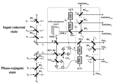
Figure 3: A schematic diagram of reversible PCI cloning with linear optics and EPR entanglement.

$$\hat{e}_{disp}=\frac{g_{1}}{\sqrt{2}}\sqrt{R}\hat{c}_{1}^{+}+\frac{g_{1}}{\sqrt{2}}\sqrt{1-R}\hat{b}_{EPR1}^{+}+\hat{b}_{EPR2}+\frac{g_{1}}{\sqrt{2}}\hat{c}_{2}.$$ (24)

By choosing $g_{1}=\sqrt{2/\left(1-R\right)}$, the displaced EPR beam is given by

$$\hat{e}_{disp}=\frac{\sqrt{R}}{\sqrt{1-R}}\hat{c}_{1}^{+}+\frac{1}{\sqrt{1-R}}\hat{c}_{2}+(\hat{b}_{EPR1}^{+}+\hat{b}_{EPR2}).$$ (25)

The EPR entangled beams $\hat{b}_{EPR1}$, $\hat{b}_{EPR2}$ have the very strong correlation property, such as both their sum-amplitude quadrature variance $\langle\Delta(\hat{X}_{b_{EPR1}}+\hat{X}_{b_{EPR2}})^{2}\rangle=2e^{-2r}$, and their difference-phase quadrature variance $\langle\Delta(\hat{Y}_{b_{EPR1}}-\hat{Y}_{b_{EPR2}})^{2}\rangle=2e^{-2r}$, are less than quantum noise limit. In the final step the displaced EPR beam is distributed into $M$ anticlones $\{\hat{b}_{l}^{{}^{\prime}}\}$ $(l=1,2,\cdots M$ $)$ by a sequence of $M-1$ beam splitters with appropriately adjusted transmittances and reflectances. The expression of the output anticlones is similar to Eq. 6. The variance and fidelity of anticloner will be given by

$$\Delta^{2}\hat{X}_{b_{l}^{{}^{\prime}}}=\Delta^{2}\hat{P}_{b_{l}^{{}^{\prime}}}=1+\frac{\left(M-N\right)^{2}}{2M^{2}N}+\frac{2e^{-2r}}{M},$$ (26)

$$F_{\left({}_{N}^{N}\right)\rightarrow M}^{anti}=\frac{4M^{2}N}{4M^{2}N+\left(M-N\right)^{2}+4MNe^{-2r}}.$$ (27)

It clearly shows that the optimal fidelity of the anticlones requires the maximally EPR entangled state $r\rightarrow\infty$. Clearly the reversible PCI cloning with linear optics and EPR entanglement is equivalent to the original scheme for CV PCI quantum cloning proposed by Cerf and Iblisdir ten , which utilized a nondegenerate optical parametric amplifier.

V Conclusion  

In conclusion, we have proposed a much simpler and experimentally feasible continuous variables cloning machine of coherent states with phase-conjugate inputs using linear optics. Compared with the original scheme for continuous variables quantum cloning with phase-conjugate input modes proposed by Cerf and Iblisdir, which utilized a nondegenerate optical parametric amplifier, our scheme loses the output of phase-conjugate clones and is regarded as irreversible quantum cloning. The protocols described here can be used in various quantum communication protocols, e.g., for the optimal eavesdropping of a quantum key distribution scheme.

^†Corresponding author’s email address: jzhang74@yahoo.com, jzhang74@sxu.edu.cn

VI ACKNOWLEDGMENTS

J. Zhang thanks K. Peng, C. Xie, T. Zhang, and J. Gao for the helpful discussions. This research was supported in part by National Fundamental Research Natural Science Foundation of China (Grant No. 2006CB0L0101), National Natural Science Foundation of China (Grant No. 60678029), Program for New Century Excellent Talents in University (Grant No. NCET-04-0256), Doctoral Program Foundation of Ministry of Education China (Grant No. 20050108007), the Cultivation Fund of the Key Scientific and Technical Innovation Project, Ministry of Education of China (Grant No. 705010), Program for Changjiang Scholars and Innovative Research Team in University, Natural Science Foundation of Shanxi Province (Grant No. 2006011003), and the Research Fund for the Returned Abroad Scholars of Shanxi Province.

VII Reference

References

- (1) E. F. Galvao and L. Hardy, Phys. Rev. A 62, 022301 (2000).
- (2) F. Grosshans and N. J. Cerf, Phys. Rev.Lett. 92, 047905 (2004).
- (3) V. Buzek and M. Hillery, Phys. Rev. A 54, 1844 (1996).
- (4) N. J. Cerf, A. Ipe, and X. Rottenberg, Phys. Rev. Lett. 85, 1754 (2000).
- (5) G. M. D’Ariano, F. De Martini, and M. F. Sacchi, Phys. Rev. Lett. 86, 914 (2001).
- (6) S. L. Braunstein, N. J.Cerf, S. Iblisdir, P.van Loock, and S. Massar, Phys. Rev. Lett. 86, 4938 (2001).
- (7) J. Fiurasek, Phys. Rev. Lett. 86, 4942 (2001).
- (8) J. Fiurasek, N. J. Cerf, E. S. Polzik, Phys. Rev. Lett. 93, 180501 (2004).
- (9) N. Gisin and S. Popescu, Phys. Rev. Lett. 83, 432 (1999).
- (10) N. J. Cerf and S. Iblisdir, Phys. Rev. A 64, 032307 (2001).
- (11) N. J. Cerf and S. Iblisdir, Phys. Rev. Lett. 87 , 247903 (2001).
- (12) U. L. Andersen, V. Josse, and G. Leuchs, Phys. Rev. Lett. 94, 240503 (2005).
- (13) J. Zhang, C. Xie, and K. Peng, Phys. Rev. Lett. 95, 170501 (2005).
- (14) Z. Zhai, J. Guo, and J. Gao, Phys. Rev. A 73, 052302 (2006).
- (15) J. Zhang, C. Xie, and K. Peng, Phys. Rev A 73, 042315 (2006)
- (16) P. Grangier and F. Grosshans, quant-ph/0009079. P. Grangier and F. Grosshans, quant-ph/0010107.
- (17) A. Furusawa et al., Science 282, 706 (1998).
- (18) N. J. Cerf and S. Iblisdir, Phys. Rev. A 62, 040301(R) (2000).
- (19) V. Josse, M. Sabuncu, N. J. Cerf, G. Leuchs, and U. L. Andersen, Phys. Rev. Lett. 96, 163602 (2006).