Oscillation structures in the spontaneous emission rate of an atom in a medium with refractive index $n$ between mirrors: a solvable model

Abstract

We study the multi-periodic oscillations in the spontaneous emission rate of an atom in a medium with refractive index $n$ sandwiched between two parallel mirrors. The oscillations are not obvious in the analytical formula for the rate derived based on Fermi’s golden rule but can be extracted using Fourier transforms by varying the system scale while holding the configuration. The oscillations are interpreted as interferences and correspond to various closed-orbits of the emitted photon going away from and returning to the atom. This system provides a rare example that the oscillations can be explicitly derived by following the emitted wave until it returns to the emitting atom. We demonstrate the summation over a large number of closed-orbits converges to the rate formula of golden rule.

I Introduction

The spontaneous emission process of atoms in the presence of environments is an active research area in recent years. It is well known that environments surrounding the atom can greatly modify the lifetime of atomic state 1 , such modifications are important in applications. From a physical point view, the fundamental problem is to understand the general characteristics in the modified spontaneous emission rate. Inspired by the similarity between the spontaneous emission rate and atomic absorption spectra, it has been shown recently that large scale oscillations in the spontaneous emission rate of atoms near an dielectric interface and inside a dielectric slab 2 ; 3 are present and that a theory similar to closed-orbit theory 4 ; 5 ; 6 ; 7 can be used to understand such large scale oscillations in the spontaneous emission rate. Oscillations in the absorption spectra for atoms and negative ions in external electric and magnetic fields are associated with electron closed-orbits going away from and returning to the nucleus, the oscillations in the spontaneous emission rate are associated with what we call “photon closed-orbits” going away from and returning to the emitting atom. Following “closed-orbit theory”, the oscillations in the spontaneous emission rate are interpreted as interferences between outgoing emitted electromagnetic wave and returning electromagnetic wave traveling along various closed-orbits.

For an atom near an dielectric interface, there is only one oscillation in the spontaneous emission rate corresponding to one closed-orbit 3 . The dynamics of this system is quite similar to the photodetachment of a negative ion in the presence of a static electric field 8 . For an atom inside a dielectric slab, three oscillations were extracted from the numerically calculated spontaneous emission rates, and these three oscillations were shown to correspond to three photon closed-orbits 2 . In this article we study the oscillations in the spontaneous emission rate of an atom in a medium with refractive index $n$ between two large perfect parallel plane mirrors. This system offers several advantages over an atom inside the dielectric slabs 2 : (1) the emission rate can be derived analytically; (2) because of the complete reflections of the mirrors, we are able to extract many more oscillations from the emission rate and correlate them with emitted photon closed-orbits; (3) one can follow the emitted wave and derive a rate formula similar to the closed-orbit theory.

II The spontaneous emission rate formula and Fourier transforms

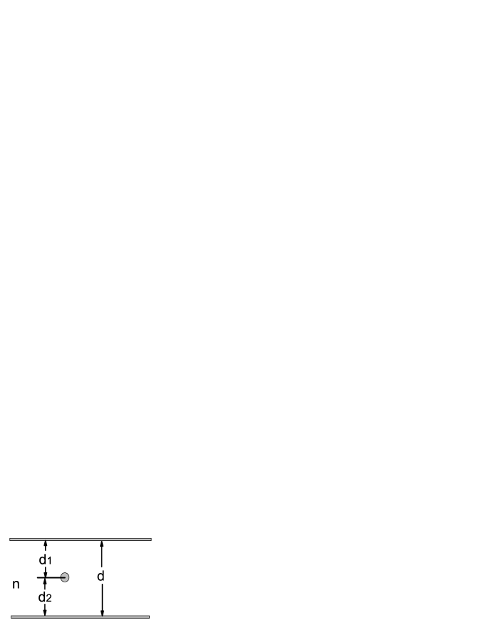
Figure 1: Schematic diagram for emitting atom in a medium with an arbitrary refractive index $n$ between two perfect parallel plane mirrors.

The schematic diagram of the system is shown in Fig. 1. An atom is placed between two perfect parallel plane mirrors, and a medium with refractive index $n$ fills up the space between the mirrors. Denote the distance between the two mirrors by $d$. We choose the coordinate system such that the origin is in the middle of the two mirrors and the $z$-axis is perpendicular to the mirrors. The emitting atom is placed at $z$, its distance from the upper (lower) mirror is denoted by $d_{1}$ and $d_{2}$. Using Fermi’s golden rule and following the approach developed for the case when the space between two mirrors is vacuum 9 ; 10 ; 11 ; 12 , the spontaneous emission rate for this system can be derived. When the transition dipole moment $\vec{d}_{12}$ is parallel to the mirror planes, the emission rate formula is

$$W(z)=W_{vac}\frac{3\pi c}{2d\omega_{0}}\sum_{j=1}^{M}(1+\frac{j^{2}\pi^{2}}{n^{2}k^{2}_{0}d^{2}})\sin^{2}(\frac{j\pi z}{d}-\frac{j\pi}{2}),$$ (1)

where $W_{vac}$ is the emission rate in vacuum without mirrors, $M$ is the greatest integer part of $nk_{0}d/\pi$ , $k_{0}=\omega_{0}/c$ is the wave number of the emitted light in vacuum, $z$ is the coordinate of the emitting atom. The derivation of formula (1) is given in Appendix A for completeness.

To investigate the multi-periodic oscillations in the spontaneous emission rate, we follow the approach for the dielectric slabs 2 and use $R=(d_{2}-d_{1})/(d_{2}+d_{1})$ to indicate the configuration of the system. We also use a variable $\alpha$ to indicate the system size relative to a standard one. We take the standard distance between the two mirrors as the wavelength of the emitted photon in vacuum, that is, $d^{0}=\lambda_{0}=2\pi/k_{0}$, then we have the relationship $z=\alpha Rd^{0}/2$ , $d_{1}=\alpha(1-R)d^{0}/2$ and $d_{2}=\alpha(1+R)d^{0}/2$. In order to compare with the spontaneous emission rate in dielectric slabs 2 , we also set the refractive index $n=1.49$ appropriate for the poly methyl methacrylate (PMMA) material between the two mirrors. In Fig. 2 we show the spontaneous emission rate as a function $\alpha$ for $R=0,1/3$, and $3/5$. In Fig. 2(a), $R=0$, the emitting atom is in the middle of the mirrors, the emission rate is like a saw-tooth; In Fig. 2(b), $R=1/3$, the distance between the emitting atom and the lower mirror is twice of the distance between the emitting atom and the upper mirror, some smaller tooth appeared; In Fig. 2(c), the emitting atom is even closer to the upper mirror, the distance between the emitting atom and the lower mirror is four times of the distance between the emitting atom and the upper mirror, finer tooth appeared. These figures can be compared with the more smooth emission rate in dielectric slabs 2 .

The oscillations in these figures are not obvious but can be extracted using modified Fourier transforms defined by

$$\tilde{W}(\gamma)=\int_{\alpha_{1}}^{\alpha_{2}}[W(\alpha)-W_{bg}]\alpha e^{i\alpha\gamma}d\alpha,$$ (2)

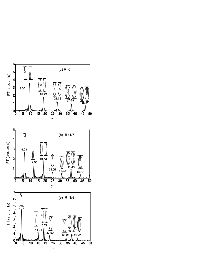
Figure 3: Fourier transforms of the spontaneous emission rate in Fig. 2 (solid lines) are compared with the analytical results (crosses) based on closed-orbits. Closed-orbits corresponding to the peaks are shown schematically in the inserts.

where $W_{bg}=nW_{vac}$ is the non-oscillating background emission rate in the medium without mirrors. In Eq.(2) $W(\alpha)$ represents the dependence of the emission rate as a function of the scaling variable $\alpha$ . Assuming $\gamma^{\prime}$ is the first peak position of the Fourier transform in the range $[\gamma_{min},\gamma_{max}]$, the integration range should satisfy $(\alpha_{2}-\alpha_{1})\geq 2\pi/\gamma^{\prime}$ and the step size $\Delta\alpha$ should satisfy $\Delta\alpha\leq 0.1\times 2\pi/\gamma_{max}$to ensure numerical accuracy. In our calculations, we took $\alpha_{1}=1$, $\alpha_{2}=16$, $\Delta\alpha=0.01$. The calculated Fourier transformations of the rates in Fig.2 as defined in Eq.(2) are presented as solid lines in Fig.3. The numerical value near each peak is the extracted peak position. There are five peaks in Fig. 3(a) when $R=0$, seven peaks in Fig. 3(b) when $R=1/3$, and seven peaks in Fig. 3(c) when $R=3/5$. Many more peaks are present in Fig.3 compared to the dielectric slab system 2 .

III The oscillations and closed-orbits

We now provide an explanation of the physical meaning for the peaks and give a quantitative description for the peak positions and peak heights. Over the last ten years, closed-orbit theory has been used successfully to understand the oscillations in the absorption spectra of atoms and negative ions in external fields 4 ; 5 ; 6 ; 7 . The oscillations in the absorption spectra correspond to electron closed-orbits, and they are interpreted as interferences between outgoing electron and returning electron. The similarity between the oscillations in the spontaneous emission rate and the oscillations in the absorption spectra has inspired the recent studies of the oscillations in the spontaneous emission near dielectric interfaces 2 ; 3 . The oscillations in the spontaneous emission rates correspond to closed-orbits of emitted photon and they are interpreted as interference effects between emitted photon going away from and returning to the atom following various closed-orbits. This view can be made more quantitative for the present system.

Consider the radiation damping of a dipole antenna 13 . The dipole moment is $\vec{d}e^{-i\omega_{0}t}$ , where $\omega_{0}$ is the frequency of oscillation. The radiation damping rate is $W_{d}=P/U$ where $P$ is the average radiation power of the antenna, $U$ is the energy of the antenna. The radiation damping rate can be written as 13

$$W=\frac{\omega_{0}}{2U}{\rm{Im}}(\vec{d}^{*}\cdot\vec{E})=\frac{\omega_{0}}{2U}[{\rm{Im}}(\vec{d}^{*}\cdot\vec{E}_{0})+{\rm{Im}}(\vec{d}^{*}\cdot\vec{E}_{ret})],$$ (3)

where we have decomposed the electric field $\vec{E}$ at the position of dipole antenna into a direct part $\vec{E}_{0}$ and a returning part $\vec{E}_{ret}$. This step for the electric field is similar to a step for the electron wave function in the derivation of closed-orbit theory 4 ; 5 ; 6 . Using $\vec{r}$ to denote the vector of a point relative to the dipole position, the direct electric field is

$$\vec{E}_{0}=\frac{dk^{3}}{4\pi\epsilon}\{(\hat{r}\times\hat{d})\times\hat{r}(\frac{1}{kr})+[\hat{d}-3\hat{r}(\hat{r}\cdot\hat{d})]\times(\frac{i}{(kr)^{2}}-\frac{1}{(kr)^{3}})\}e^{i(kr-\omega_{0}t)}.$$ (4)

The returning electric field $\vec{E}_{ret}$ depends on the environments or the cavity. If the dipole antenna is at distance $l$ from the mirror and is parallel to the mirror, $\vec{E}_{ret}$ can be calculated exactly using an imaging method 13 . The returning field at the position of the antenna is

$$\vec{E}_{ret}=-\frac{dk^{3}}{4\pi\epsilon}\hat{d}(\frac{1}{2kl}+\frac{i}{(2kl)^{2}}-\frac{1}{(2kl)^{3}})e^{i(2kl-\omega_{0}t)},$$ (5)

where $\hat{d}$ is a unit vector in the dipole direction. The damping rate for a dipole antenna in a medium with an arbitrary refractive index $n$ near one mirror and parallel to the mirror plane can be evaluated as

$$W_{d}=W_{0}-\frac{3}{2}W_{0}[\frac{\sin(2nk_{0}l)}{2nk_{0}l}+\frac{\cos(2nk_{0}l)}{(2nk_{0}l)^{2}}-\frac{\sin(2nk_{0}l)}{(2nk_{0}l)^{2}}],$$ (6)

where $W_{0}=\frac{2}{3}\frac{d^{2}k^{3}}{4\pi\epsilon}\frac{\omega_{0}}{2U}$ . Eq.(6) is a generalization of the vacuum case $n=1$ 13 . When the distance between the dipole antenna and the mirror is greater than half of a wavelength, the last two terms in the square bracket are small enough and can be neglected. The semi-classical approximation for the damping rate of a dipole near one mirror becomes

$$W_{d}=W_{0}-\frac{3}{2}W_{0}\frac{\sin(S)}{S},$$ (7)

where $S=2nk_{0}l$ is the action of the emitted photon going from the atom to the mirror and back to the atom. This path is a closed-orbit. For a dipole antenna in a medium with an arbitrary refractive index $n$ between two mirrors, the semi-classical formula for the damping rate can be generalized to

$$W_{d}=W_{0}-\frac{3}{2}W_{0}\sum_{j}\frac{1}{S_{j}}\sin(S_{j}+\phi_{j}),$$ (8)

where $S_{j}=nk_{0}L_{j}$ is the action of the $j$-th emitted photon closed-orbit, $L_{j}$ is the corresponding geometric length of the orbit, $\phi_{j}=-m_{j}\pi$ is a phase correction, $m_{j}$ counts the number of reflections by the two mirrors. We identify $W_{d}$ and $W_{0}$ in Eq.(8) with the spontaneous rate $W$ and $W_{bg}$ for the spontaneous emission rate formula in Eq.(1). Eq.(8) is quite similar to the formula in closed-orbit theory. The peak positions in the Fourier transform of Eq.(2) are given by the action $S_{j}^{0}$ of emitted photon closed-orbits with corresponding peak height proportional to $g/L_{j}^{0}$, where $L_{j}^{0}$ is the length of the closed-orbit, $g$ is a degeneracy factor counting the number of closed-orbit having the same length. Both $S_{j}^{0}$ and $L_{j}^{0}$ are evaluated for the standard system size corresponding to $\alpha=1$. We have the scaling relationship $L_{j}(\alpha)=\alpha L_{j}^{0}$ and $S_{j}(\alpha)=\alpha S_{j}^{0}$.

The above predictions for the peak positions and peak heights in the Fourier transforms (FT) are marked as crosses in Fig.3. We fixed the constant $h$ using one peak height and then calculated other peak height using $hg/L_{j}^{0}$. For all the peaks in Fig.3, the predications from Eq.(8) for both the peak positions and the peak heights agree well with the numerically extracted values from the rate formula in Eq.(1). For the case $R=0$, there are five peaks. Each peak corresponds to two closed-orbits. The structures of the closed-orbits are shown as inserts next to the peaks in Fig. 3(a). The first peak in Fig. 3(a) corresponds to two closed-orbits going away from and returning to the emitting atom after being reflected back by the upper or the lower mirror once. These two closed-orbits have the same action $S_{1,2}^{2}=2\pi n=9.36$; the third (fourth) closed-orbit leaves from and returns to the emitting atom after reflected by both mirrors. The action for the third or fourth closed-orbit is $S_{3,4}^{0}=4\pi n=18.72$. The fifth (sixth) closed-orbit is reflected three times by the mirrors. Their actions are $S^{0}_{5,6}=6\pi n=28.09$. Similar discussions can be made for other peaks in Fig.3(a). The double degeneracy for some of the peaks can be removed when the emitting atom is away from the middle point. For example, when $R=1/3$, the first peak at $9.35$ in Fig.3(a) splits to two peaks at $6.23$ and at $12.50$ in Fig.3(b). The peak at $6.23$ corresponds to the closed-orbit produced by the reflection of the upper mirror closer to the emitting atom, while the peak at $12.50$ is produced by the reflection of the lower mirror that is further away from the emitting atom. In Table I, we compare the extracted values and the theoretical predictions for the peak positions and peak heights in Fig.3. They agree very well.

Table 1: Peak positions and peak heights extracted from Eq.(1) using Fourier transform (FT) are compared with the analytic predications of Eq.(8).

		Peak position		Peak height
	peak index	FT	Eq. (8)	FT	Eq. (8)
	$1^{st}$	9.35	9.36	3.5987	3.5993
	$2^{nd}$	18.72	18.72	1.8175	1.7977
R=0	$3^{rd}$	28.08	28.09	1.1957	1.1984
	$4^{th}$	37.45	37.45	0.90616	0.8986
	$5^{th}$	46.81	46.81	0.72541	0.7189
	$1^{st}$	6.23	6.24	2.6839	2.7009
	$2^{nd}$	12.50	12.48	1.3692	1.3461
	$3^{rd}$	18.72	18.72	1.8102	1.7977
R=1/3	$4^{th}$	24.95	24.97	0.65365	0.6744
	$5^{th}$	31.22	31.21	0.55291	0.5390
	$6^{th}$	37.45	37.45	0.90279	0.8986
	$7^{th}$	43.67	43.69	0.37436	0.3853
	$1^{st}$	3.73	3.74	4.5112	4.5112
	$2^{nd}$	14.94	14.98	1.1261	1.1263
	$3^{rd}$	18.72	18.72	1.7920	1.7977
R=3/5	$4^{th}$	22.50	22.47	0.7551	0.7479
	$5^{th}$	33.66	33.70	0.50151	0.4999
	$6^{th}$	37.44	37.45	0.8917	0.8989
	$7^{th}$	41.22	41.19	0.40507	0.4082

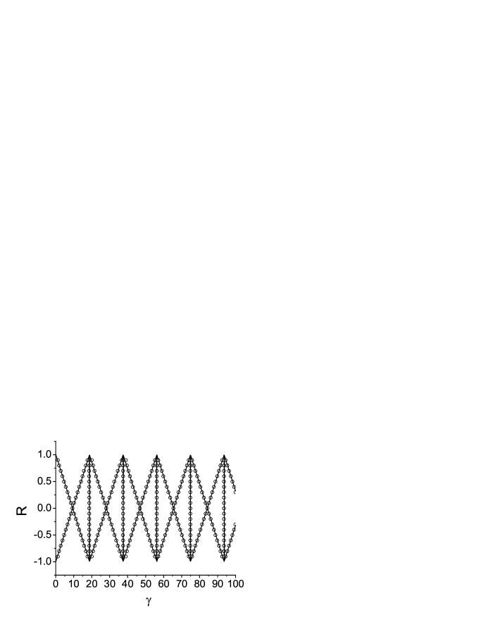
Figure 4: Peak positions extracted from Eq.(1) using Fourier transforms (circles) are compared with the predictions of closed-orbits in Eq.(8) as a function of $R$. 16 visible peaks can be clearly identified for most of $R$ in this range.

In Fig.4 we compare the peak positions extracted from Eq.(1) using Fourier transform (circles) with the analytic predication (solid lines) as a function of $R$. 16 peaks can be clearly identified in the specified range. The numerical and analytic results for the peak positions are in excellent agreement. The large number of peaks identified for this system is in contrast with the previous systems with dielectric interfaces 2 ; 3 where only one or three peaks were clearly identified. The difference in the number of identifiable peaks in these systems can be explained by the difference between a dielectric interface and a mirror in reflecting emitted photon waves. In deriving Eq.(8), it is clear that the peak height is proportional to the wave amplitude when it returns to the position of the dipole. For a closed-orbit $j$, it is being reflected $m_{j}$ times by mirrors or dielectric interfaces. A mirror reflects better than a dielectric interface, consequently the returning wave corresponding to the same closed-orbit is stronger in a mirror system and many more peaks can be identified.

Eq.(8) is a sum over closed-orbits. In Fig.5 we show how the sum over closed-orbits converges to the rate formula in Eq.(1). Fig.5(a) demonstrates that 4 closed-orbits already gives a rather accurate representation of the rate that requires a large number of terms in Eq.(1). When the closed-orbits are increased to 16 as in Fig.5(b), the oscillations are greatly reduced. When we use 100 closed-orbits in Eq.(8) as shown in Fig.5(c), the sum over closed-orbits in Eq.(8) accurately represents the golden rule rate in Eq.(1).

IV Conclusions

In conclusions, we have studied the oscillations in the spontaneous emission of an atom in a medium with an arbitrary refractive index $n$ between two large perfect plane mirrors. We have compared the golden rule formula in Eq.(1) and the summation formula over closed-orbits in Eq.(8). The oscillations in the golden rule formula can be extracted when the system scale is varied while the system configuration is fixed. The extracted peak positions and peak heights agree well with Eq.(8) based on closed-orbits of emitted photon going away and returning to the atom. The oscillations in the spontaneous emission rate are quite similar to the oscillations in the absorption spectra described by closed-orbit theory 4 ; 5 ; 6 ; 7 . For other systems, in principle, we can follow the propagation of the electric field along various closed-orbits until they are back to the emitting atom to calculate the radiation damping rate using Eq.(3). This would give us a formula of the rate in terms of closed-orbits. Our study suggests the rate formula based on Fermi’s golden rule and the rate formula involving a sum over closed-orbits provide complementary perspectives on spontaneous emission process.

ACKNOWLEDGMENTS

This work was supported by NSFC grant No. 90403028.

Appendix A derivation of formula in Eq.(1)

The emitting rate is given by Feimi’s golden rule 13 . The transition rate is

$$W=\frac{2\pi}{\hbar^{2}}\sum_{\alpha}|\langle e,0|-\frac{q}{m}\vec{p}\cdot\vec{A}(\vec{x}^{\prime})|q,1_{\alpha}\rangle|^{2}\delta(\omega_{\alpha}-\omega_{eq})$$ (9)

where $|e,0\rangle$ is the system initial state, in which the atom is excited and there is no photon in the field; $|q,1_{\alpha}\rangle$ is the system final state, in which the atom is in final state and there is one photon with frequency $\omega_{\alpha}$ in the field; $q$ is the charge of the electron of the atom, and $m$ is the mass of the electron; $\vec{p}$ is the momentum of the electron, and $\vec{A}(\vec{x}^{\prime})$ is the quantized transverse vector potential, and $\vec{x}^{\prime}$ is the position of atom; $\omega_{qe}$ is the frequency $(E_{e}-E_{q})/\hbar$. $\vec{A}(\vec{x})$ can be write as

$$\vec{A}(\vec{x})=\sum_{\alpha}\sqrt{\frac{\hbar}{2n^{2}\epsilon_{0}\omega_{\alpha}}}[\vec{A}_{\alpha}(\vec{x})a_{\alpha}+\vec{A}_{\alpha}^{*}(\vec{x})a_{\alpha}^{\dagger}]$$ (10)

where

$$\bigtriangledown^{2}\vec{A}_{\alpha}(\vec{x})+k^{2}_{\alpha}\vec{A}_{\alpha}(\vec{x})=0,~{}~{}k_{\alpha}^{2}=\frac{\omega_{\alpha}^{2}n^{2}}{c^{2}},$$ (11)

$$\bigtriangledown\vec{A}_{\alpha}(\vec{x})=0,$$ (12)

$n$ is the refractive index of the dielectric medium, and the mode function are chosen to form an orthonormal set:

$$\int d^{3}x\vec{A}_{\alpha}^{*}(\vec{x})\cdot\vec{A}_{\beta}(\vec{x})=\delta_{\alpha\beta}.$$ (13)

Using Eqs. (9) and (10) we find

$$W=\frac{2\pi}{\hbar^{2}}\sum_{\alpha}\frac{q^{2}\hbar}{2m^{2}\epsilon_{0}n^{2}\omega_{\alpha}}|\vec{p}_{eq}\cdot\vec{A}_{\alpha}(\vec{x}^{\prime})|^{2}\delta(\omega_{\alpha}-\omega_{eq})$$ (14)

where $\vec{p}_{eq}=\langle e|\vec{p}|q\rangle$ . Using $q\vec{p}_{eq}=-im\omega_{eq}\vec{d}_{eq}$ and Eq. (A6) we get

$$W=\frac{\pi\omega^{2}_{eq}}{\hbar\epsilon_{0}n^{2}}\sum_{\alpha}\frac{1}{\omega_{\alpha}}|\vec{d}_{eq}\cdot\vec{A}_{\alpha}(\vec{x}^{\prime})|^{2}\delta(\omega_{\alpha}-\omega_{eq})$$ (15)

where $\vec{d}_{eq}$ is the electric dipole matrix element.

Consider our boundary conditions: the mirrors are in $z=-d/2$ and $z=d/2$ , and therefore the mode function must vanish at this two planes. According to Ref. 10 we write the mode functions as

$$A_{\vec{k}_{1}}(\vec{x})=(\frac{2}{V})^{1/2}(\hat{k}_{\|}\times\hat{z})\sin k_{3}(z-\frac{d}{2})e^{i\vec{k}_{\|}\cdot\vec{x}}$$ (16)

$$A_{\vec{k}_{2}}(\vec{x})=\frac{1}{k}(\frac{2}{V})^{1/2}[k_{\|}\hat{z}\cos k_{3}(z-\frac{d}{2})-ik_{3}\hat{k}_{\|}\sin k_{3}(z-\frac{d}{2})]e^{i\vec{k}_{\|}\cdot\vec{x}}$$ (17)

where $\vec{k}_{\|}$ is the parallel component of $\vec{k}$ , and $\vec{k}_{3}=j\frac{\pi}{d},(j=1.2.\cdots)$ . We consider $\vec{d}_{eq}$ is parallel the mirror and set $\phi$ as the angle between $\vec{k}_{\|}$ and $\vec{d}_{eq}$. Then we get

$$|\vec{A}_{\alpha}(\vec{x})\cdot\vec{d}_{eq}|^{2} = \frac{2}{V}[|(\hat{k}_{\|}\times\hat{z})\cdot\vec{d}_{eq}|^{2}\sin^{2}k_{3}(z-\frac{d}{2})+\frac{k_{3}^{2}}{k_{\alpha}^{2}}|\hat{k}_{\|}\cdot\vec{d}_{eq}|^{2}\sin^{2}k_{3}(z-\frac{d}{2})]$$ (18)

$$= \frac{2|\vec{d}_{eq}|^{2}}{V}[(\sin^{2}\phi+\frac{k_{3}^{2}}{k_{\alpha}^{2}}\cos^{2}\phi)\sin^{2}k_{3}(z-\frac{d}{2})]$$ (19)

Using Eq. (15) and (19), we get

$$W = \frac{\pi\omega^{2}_{eq}}{\hbar\epsilon_{0}n^{2}}\sum_{k_{3}}\frac{L^{2}}{4\pi^{2}}\int_{0}^{\infty}dk_{\|}k_{\|}\int_{0}^{2\pi}d\phi\frac{2|\vec{d}_{eq}|^{2}}{V}[(\sin^{2}\phi+\frac{k_{3}^{2}}{k_{\alpha}^{2}}\cos^{2}\phi)$$

$$\times\sin^{2}k_{3}(z-\frac{d}{2})]\frac{1}{\omega_{\alpha}}\delta(\omega_{\alpha}-\omega_{eq})$$ (20)

$$= \frac{\pi\omega^{2}_{eq}}{\hbar\epsilon_{0}n^{2}}\frac{L^{2}}{4\pi^{2}}\frac{2|\vec{d}_{eq}|^{2}}{V}\sum_{k_{3}}\int_{0}^{\infty}dk_{\|}k_{\|}\pi(1+\frac{k_{3}^{2}}{k^{2}_{\alpha}})$$

$$\times\sin^{2}k_{3}(z-\frac{d}{2})\frac{n}{ck}\frac{n^{2}k_{0}}{ck_{\|}}\delta(k_{\|}-\sqrt{n^{2}k_{0}^{2}-k_{3}^{2}})$$ (21)

$$= \frac{\pi\omega^{2}_{eq}}{\hbar\epsilon_{0}n^{2}}\frac{L^{2}}{4\pi^{2}}\frac{2|\vec{d}_{eq}|^{2}}{V}\sum_{k_{3}}\pi(1+\frac{k_{3}^{2}}{n^{2}k_{0}^{2}-k_{3}^{2}+k_{3}^{2}})\sin^{2}k_{3}(z-\frac{d}{2})\frac{n}{ck}\frac{n^{2}k_{0}}{c}$$ (22)

$$= \frac{\pi\omega^{2}_{eq}}{\hbar\epsilon_{0}n^{2}}\frac{L^{2}}{4\pi^{2}}\frac{2|\vec{d}_{eq}|^{2}}{V}\frac{n}{ck}\frac{n^{2}k_{0}}{c}\pi\sum_{j}(1+\frac{j^{2}\pi^{2}}{d^{2}n^{2}k_{0}^{2}})\sin^{2}(\frac{j\pi z}{d}-\frac{j\pi}{2})$$ (23)

$$= W_{vac}\frac{3\pi}{2k_{0}d}\sum_{j}^{M}(1+\frac{j^{2}\pi^{2}}{d^{2}n^{2}k_{0}^{2}})\sin^{2}(\frac{j\pi z}{d}-\frac{j\pi}{2})$$ (24)

where $W_{vac}=\frac{\omega_{eq}^{3}|\vec{d}_{eq}|^{2}}{3\hbar\epsilon_{0}\pi c^{3}}$ is the emission rate in vacuum.

Figure 2: Spontaneous emission rate (in unit of rate in vacuum) as a function of $\alpha=d/d^{0}$ , where $d^{0}$ is the emitted photon wavelength in vacuum. The three cases in (a), (b), and (c) correspond to $R=(d_{2}-d_{1})/(d_{2}+d_{1})=0$, $1/3$, and $3/5$, respectively.

Figure 5: The spontaneous emission rate in Eq.(1) (solid lines) and the representation using a finite number of closed-orbits in Eq.(8) (dotted lines). (a) $4$ closed-orbits; (b) $16$ closed-orbits; (c) $100$ closed-orbits.

References

- (1) R. G. Hulet, E. S. Hilfer, and D. Kleppner, Phys. Rev. Lett. 55, 2137 (1985); D. Kleppner, Phys. Rev. Lett. 47, 233 (1981); E. M. Purcell, Phys. Rev. 69, 37 (1946).
- (2) M. L. Du, Fu-He Wang, Yan-Ping Jin, Yun-Song Zhou, Xue-Hua Wang, and Ben-Yuan Gu Phys. Rev. A71, 065401 (2005)
- (3) F.-H. Wang, Y.-P. Jin, B.-Y. Gu, Y.-S. Zhou, X.-H. Wang, and M. L. Du, Phys. Rev. A71, 044901 (2005).
- (4) M. L. Du and J. B. Delos, Phys. Rev. Lett. 58, 1731 (1987).
- (5) M. L. Du and J. B. Delos, Phys. Rev. A38, 1896 (1988).
- (6) M. L. Du and J. B. Delos, Phys. Rev. A38, 1913 (1988).
- (7) D. Kleppner and J. B. Delos, Found. Phys. 31, 5932001, and references therein.
- (8) M. L. Du, Phys. Rev. A70, 055402 (2004); M. L. Du and J. B. Delos, Phys. Rev. A38, 5609 (1988);
- (9) P. W. Milonni, The Quantum Vacuum : An Introduction to Quantum Electrodynamics (Academic Press, London, 1994).
- (10) P. W. Milonni and P. L. Knight, Optics Comm. 9, 119 (1973).
- (11) G. Barton, Proc. Roy. Soc. Lond. A320, 251 (1970).
- (12) Michael R. Philpott, Chem. Phys. Lett. 19, 435 (1973).
- (13) E. A. Hinds, Advances in atomic, molecular, and optical physics. Supplement 2, (Academic Press, San Diego, 1990)