Phase vortices from a Young’s three-pinhole interferometer

Abstract

An analysis is presented of the phase vortices generated in the far field, by an arbitrary arrangement of three monochromatic point sources of complex spherical waves. In contrast with the case of three interfering plane waves, in which an infinitely-extended vortex lattice is generated, the spherical sources generate a finite number of phase vortices. Analytical expressions for the vortex core locations are developed and shown to have a convenient representation in a discrete parameter space. Our analysis may be mapped onto the case of a coherently-illuminated Young’s interferometer, in which the screen is punctured by three rather than two pinholes.

I Introduction

In a seminal paper, Dirac (1931) considered vortical screw-type dislocations in the phase of complex wavefields, noting the one-dimensional nature of the associated vortex cores (nodal lines) in three dimensions (3D). Such phase vortices exist in a variety of linear and non-linear physical systems that may be described via complex fields, including the angular-momentum eigenstates of the hydrogen atom (Messiah, 1961a), the Meissner state of type-II superconductors (Abrikosov, 1957; Tilley and Tilley, 1990), vortex states of superfluids (Feynman, 1955; Pismen, 1999) and Bose–Einstein condensates (Pitaevskii and Stringari, 2003), optical vortex solitons (Desyatnikov et al., 2005), propagating electron wavefunctions diffracting through crystalline slabs (Allen et al., 2001), Gaussian random wavefields (Berry, 1978) and optical speckle fields (Freund et al., 1993).

In continuous complex scalar fields, to which the considerations of the present paper are restricted, vortical behavior is manifest as screw-type dislocations in the field’s multi-valued surfaces of constant phase (Riess, 1970; Nye and Berry, 1974; Hirschfelder et al., 1974). More precisely, consider a stationary-state, complex spatial wavefunction or order-parameter field $\Psi(\boldsymbol{\mathrm{r}})=A(\boldsymbol{\mathrm{r}})\exp\left[i\chi(\boldsymbol{\mathrm{r}})\right]$. Here, $A(\boldsymbol{\mathrm{r}})$ is the non-negative real amplitude, $\chi(\boldsymbol{\mathrm{r}})$ is the phase, and $\boldsymbol{\mathrm{r}}=(x,y,z)$ is a position vector in 3D. Note that harmonic time dependence on angular frequency $\omega$ and time $t$, via the usual multiplicative factor of $\exp(-i\omega t)$, is suppressed throughout. To determine whether a phase vortex exists at a point $p$ in a plane $\Pi$ over which $\Psi(\boldsymbol{\mathrm{r}})$ is defined, a line integral of the phase gradient is evaluated along a smooth infinitesimally-small path $\Gamma$ that encircles $p$. This path is assumed to have a winding number of unity with respect to $p$, and to be such that the modulus of $\Psi(\boldsymbol{\mathrm{r}})$ is strictly positive at each point on $\Gamma$. One may then write the following expression for the “circulation” of the field over $\Gamma$ (see, e.g., Nye (1999)):

$$\oint_{\Gamma}d\chi=\oint_{\Gamma}\nabla\chi\cdot\boldsymbol{\mathrm{t}}\ ds=2\pi n.$$ (1)

Here, $\boldsymbol{\mathrm{t}}$ is a unit tangent vector to $\Gamma$, $ds$ is an infinitesimal line element along $\Gamma$, and $n$ is an integer corresponding to the number of phase windings about $p$. Any non-zero $n$ indicates the presence of a vortex core threading the path $\Gamma$, with the non-zero value for $n$ being referred to as its topological charge. The sign of this charge distinguishes between a vortex ($+$) and an anti-vortex ($-$).

In an optical setting, a common way to generate such phase vortices is to pass coherent laser or soft X-rays through a spiral phase plate or forked transmission diffraction grating (Heckenberg et al., 1992a, b; He et al., 1995; Peele and Nugent, 2003; Okamoto and Sasada, 2005; Kotlyar et al., 2006). Kim et al. (1997) generated optical vortices with a curved glass plate as an alternative to the spiral phase plate. Another means for generating fields with specified vortical phase is a dynamically computer-controlled, holographic system (Kishima et al., 2006). Other means for creating optical phase vortices in coherent light include the use of spatial light modulators (Curtis and Grier, 2003), the use of aberrated lenses to create vortices in a distorted focal volume (Boivin et al., 1967), and diffraction from random phase screens (Berry, 1978).

As an alternative approach, one can forego the use of diffractive or refractive optical elements, seeking instead to create phase vortices by the superposition of a small number of non-vortical fields. For example, Nicholls and Nye (1987) showed that one can generate a lattice of vortices by interfering three plane waves. Later, Masajada and Dubik (2001) showed that this is a minimum requirement and reformulated the analysis in terms of phasors.

Here we generalize this idea, by considering the formation of phase vortices via the superposition of three outgoing spherical waves, generated by three distinct monochromatic equal-energy point sources. We see that the resulting system of nodal lines (vortex cores) exhibits a rich geometry, by developing approximate analytical expressions for the far-field behaviour of this nodal-line network. The three-dimensional space, into which the sources radiate, is foliated using a family of observation planes that are parallel to the plane containing the three point sources. When one observes the wavefield over any such foliating plane, a 2D pattern of point vortices may be seen, the cores of which coincide with the points at which a nodal line punctures the plane.

Interestingly, the problem of three interfering spherical waves may be mapped onto a Young-type experiment, in which a black screen with three small pinholes is coherently illuminated by a propagating complex scalar field. Note that this identification is only possible when one is both sufficiently far from the screen and sufficiently close to the optic axis, in which case the radiation transmitted by each of the pinholes is approximately spherical.

We close this introduction with a brief outline of the remainder of the paper: We begin by reviewing the manner in which the superposition of three plane waves may be used to generate an infinite lattice of phase vortices. The generalization of this idea, to the superposition of three outgoing spherical waves, is then given. We describe the application of a phasor approach to the spherical-wave arrangement, applying this in the far-field region asymptotically far from the sources. Approximate analytical expressions are derived for the vortex locations. A representation in terms of a certain parameter space arises, allowing estimates of the number of vortices and description of a natural coordinate system for the vortices at the intersections of a certain family of hyperbolas. A specific case of collinear sources is explored in detail. We then show how the theory, which has been derived for spherical point sources, may be mapped onto the case of a Young’s interferometer in which the illuminated screen contains three rather than two pinholes.

II Phase vortices from the interference of three plane waves

Consider the following superposition of three planar spatial wavefunctions:

$$\Psi(\boldsymbol{\mathrm{r}})=\sum_{j=1}^{3}A_{j}\exp\left[i\left(\boldsymbol{\mathrm{k}}_{j}\cdot\boldsymbol{\mathrm{r}}+\phi_{j}\right)\right],$$ (2)

where the non-negative real constants $A_{j}$ denote the amplitude of the $j$th wave, $\boldsymbol{\mathrm{k}}_{j}$ are wavevectors corresponding to the same de Broglie wavelength $\lambda_{0}=2\pi/|\boldsymbol{\mathrm{k}}_{j}|$, and $\phi_{j}$ are global phase factors. Notwithstanding the fact that the constituent plane waves do not have a vortical character, the above superposition may yield a regular lattice of phase vortices and anti-vortices (Nicholls and Nye, 1987; Masajada and Dubik, 2001).

A numerical example of this phenomenon is given in Fig. 1, corresponding to the parameters $A_{1}=A_{2}=A_{3}=1$ and $\phi_{1}=\phi_{2}=\phi_{3}=0$, with all fields being evaluated over the plane $z=0$. This example illustrates the three interfering plane waves giving rise to an infinitely extended lattice of straight, parallel nodal lines (vortex cores). These nodal lines intersect the plane $z=0$, to give the location of the point vortices that are visible as screw dislocations in the phase map of Fig. 1(d). The locations of these point vortices coincide with both (i) the intersections of the zero contours in Fig. 1(b), and (ii) the points at which $|\Psi|=0$ in the amplitude plot of Fig. 1(c). Indeed, continuity of the wavefunction implies that the probability density vanishes at each vortex core, since these are branch points at which the phase ceases to be differentiable. The topological charge $n$ of each of these point defects is seen to be equal to $\pm 1$, as the phase increases by $\pm 2\pi$ as one traverses a circuit that encloses a given vortex core. In this context, we note that higher-charge vortices are unstable with respect to perturbation (Freund, 1999), which is why they are not observed in the present setting.

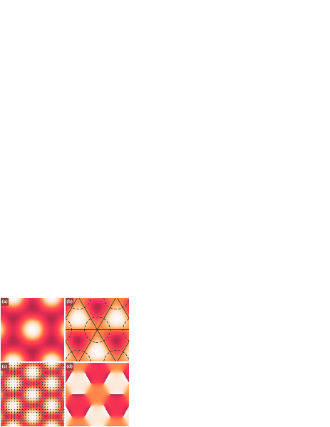
Figure 1: (Color online) Interference of three plane waves giving rise to an infinite, regular vortex lattice [see Eq. (2)]. Here the wavevectors are oriented symmetrically with respect to the $z$ axis, with $\boldsymbol{\mathrm{k}}_{1}=(\sqrt{3},-1,10),\boldsymbol{\mathrm{k}}_{2}=(-\sqrt{3},-1,10)$ and $\boldsymbol{\mathrm{k}}_{3}=(0,2,10)$. The real (a) and imaginary (b) parts, amplitude (c), and phase (d) of the wavefunction $\Psi(x,y,z=0)$ are shown. In (b), zero contours of the real (dashed lines) and imaginary (solid lines) parts are overlaid. In (c) is overlaid the vector field of the probability current density, which is seen to rotate counter-clockwise around vortices and clockwise around anti-vortices. In (d), vortices are visible as the ends of branch cuts indicated by dark to light ($-\pi\rightarrow\pi$) steps. Values in (a-c) are represented by linear levels from dark to light (minimum to maximum).

III Phase vortices from the interference of three spherical waves

Given that the superposition of three complex plane-wave spatial wavefunctions may lead to phase vortices (Nicholls and Nye, 1987; Masajada and Dubik, 2001), it is natural to enquire whether the superposition of three outgoing spherical waves may not also lead to phase vortices. This latter case is investigated here.

III.1 Extending the plane-wave case to spherical waves

The complex spatial wavefunction $\Psi_{j}(\boldsymbol{\mathrm{r}})$, due to a point source at position $\boldsymbol{\mathrm{r}}_{j}$ that is radiating outgoing spherical waves in vacuo, is given by

$$\begin{split}\Psi_{j}(\boldsymbol{\mathrm{r}})&=\frac{A_{j}}{|\boldsymbol{\mathrm{r}}-\boldsymbol{\mathrm{r}}_{j}|}\exp\left[i\left(k|\boldsymbol{\mathrm{r}}-\boldsymbol{\mathrm{r}}_{j}|+\phi_{j}\right)\right]\\ &\equiv\frac{A_{j}}{|\boldsymbol{\mathrm{r}}-\boldsymbol{\mathrm{r}}_{j}|}\exp\left(i\chi\right),\end{split}$$ (3)

where $k\equiv 2\pi/\lambda_{0}$. For all $\boldsymbol{\mathrm{r}}\neq\boldsymbol{\mathrm{r}}_{j}$, such spherical waves obey a variety of linear partial differential equations, including: (i) the time-independent free-space Schrödinger equation for non-relativistic spinless particles, (ii) the time-independent free-space Klein-Gordon equation for relativistic spinless particles, and (iii) the free-space Helmholtz equation for monochromatic complex scalar electromagnetic waves. As such, the following discussions are applicable to all of these physical systems.

Now consider an assembly of three point sources, all of which have the same wave-number $k$. Without loss of generality we may consider these sources to occupy the same plane $z=0$, with source locations $\boldsymbol{\mathrm{r}}_{j}\equiv(x_{j},y_{j},0)$, where $j=1,2,3$. The resulting spatial wavefunction $\Psi(\boldsymbol{\mathrm{r}})$ may thus be written as

$$\Psi(\boldsymbol{\mathrm{r}})=\sum_{j=1}^{3}\frac{A_{j}}{|\boldsymbol{\mathrm{r}}-\boldsymbol{\mathrm{r}}_{j}|}\exp\left[i\left(k_{j}|\boldsymbol{\mathrm{r}}-\boldsymbol{\mathrm{r}}_{j}|+\phi_{j}\right)\right],$$ (4)

where $|\boldsymbol{\mathrm{r}}-\boldsymbol{\mathrm{r}}_{j}|\equiv\sqrt{(x-x_{j})^{2}+(y-y_{j})^{2}+z^{2}}$ is the distance from the $j{\rm th}$ source to a given observation point $\boldsymbol{\mathrm{r}}$.

Referring to Fig. 2, we label both the $j$th source and its distance from the coordinate origin by the same symbol $r_{j}$.

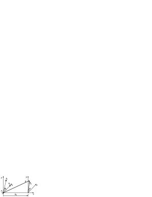
Figure 2: Coordinate system. The point sources $r_{1},r_{2}$, and $r_{3}$ lie in the plane $z=0$. The position vector $\boldsymbol{\mathrm{r}}$ is to a point with cylindrical-polar coordinates $(r_{\perp},\theta,z_{0})$.

The position vector $\boldsymbol{\mathrm{r}}$ and its perpendicular component $\boldsymbol{\mathrm{r}}_{\perp}$ have lengths $r\equiv|\boldsymbol{\mathrm{r}}|$ and $r_{\perp}\equiv|\boldsymbol{\mathrm{r}}_{\perp}|$, respectively.

To determine the location of the vortices which result from the superposition of the three spherical waves, we utilize the fact that vortex cores lie at points of zero amplitude. Given that the problem is restricted to two degrees of freedom, due to the complex wavefield representation, a geometric phasor diagram can be constructed with one phasor for each wave component in Eq. (4): see Fig. 3. We follow the phasor approach of Masajada and Dubik (2001) (see also (Paganin, 2006)).

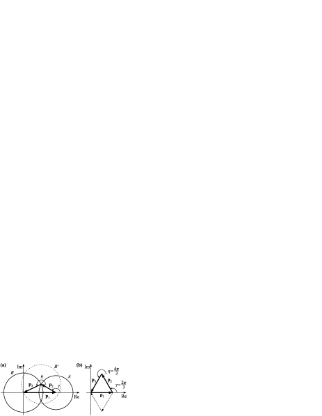
Figure 3: Phasor diagram from which vortex solution conditions are established (Masajada and Dubik, 2001). Three phasors $\boldsymbol{\mathrm{p}}_{1},\boldsymbol{\mathrm{p}}_{2},\boldsymbol{\mathrm{p}}_{3}$ — which respectively correspond to the three terms on the right side of Eq. (4), at a given point $\boldsymbol{\mathrm{r}}$ on a nodal line — form a closed triangle corresponding to a resultant zero amplitude. Two angles $\gamma$ and $\eta$ arise in the construction, as indicated. (a) In the case of arbitrary amplitudes for $\boldsymbol{\mathrm{p}}_{1}$, $\boldsymbol{\mathrm{p}}_{2}$ and $\boldsymbol{\mathrm{p}}_{3}$, the tip of $\boldsymbol{\mathrm{p}}_{2}$ is constrained to lie on circle $A$ of radius $|\boldsymbol{\mathrm{p}}_{2}|$, with the tail of $\boldsymbol{\mathrm{p}}_{3}$ being constrained to lie on circle $B$ of radius $|\boldsymbol{\mathrm{p}}_{3}|$. (b) For equal amplitudes $|\boldsymbol{\mathrm{p}}_{1}|=|\boldsymbol{\mathrm{p}}_{2}|=|\boldsymbol{\mathrm{p}}_{3}|$ an equilateral triangle is formed. The dashed construction represents another of the six equivalent alternatives formed by permutating the phasor order.

At any point coinciding with a vortex core, the phasor components must sum to zero when placed tip to tail. Note that if the source amplitudes differ sufficiently, it is possible that no closed triangle of phasors may be formed, i.e., circles $A$ and $B$ in Fig. 3 cannot intersect if $|\boldsymbol{\mathrm{p}}_{1}|>|\boldsymbol{\mathrm{p}}_{2}|+|\boldsymbol{\mathrm{p}}_{3}|$. In this case, no vortices will be produced.

Consider a given point $\boldsymbol{\mathrm{r}}$ in space, corresponding to the special case of Eq. (4) where $A_{1}=A_{2}=A_{3}=1$. Let $\boldsymbol{\mathrm{p}}_{1},\boldsymbol{\mathrm{p}}_{2},\boldsymbol{\mathrm{p}}_{3}$ denote the three complex terms that are summed on the right side of this equation. These three numbers are represented as phasors in Fig. 3. Here, we set $\phi_{1}=0$, which implies no loss of generality, since the invariance of the equations of motion under a shift in the origin of time implies global phase factors to have no physical meaning. The circle $B\,^{\prime}$ represents the possible orientations of $\boldsymbol{\mathrm{p}}_{3}$, constrained by the tip of $\boldsymbol{\mathrm{p}}_{2}$. The zero sum condition is easier to construct if $\boldsymbol{\mathrm{p}}_{3}$ is flipped and the circle $B$ drawn constrained by the tail of $\boldsymbol{\mathrm{p}}_{1}$. The resulting vortex solutions correspond to the phasors $\boldsymbol{\mathrm{p}}_{2}$ and $\boldsymbol{\mathrm{p}}_{3}$ meeting at the intersections of the circles $A$ and $B$. Note that there are two such “closed triangle” intersections and hence two apparent solutions. In the case of equal amplitudes, where $|\boldsymbol{\mathrm{p}}_{1}|=|\boldsymbol{\mathrm{p}}_{2}|=|\boldsymbol{\mathrm{p}}_{3}|$, symmetry dictates that there are only two unique solution angles. We consider the triangle in the first quadrant of the complex plane, which is an arbitrary choice, as any of the six equivalent constructions formed by permutating the phasor order will lead to the same solution. Relaxing the equal-amplitude condition will require consideration of extra solutions.

III.2 Vortices in the far-field regime

We evaluate Eq. (4) in the “far field” regime, namely in the half-space $z>z_{0}$ in which $z_{0}$ is sufficiently large that

$$|\boldsymbol{\mathrm{r}}-\boldsymbol{\mathrm{r}}_{j}|\sim r-\frac{\boldsymbol{\mathrm{r}}_{\perp}\cdot\boldsymbol{\mathrm{r}}_{j}}{r},r\equiv|\boldsymbol{\mathrm{r}}|\gg r_{j}.$$ (5)

This approximation is applied to the phase term in the exponent of Eq. (4). The wavefunction $\Psi$ depends linearly on the amplitude term $A_{j}/|\boldsymbol{\mathrm{r}}-\boldsymbol{\mathrm{r}}_{j}|$, so for large $r$ the divisor varies much more slowly with $|\boldsymbol{\mathrm{r}}-\boldsymbol{\mathrm{r}}_{j}|$ than the phase argument. Consequently, the stronger approximation $|\boldsymbol{\mathrm{r}}-\boldsymbol{\mathrm{r}}_{j}|\sim r$ is made to this term (see, e.g., (Messiah, 1961b)). Thus, Eq. (4) becomes

$$\begin{split}\Psi(\boldsymbol{\mathrm{r}})&=\sum_{j=1}^{3}\frac{1}{r}\exp\left\{i\left[k_{j}\left(r-\frac{\boldsymbol{\mathrm{r}}_{\perp}\cdot\boldsymbol{\mathrm{r}}_{j}}{r}\right)+\phi_{j}\right]\right\}\\ &=\frac{1}{r}\exp\left(ikr\right)+\frac{1}{r}\exp\left\{i\left[k\left(r-\frac{r_{\perp}r_{2}}{r}\cos\theta\right)+\phi_{2}\right]\right\}\\ &\ \ \ \ \ \ +\frac{1}{r}\exp\left\{i\left[k\left(r-\frac{r_{\perp}r_{3}}{r}\cos\left(\theta-\theta_{3}\right)\right)+\phi_{3}\right]\right\},\end{split}$$ (6)

where we have made use of the assumptions that $A_{1}=A_{2}=A_{3}=1$ and that the sources share a single wavenumber $k$. This expression vanishes when

$$\begin{split}1&+\exp\left[i\left({-k\dfrac{r_{\perp}r_{2}}{r}\cos{\theta}}+\phi_{2}\right)\right]\\ &+\exp\left[i\left({-k\dfrac{r_{\perp}r_{3}}{r}\cos\left(\theta-\theta_{3}\right)}+\phi_{3}\right)\right]=0.\end{split}$$ (7)

Geometrically, the above condition reduces to the addition of three unit-length phasors in the complex plane, such that they form an equilateral triangle when placed tip-to-tail (Masajada and Dubik, 2001). This construction is shown in Fig. 3(b), with the arguments of the two exponentials in Eq. (7) being denoted by $\gamma$ and $\eta$, respectively. These phase angles are uniquely defined to within an integer multiple of $2\pi$, so that:

$$\gamma=-k\dfrac{r_{\perp}r_{2}}{r}\cos\theta+\phi_{2}=\dfrac{2\pi}{3}+2m\pi$$ (8a)

and

$$\eta=-k\dfrac{r_{\perp}r_{3}}{r}\cos\left(\theta-\theta_{3}\right)+\phi_{3}=\dfrac{4\pi}{3}+2n\pi,$$ (8b)

where $m$ and $n$ are integers.

III.3 Vortex locations

Here, we show how the construction of the previous sub-section can be used to determine the polar coordinates $r_{\perp mn}$ and $\theta_{mn}$, of a given point vortex in the plane $z=z_{0}$, that is specified by the integer indices $(m,n)$ (cf. Fig. 2).

Dividing Eq. (8b) by (8a) gives

$$\begin{split}\dfrac{r_{3}\cos\left(\theta-\theta_{3}\right)}{r_{2}\cos{\theta}}&=\dfrac{\dfrac{4\pi}{3}+2n\pi-\phi_{3}}{\dfrac{2\pi}{3}+2m\pi-\phi_{2}}\\ &=\dfrac{2(2+3n)\pi-3\phi_{3}}{2(1+3m)\pi-3\phi_{2}}.\end{split}$$ (9)

We denote the denominator and numerator, on the right-hand side, as

$$M(m)\equiv 2(1+3m)\pi-3\phi_{2},$$ (10a)

and

$$N(n)\equiv 2(2+3n)\pi-3\phi_{3}$$ (10b)

respectively. Next, making the substitution

$$\begin{split}\dfrac{\cos\left(\theta-\theta_{3}\right)}{\cos{\theta}}&=\dfrac{\cos\theta\cos\theta_{3}+\sin\theta\sin\theta_{3}}{\cos\theta}\\ &=\cos\theta_{3}+\tan\theta\sin\theta_{3}\ ,\end{split}$$ (11)

gives

$$\dfrac{r_{3}}{r_{2}}\left(\vphantom{\dfrac{r_{3}}{r_{2}}}\cos\theta_{3}+\tan\theta\sin\theta_{3}\right)=\dfrac{N(n)}{M(m)}.$$ (12)

Finally, isolating $\theta$ and labelling it with an $mn$ subscript, to identify it with the $(m,n)$th vortex core, gives the desired expression for the polar angle to the $(m,n)$th vortex core,

$$\theta_{mn}=\arctan\left[\dfrac{1}{\sin\theta_{3}}\left(\dfrac{r_{2}}{r_{3}}\dfrac{N(n)}{M(m)}\,-\cos\theta_{3}\right)\right].$$ (13)

With a view to obtaining the radial coordinate $r_{\perp mn}$ of the vortex core, take Eq. (8a) and write the denominator $r$ in terms of its components $z_{0}$ and $r_{\perp}$ (see Fig. 2). Hence:

$$-k\dfrac{r_{\perp}r_{2}}{\sqrt{{z_{0}}^{2}+{r_{\perp}}^{2}}}\cos{\theta_{mn}}=\dfrac{1}{3}M(m).$$ (14)

Squaring, and then solving for $r_{\perp}$, we obtain

$${r_{\perp mn}}^{2}=\dfrac{{z_{0}}^{2}}{\left(\dfrac{3kr_{2}\cos\theta_{mn}}{M(m)}\right)^{2}-1},$$ (15)

where an $mn$ subscript has been added to $r_{\perp}$. Applying the identity

$$\cos^{2}\theta_{mn}=\dfrac{1}{1+\tan^{2}\theta_{mn}},$$ (16)

and making use of Eq. (13), we obtain our final expression for the radial coordinate $r_{\perp mn}$ of the $(m,n)$th vortex core:

$$r_{\perp mn}=\dfrac{\pm z_{0}}{\sqrt{\dfrac{\big{(}3kr_{2}/M(m)\big{)}^{2}}{1+\dfrac{1}{\sin^{2}\theta_{3}}\left(\dfrac{r_{2}}{r_{3}}\dfrac{N(n)}{M(m)}\,-\cos\theta_{3}\right)^{2}}-1}}.$$ (17)

The positive and negative solutions correspond to two separate vortices. Note that these coincide with an extra branch of the $\arctan$ function in Eq. (13). Note, also, that Eq. (17) is only valid for integers $(m,n)$ that yield a real number for $r_{\perp mn}$ (cf. Sec. III.4).

The polar equations (13) and (17) specify the vortex core locations for all allowed $m$ and $n$ parameter values, in the far-field regime. Note that $r_{\perp mn}$ is proportional to $z_{0}$, as one would expect in the far-field. This may be contrasted with the case of three superposed plane waves, where the nodal lines are mutually parallel (Nicholls and Nye, 1987; Masajada and Dubik, 2001).

III.4 Parameter Space

For real solutions, the argument of the square root in Eq. (17) must be positive, imposing a condition on the allowable $(m,n)$ values for a given source arrangement. In what follows we set $\phi_{j}=0$, corresponding to all three point sources radiating in phase with one another. The integers $m$ and $n$ must therefore satisfy the inequality

$$\begin{split}\left((1+3m)\sin\theta_{3}\vphantom{\frac{1}{1}}\right)^{2}+\left(\left(2+3n\right)\frac{r_{2}}{r_{3}}-\left(1+3m\right)\cos\theta_{3}\right)^{2}\\ <\left(\frac{3kr_{2}\sin\theta_{3}}{2\pi}\right)^{2}.\end{split}$$ (18)

We claim that this describes the interior of an ellipse in the Cartesian $(m,n)$ plane, for all non-collinear arrangements of the three sources.

To prove the above claim, first note that the boundary curve, of the open region defined by Eq. (18), is obtained by replacing the inequality in this expression with an equality. The resulting equation is consistent with the form of a general conic section in the $(m,n)$ plane, namely (see, e.g., (Gibson, 2003)):

$$Q(m,n)=am^{2}+2hmn+bn^{2}+2gm+2fn+c=0,$$ (19)

where $a,h,b,g,f$ and $c$ are real numbers given by

$$\begin{split}a&=9{r_{3}}^{2}\\ h&=-9r_{2}r_{3}\cos\theta_{3}\\ b&=9{r_{2}}^{2}\\ g&=3{r_{3}}^{2}-6r_{2}r_{3}\cos\theta_{3}\\ f&=6{r_{2}}^{2}-3r_{2}r_{3}\cos\theta_{3}\\ c&={r_{3}}^{2}+4{r_{2}}^{2}-4r_{2}r_{3}\cos\theta_{3}-\left(\frac{3kr_{2}r_{3}\sin\theta_{3}}{2\pi}\right)^{2}.\end{split}$$ (20)

Introduce the invariants (Gibson, 2003):

$$\Delta=\left|\begin{array}[]{ccc}a&h&g\\ h&b&f\\ g&f&c\end{array}\right|,$$ (21a)

$$\delta=\left|\begin{array}[]{ccc}a&h\\ h&b\end{array}\right|,$$ (21b)

and

$$\tau=a+b.$$ (21c)

Substituting Eqs (20) into Eqs (21) and evaluating gives

$$\Delta=-\left(\frac{27k}{2\pi}\left(r_{2}r_{3}\sin\theta_{3}\right)^{2}\right)^{2},$$ (22a)

$$\delta=\left(9r_{2}r_{3}\sin\theta_{3}\right)^{2},$$ (22b)

and

$$\tau=9\left({r_{2}}^{2}+{r_{3}}^{2}\right).$$ (22c)

In order for Eq. (19) to correspond to an ellipse, the discriminant conditions $\Delta\neq 0$, $\delta>0$ and $\Delta/\tau<0$ must be satisfied. These three conditions are met when: (i) $r_{2},r_{3}\neq 0$, and (ii) $\theta_{3}\neq p\pi,\ p\in\mathbb{Z}$. This will always be true for non-collinear arrangements of three distinct sources. Since the area of the corresponding ellipse is finite, for three non-collinear sources each of which are separated by a finite distance, we have a finite number of vortices labelled by the integer pairs $(m,n)$ obeying Eq. (18).

The parameter-space ellipse has center $(m_{0},n_{0})$, rotated anti-clockwise at an angle $\varphi$, with semi-axis lengths $a^{\prime}$ and $b^{\prime}$ (Fig. 4).

Figure 4: A parameter-space ellipse, in the $(m,n)$ plane, sets an upper limit on the number of vortices that are created by the interfering radiation from three point sources. (a) The bounding ellipse has center $(m_{0},n_{0})$, makes an angle $\varphi$ to the positive $m$-axis and has semi-axis lengths $a^{\prime}$ and $b^{\prime}$. (b) The enclosed $(m,n)$ pairs lie on a discrete square lattice of unit spacing. Each of these interior points corresponds to two vortices.

These ellipse parameters are given by well known expressions in terms of the coefficients in Eq. (20). The center and rotation angle are given by (Gibson, 2003)

$$\begin{split}(m_{0},n_{0})&=\left(\frac{bg-hf}{h^{2}-ab},\frac{af-hg}{h^{2}-ab}\right)=\left(-\frac{1}{3},-\frac{2}{3}\right),\\ \varphi&=\frac{1}{2}{{\rm arccot}\left(\frac{b-a}{2h}\right)}=\frac{1}{2}{{\rm arccot}\left({\frac{{r_{3}}^{2}-{r_{2}}^{2}}{2r_{2}r_{3}\cos\theta_{3}}}\right)}.\end{split}$$ (23)

The semi-axis lengths $a^{\prime}\equiv s_{+}$ and $b^{\prime}\equiv s_{-}$ are given by

$$s_{\pm}=\sqrt{\left|\frac{\Delta}{\lambda_{\pm}\delta}\right|}\ ,$$ (24)

where $\lambda_{\pm}$ denotes the two solutions to the quadratic

$$\lambda^{2}-\tau\lambda+\delta=0.$$ (25)

Thus

$$\lambda_{\pm}=\frac{9}{2}\left({r_{2}}^{2}+{r_{3}}^{2}\pm\sqrt{\left(2r_{2}r_{3}\cos\theta_{3}\right)^{2}+\left({r_{2}}^{2}-{r_{3}}^{2}\right)^{2}}\right),$$ (26)

so that the semi-axis lengths are given by

$$s_{\pm}=\frac{|kr_{2}r_{3}\sin\theta_{3}|}{\pi\sqrt{2\left|\sqrt{\left(2r_{2}r_{3}\cos\theta_{3}\right)^{2}+\left({r_{2}}^{2}-{r_{3}}^{2}\right)^{2}}\pm\left({r_{2}}^{2}+{r_{3}}^{2}\right)\right|}}.$$ (27)

For fixed $k$, $r_{2}$, and $r_{3}$, and variable $\theta_{3}$, Eqs (23) and (27) define a family of ellipses. A “bounding rectangle” may be constructed, as the envelope of this continuum of ellipses. Any one ellipse in this family, corresponding to a particular value of $\theta_{3}$, touches each side of this bounding rectangle exactly once. The bounding rectangle is centered at $(m_{0},n_{0})$, and has dimensions of $kr_{2}/\pi$ and $kr_{3}/\pi$ in the $m$ and $n$ directions, respectively. (Note that these dimensions are found by setting $\theta_{3}=\pi/2$ in Eq. (27).) As $\theta_{3}$ is varied from 0 to $\pi$, while keeping $k$, $r_{2}$, and $r_{3}$ fixed, the parameter-space ellipse transforms from: (i) a line at $45^{\circ}$ to the $m$-axis, identified with the positive-gradient diagonal to the bounding rectangle, to (ii) a series of non-degenerate ellipses, each of which touch each side of the bounding rectangle exactly once, to (iii) a line at $-45^{\circ}$, namely the negative-gradient diagonal to the bounding rectangle. Note that no vortices are produced in the limit cases (i) and (iii) above, since the open region bounded by a straight line is an empty set (cf. Eq. (18)). The change in shape of the ellipse with $\theta_{3}$ is symmetric about $\theta_{3}=\pi$ (corresponding to case (iii)), so that the ellipse for $\theta_{3}=\pi-\xi$ is coincident with that for $\pi+\xi$, for any angle $\xi$.

Figs 5 and 6 present simulations with various source geometries showing predicted vortex locations for the far-field case. The corresponding parameter space ellipses are shown in Fig. 7.

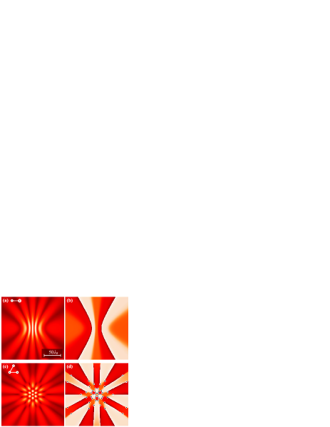
Figure 5: (Color online) (a,c) Amplitude $|\Psi|$ and (b,d) associated phase $\chi$ from Eq. (4) at $z_{0}\!\!=\!\!25\lambda_{0}$ with different source arrangements, shown pictographically alongside the (a) and (c) labels. Small circles overlaid on numerical simulations show the vortex locations as approximated by Eqs (13) and (17). Values in (a, c) are represented by linear levels from dark to light (minimum to maximum). The phase ranges from $-\pi$ (dark) to $\pi$ (light). All sources are in phase (i.e. $\phi_{2}\!\!=\!\!\phi_{3}\!\!=\!\!0$), $\lambda_{0}\!\!=\!\!\pi$ and the source arrangements are: (a,b) $r_{2}\!\!=\!\!r_{3}\!\!=\!\!3\lambda_{0},~{}\theta_{3}\!\!=\!\!0^{\circ}$. (c,d) $r_{2}\!\!=\!\!r_{3}\!\!=\!\!3\lambda_{0},~{}\theta_{3}\!\!=\!\!60^{\circ}$. Note that a spherical background has been subtracted from all phase maps, as described in the main text.

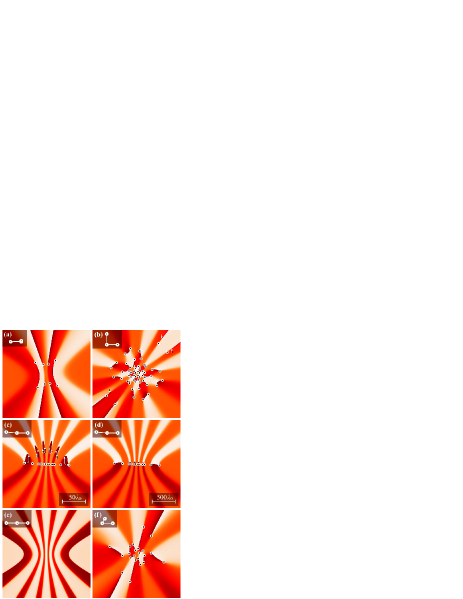
Figure 6: (Color online) Phase $\chi$ from Eq. (4) and vortex-core locations approximated by Eqs (13) and (17), with variation in source arrangement. The representation and parameters are as described in Fig. 5. The scale-bar in (c) applies to all images and corresponds to $z_{0}\!\!=\!\!25\lambda_{0}$, except for (d) which corresponds to $z_{0}\!\!=\!\!250\lambda_{0}$. Small arrows in (b,c) point to the exact vortex locations, to indicate their deviation from the far-field predictions. $\lambda_{0}\!\!=\!\!\pi$ and source arrangements are: (a) $r_{2}\!\!=\!\!r_{3}\!\!=\!\!3\lambda_{0},~{}\theta_{3}\!\!=\!\!10^{\circ}$. (b) $r_{2}\!\!=\!\!r_{3}\!\!=\!\!3\lambda_{0},~{}\theta_{3}\!\!=\!\!90^{\circ}$. (c) $r_{2}\!\!=\!\!r_{3}\!\!=\!\!3\lambda_{0},~{}\theta_{3}\!\!=\!\!175^{\circ}$. (d) $r_{2}\!\!=\!\!r_{3}\!\!=\!\!3\lambda_{0},~{}\theta_{3}\!\!=\!\!175^{\circ},~{}z_{0}\!\!=\!\!250\lambda_{0}$. (e) $r_{2}\!\!=\!\!r_{3}\!\!=\!\!3\lambda_{0},~{}\theta_{3}\!\!=\!\!180^{\circ}$. (f) $r_{2}\!\!=\!\!3\lambda_{0},r_{3}\!\!=\!\!1.5\lambda_{0},~{}\theta_{3}\!\!=\!\!60^{\circ}$. A spherical background has been subtracted from all phase maps (see main text).

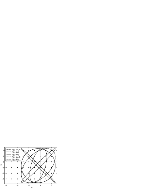
Figure 7: Parameter space ellipses corresponding to Figs 5 and 6. Enclosed lattice points define vortex locations.

The fields of view of the intensity and phase plots do not show the outermost vortex cores in most cases. This is evident from a count of the lattice points enclosed by the corresponding ellipse in Fig. 7. Only Figs 6(c) and (d) have all the generated vortices within the visible region. The corresponding parameter-space ellipse, near $-45^{\circ}$ in Fig. 7, encloses 6 lattice points — this corresponds to the $6\times 2=12$ phase vortices in Figs 6(c) and (d).

Note that, to aid visualization in all of the phase plots in Figs 5 and 6, a constant spherical background has been subtracted. Indeed, far from the three point sources, one may meaningfully write the wavefunction as a single expanding “background” spherical wave, multiplied by an envelope whose functional form depends on the particular local arrangement of the sources. By subtracting the phase of this spherical background from all of the displayed phase maps, the structure of the envelope alone — including any vortical structure — may be examined, without the distraction of a large number of concentric phase contours from the background wave. Note also that this background spherical wave corresponds to an effective source located at the geometric centroid of the real sources, with amplitude $A=A_{1}+A_{2}+A_{3}$.

Return consideration to Fig. 5(a), which exhibits a degenerate case in which two of the point sources are co-located, thereby reducing the system to two in-phase spherical sources with one having twice the amplitude of the other. As expected for only two sources, no vortices are generated. Rather, one has a series of Young-type fringes, with minima corresponding to a series of nodal planes in 3D. Each of these nodal planes is seen to constitute a “domain wall” for the phase (Pismen, 1999) [see Fig. 5(b)]. The phase is not left-right mirror symmetric, due to the positioning of the geometric centroid for three sources being to the right of center. Thus, there is a global tilt to the phase, which is observed to cycle through two branch-cuts. For this example, the parameter-space ellipse (not shown) is the limiting case of a line at $45^{\circ}$. The complementary limiting case is Fig. 6(e) where the three sources are collinear; the ellipse (not shown) is a line at $-45^{\circ}$ and again no vortices are generated. The phase here is mirror symmetric since: (i) the initial field configuration is mirror symmetric, and (ii) the wavefield propagator is rotationally symmetric. In Fig. 6(a) one of the sources has been moved just enough from coincidence with another so that the corresponding ellipse just encompasses some lattice points and vortices are created. There are four points clearly within the ellipse, giving rise to the vortices seen in the panel. If the additional two points near the boundary are just inside the ellipse, more vortices will be present at large $r_{\perp}$ and these will lie at the other ends of the branch-cut lines; otherwise the branch-cut lines will extend to infinity. Fig. 6(b) shows the case for $\theta_{3}=90^{\circ}$, giving a circle in parameter space. The number of vortices will therefore be close to the maximum for fixed values of $r_{2}$ and $r_{3}$.

The far-field solution is usually considered valid for a Fresnel number $N_{F}\equiv a^{2}/\lambda_{0}z\ll 1$, where $a$ is the largest transverse length scale present in the system (see, e.g., (Paganin, 2006)). We take this to be the maximum pinhole–pinhole spacing. The far-field condition corresponding to Fig. 5 is then $(3\lambda_{0})^{2}/\lambda_{0}z\ll 1$ or, say $z>100\lambda_{0}$. The value of $z_{0}$ for numerical simulations in Fig. 6 was deliberately chosen as $25\lambda_{0}$ to show up visual disagreements between the vortices in the numerically determined phase map and their analytically determined locations. Small arrows illustrate the true vortex positions for some vortices which do not coincide with their predicted far-field positions. The discrepancy between numerical and analytical results is highlighted in Fig. 6(c), a case arising from all parameter space lattice points lying close to the ellipse boundary. In Fig. 6(d), the Fresnel number is smaller and the correspondence is improved, but for any finite $z_{0}$, there will be some angle, close to $\pi$, at which the numerical and analytical prediction disagree by an arbitrarily large amount. Predictions are more reliable for $(m,n)$ lattice points closer to the ellipse center. In contrast with the far-field prediction that vortices may abruptly appear and disappear with infinitesimal changes in source arrangement as lattice points cross the ellipse boundary, we observe through simulations at finite $z_{0}$, that the vortex location becomes highly sensitive to source arrangement, with vortices arriving from and escaping transversely to an infinite $r_{\perp}$ distance. This point is further explored in Sec. III.8.

III.5 Source phase variation

We now consider the effects of source phase variation on the geometric parameter space description.

The functions $M(m)$ and $N(n)$ [Eqs (10)] contain the vortex coordinates’ dependency on source phase via Eqs (13) and (17), where $\phi_{j}$ is the relative phase of the $j$th source and $\phi_{1}=0$. These may be rewritten as

$$M(m)\equiv 2\pi\left[1+3\left(m-\phi_{2}/{2\pi}\right)\right]$$ (28a)

and

$$N(n)\equiv 2\pi\left[2+3\left(n-\phi_{3}/{2\pi}\right)\right],$$ (28b)

to highlight the $2\pi$ phase periodicity.

We see that a $2\pi$ change may be absorbed as an integer change in an associated parameter-space coordinate $m$ or $n$. The subtraction of a value from $m$ or $n$ corresponds geometrically to a translation of the $(m,n)$ lattice points along the associated axis, with a change of $2\pi$ effecting a translation of one lattice unit.

In summary, parameters defining the source configuration or the wave-number map to the parameter space as different ellipse constructions, whereas source phase variations correspond to translations of the lattice itself.

III.6 Estimate of number of vortices

In contrast to the case of three interfering plane waves reviewed in Sec. II, in which infinitely many nodal lines are produced, the analysis of the preceding sub-section implies that only a finite number of vortices are produced by three overlapping spherical waves, provided that there is a finite spacing between the three corresponding point sources. Here, we give a simple means to estimate the number of nodal lines, as a function of the geometry of the three point sources.

As mentioned earlier, the two-valued nature of Eq. (17) implies that each $(m,n)$ pair gives rise to a pair of vortices. Because the $m$ and $n$ values have unit spacing [see Fig. 4(b)], the number of vortices $n_{v}$ may be approximated by twice the area $\pi a^{\prime}b^{\prime}$ of the ellipse. Thus

$$n_{v}\approx 2\pi a^{\prime}b^{\prime},$$ (29)

or

$$n_{v}\approx\frac{k^{2}}{2\pi}\Big{|}r_{2}r_{3}\sin\theta_{3}\Big{|}=\frac{k^{2}\mathscr{A}}{\pi},$$ (30)

where $\mathscr{A}$ is the area of a triangle whose vertices coincide with the locations of the three point sources.

One may ask whether it is possible to develop an exact expression for the number of lattice points enclosed by our parameter-space ellipse, thereby improving on the approximation for $n_{v}$ given in Eq. (30). Indeed, this question is addressed by a famous problem in number theory known as “Gauss’s circle problem”. With $\phi_{2}=2\pi/3$, $\phi_{3}=-2\pi/3$ and $\theta_{3}=\pi/2$, the conditions corresponding to the common form of Gauss’s circle problem are established; the ellipse is a circle and is centered on a lattice point. The resulting solution for this case is both involved and well known, and so will not be given here (see, e.g., Andrews (1994)). Instead, we merely note that this establishes an unexpected and beautiful connection, between the physical system considered here, and a certain problem in the theory of numbers.

III.7 Vortex trajectories from phase variation

In most of the preceding discussion, the phases $\phi_{1},\phi_{2},\phi_{3}$ of the sources were all set to zero. Here, we consider how vortices move in response to varying the phase of one of the sources.

The equations of these curves are found by eliminating the phase $\phi_{j}$ corresponding to the source $r_{j}$ in Eqs (13) and (17). For example, the trajectories for variation of source $r_{2}$ are found by solving Eq. (13) for $\phi_{2}$ and substituting this into Eq. (17). Repeating this for $\phi_{3}$ gives a second set of trajectories along which the vortices move with $\phi_{3}$ variation. The resulting equations are

$$r_{\perp m}=\frac{M(m)\ z_{0}}{\sqrt{(3kr_{2}\cos\theta_{m})^{2}-M(m)^{2}}}$$ (31a)

and

$$r_{\perp n}=\frac{N(n)\ z_{0}}{\sqrt{(3kr_{3}\cos(\theta_{n}-\theta_{3}))^{2}-N(n)^{2}}},$$ (31b)

where the subscripts $mn$ have been changed to $m$ or $n$ to highlight the independence of the equations with respect to the complementary parameter space coordinate. Note that Eq. (31a) is the same as Eq. (15), with minor manipulation.

Fig. 8 shows the trajectories overlaying the numerical simulation results for the source arrangement seen in Fig. 6(f).

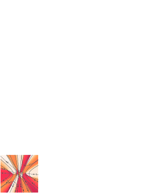
Figure 8: (Color online) Vortices move with varying source phase along trajectories and lie at the intersections of two independent sets of hyperbolas. Two independent phases give rise to two sets of hyperbolas indexed by $m$ (solid lines) and $n$ (dashed lines) respectively. The hyperbolas are shown overlaying phase $\chi$ from Eq. (6). Note that the result of this equation is $\geq 0$ for arbitrary $(r_{\perp},\theta)$. The parameters are the same as Fig. 6(f).

We have seen (Sec. III.5) that variation of $\phi_{2}$ (or $\phi_{3}$) corresponds to a translation of the $m$ (or $n$) lattice alone. Thus, our choice to eliminate the respective phase has led to the separation of the $m$ and $n$ dependence. The equations describe hyperbolas, where the polar coordinate system origin is centred between the two hyperbola branches. Note that this polar form is less common than that typically seen in the study of conics, in which the origin is placed at the focus of one branch. Eqs (31) may be thought of as a (one-to-many) mapping from lines of constant $m$ or $n$ in parameter space to hyperbolas in real space.

The angle $\theta_{3}$ in Eq. (31b) corresponds to the rotation of the $n$-indexed hyperbola axes with respect to the coordinate system axes. The square-root limits the range of real solutions, hence the number of hyperbolas and the number of vortices. The domain of the parameter-space variable $m$ (or $n$) is restricted to match that determined by the parameter-space ellipse. Thus these equations may be applied to determine the valid domains of $m$ or $n$ independently, without recourse to the ellipse solution.

Fixing the source phases defines two particular hyperbolas corresponding to the parameter space coordinates $m$ and $n$ respectively, with vortices located at the intersections of an $m$ and an $n$ curve. Both branches are included, giving four separate curves. Where one branch of an $m$ (or $n$) hyperbola intersects both branches of an $n$ (or $m$) hyperbola, only one intersection is observed to correspond to a physical vortex solution.

These equations also describe an intersecting curvilinear coordinate system. The location of a vortex on the phase map may be thought of as addressable by selection of a particular patch having coordinates $(m,n)$ and then finely addressable within that patch by variation of the source phases. Variation of the phases from 0 to $2\pi$ shifts the vortices along one of the two families of curvilinear trajectories within the patch. When there are a moderate or large number of vortices present, the patches in the central region of the phase map are correspondingly small. In this case, the vortices shift a small distance with changing phase. In the outer, sparsely populated regions, small changes in phase lead to arbitrarily large distance changes since the outermost patches have boundaries at infinity.

It is not unexpected that vortices should lie along intersecting hyperbolas. Two point sources naturally give rise to surfaces of constant phase that are hyperboloids of two sheets having the sources as their foci. The difference in path length being constant establishes the condition for constant phase and is equivalent to the well known geometric construction method for hyperboloids. The intersections of hyperboloids of two sheets with the $z=z_{0}$ plane will be hyperbolas of two branches. These will not have phase values at the amplitude maxima or minima due to any individual pair, but will be at some other value $\chi=a+ib$ on one set and $-\chi=-a-ib$ on the other, summing to zero at the vortex locations.

III.8 The parameter space near collinearity

Here we examine the behaviour of the nodal lines as $\theta_{3}$ approaches $\pi$ (three collinear sources) when $\phi_{2}=\phi_{3}=0$, since we observe a marked deviation between numerical simulation and analytical results in this regime [see Fig. 6(c), which clearly illustrates this discrepancy].

An analysis around $\theta_{3}=\pi$ may be performed by substituting $\theta_{3}=\pi+\varepsilon$ into Eq. (12), where $\varepsilon$ is small:

$$\dfrac{r_{3}}{r_{2}}\left(\vphantom{\dfrac{r_{3}}{r_{2}}}\cos(\pi+\varepsilon)+\tan\theta\sin(\pi+\varepsilon)\right)=\dfrac{N(n)}{M(m)}.$$ (32)

Applying the small-angle approximations $\cos\varepsilon\sim 1$, $\sin\varepsilon\sim\varepsilon$, Eq. (32) yields

$$\tan\theta_{mn}(\varepsilon)=\dfrac{1}{\varepsilon}\left(\dfrac{r_{2}}{r_{3}}\dfrac{N(n)}{M(m)}+1\right)$$ (33)

for the $\theta_{mn}$ coordinate of the vortex core. Substituting into Eq. (15) and applying Eq. (16) gives $r_{\perp mn}$ for our special case

$${r_{\perp mn}}^{2}=\dfrac{{z_{0}}^{2}}{\left(\dfrac{3kr_{2}}{M(m)}\right)^{2}\dfrac{1}{1+\tan^{2}\theta_{mn}}-1}.$$ (34)

Finally, substituting Eq. (33), we get

$$r_{\perp mn}(\varepsilon)=\pm\dfrac{z_{0}}{\sqrt{\dfrac{\big{(}3kr_{2}/M(m)\big{)}^{2}}{1+\dfrac{1}{\varepsilon^{2}}\left(\dfrac{r_{2}}{r_{3}}\dfrac{N(n)}{M(m)}+1\right)^{2}}-1}}.$$ (35)

In the limit $\varepsilon\rightarrow 0$, we now see that $\theta_{mn}(\varepsilon)\rightarrow\pi/2$ and $r_{\perp mn}(\varepsilon)\rightarrow\mp iz_{0}$. Regarding the latter limit, $r_{\perp mn}(\varepsilon)$ first approaches infinity and then becomes imaginary.

We may widen the context of this result by realizing that it is but one example of a lattice point crossing an ellipse boundary. Whenever this occurs, the far-field prediction is that associated vortices will be created or destroyed instantaneously. In contrast, in numerical simulations, which are at some finite distance from the source, vortices rapidly enter from or escape to infinity.

III.9 Relation to the Young’s three-pinhole interferometer

Here we show how the to map our results for three spherical point sources, hitherto the main subject of this paper, onto a three-pinhole Young’s interferometer. In this interferometer, coherent radiation illuminates a black screen that is punctured with three small pinholes, with the resulting transmitted radiation being observed at a distance that is large compared to the spacing between the pinholes. Note that the assumptions of equal amplitude and a single wavenumber, applied in Eq. (6), correspond to uniform illumination of the screen. The following argument is based on the Rayleigh–Sommerfeld diffraction theory (see, e.g., (Born and Wolf, 2003)).

The Rayleigh–Sommerfeld diffraction integral of the first kind yields a rigorous solution to the time-independent Schrödinger equation (Helmholtz equation) in a vacuum-filled half-space, for a field that obeys the Sommerfeld radiation condition. For a field $U^{(i)}$ incident on an aperture $A$ centered on the plane $z=0$, the wavefunction $U$ may be determined at an arbitrary point $(x,y,z)$ in the half-space $z\geq 0$. With the boundary conditions that $U(x,y,z=0)\approx U^{(i)}(x,y,z=0)$ when $(x,y,z=0)$ is in $A$, and $U(x,y,z=0)\approx 0$ when $(x,y,z=0)$ is not in $A$, the diffraction integral reads:

$$U(x,y,z)=\int\!\!\!\int_{A}U^{(i)}(x^{\prime},y^{\prime},0)\ K(x,y,x^{\prime},y^{\prime})\ dx^{\prime}dy^{\prime},$$ (36)

where

$$K\equiv\frac{1}{2\pi}\frac{\partial}{\partial z}\left(\frac{\exp\left(ikr\right)}{r}\right)$$ (37)

is a propagator and $r=\sqrt{(x-x^{\prime})^{2}+(y-y^{\prime})^{2}+z^{2}}$. Evaluation of the derivative gives

$$K=\frac{1}{2\pi}\frac{z}{r}\left(\frac{ik}{r}-\frac{1}{r^{2}}\right)\exp\left(ikr\right).$$ (38)

For a pinhole aperture, $U^{(i)}\equiv\delta(x-x^{\prime},y-y^{\prime},z)$, and the wavefield $U(x,y,z)$ takes the form of the propagator, Eq. (38). In general, the pinhole aperture does not produce spherical waves. However, when the observation point is such that $r\gg\lambda_{0}$, the first term in parentheses dominates the second, giving

$$K\approx\frac{ikz}{2\pi r^{2}}\exp\left(ikr\right).$$ (39)

It can now be seen that Eq. (7), which resulted from factoring out a common $\exp\left(ikr\right)/r$ term, would be unchanged by instead factoring out a common term of $ikz\exp\left(ikr\right)/2\pi r^{2}$. Similarly, when one is both in the far-field and close to the $z$-axis, $z\approx r$, so Eq. (39) reduces to a spherical wavefunction with a constant multiplier, as asserted.

In summary, the analysis of the preceding sections may be mapped onto the case of a Young’s three-pinhole interferometer, in the far field. The nodal planes of the two-pinhole Young’s experiment, which are unstable with respect to perturbations, therefore decay into a nodal-line network of vortex cores when the third pinhole is added.

IV Conclusion

A network of phase vortices was seen to be generated by the superposition of three stationary-state sources of outgoing spherical waves. We presented an analysis of the structure of the associated vortex cores (nodal lines), in the far-field regime. A finite number of vortices was seen to be generated. Determination of the number of such vortices was mapped onto the problem of determining how many points, on a two-dimensional cubic lattice, lie within a given ellipse. The equation of the ellipse depends in a known way on the geometry of the sources. The parameter space description also gives some insight into the effects of varying both the arrangement of the three sources, and their relative phase. Indeed, phase variation of two of the sources provides a means for precisely positioning one or several vortex cores. Lastly, we showed how to map all of the preceding analyses onto the problem of determining the far-field disturbance that results when a three-pinhole Young’s interferometer is coherently illuminated. In contrast to the classical two-pinhole Young’s interferometer, in which the resulting diffracted field vanishes over a series of nodal planes, the three-pinhole interferometer yields a quite different phase topology, permeated with a rich structure of nodal lines that thread vortex cores.