Transfer of d-Level quantum states through spin chains by random swapping
         A. Bayat ,         V. Karimipour

Department of Physics,

Sharif University of Technology,

P.O. Box 11365-9161,

Tehran, Iran

We generalize an already proposed protocol for quantum state transfer to spin chains of arbitrary spin. An arbitrary unknown $d-$ level state is transferred through a chain with rather good fidelity by the natural dynamics of the chain. We compare the performance of this protocol for various values of $d$. A by-product of our study is a much simpler method for picking up the state at the destination as compared with the one proposed previously. We also discuss entanglement distribution through such chains and show that the quality of entanglement transition increases with the number of levels $d$.

PACS Numbers: 03.67.Hk, 03.65.-w, 03.67.-a, 03.65.Ud.

1 Introduction

Since the proposal of S. Bose [1] for transferring quantum states via natural evolution of quantum spin one-half chains, there have been many types of extensions of this idea in various directions. For example it has been shown that perfect transfer is possible for a special class of Hamiltonians, called mirror-periodic [2, 3]. It has also been shown that one can achieve better fidelities either by using multiple chains [4] or by allowing the parties to have access to more than one site of the chain [5] or by using chains with longer range interaction than nearest neighbor [6]. The effect of thermal fluctuations [7] and decoherence [8, 9] have also been taken into account. Some other aspects of this protocol have been studied in [10, 11, 12].
However to our knowledge there has been no attempt to generalize this proposal to chains of particles of arbitrary spin. The aim of this paper is to extend this proposal in this new and fundamental direction. There are good reasons why such an extension is worthwhile. First, until a particular experimental proposal for qubit quantum computer is widely accepted as the platform for implementation of quantum computers, we have to formulate various theoretical protocols for particles with arbitrary number of levels, the so-called qudits. In fact for this reason, various protocols of quantum computation and information, like cloning [13, 14], cryptography [15] and teleportation [16, 17] have been generalized to $d$- dimensional systems. Second, from purely theoretical point of view we will learn very much in developing a particular scheme like quantum state transfer in a way such that the role of dimensionality can be studied in detail. In fact the work of Bose [1] can be rephrased in a way which demands such an extension in a quite natural way: It is well known that a quantum state can be transferred perfectly through a chain by sequential application of the swap operator defined as $P|\alpha,\beta\rangle=|\beta,\alpha\rangle$. However this method requires control on every qubit throughout the chain. Instead in [1] a state is coupled to left hand side of a spin one-half chain, governed by a ferromagnetic Heisenberg Hamiltonian

$$H=-J\sum_{i}{\bf S}_{i}\cdot{\bf S}_{i+1}+B\sum_{i=1}^{N}S_{iz},$$

where $S_{i}=\frac{1}{2}\sigma_{i}$, $\sigma_{i}$’s are the Pauli operators, $J>0$ is the coupling constant and $B$ is the magnetic field. Then the natural evolution of this chain will transfer the state to the right hand side, with a good fidelity provided that the state is extracted at an optimal time. This method can be named random swapping of a state. The reason is that using the identity

$$P=\frac{1}{2}(I+\vec{\sigma}\cdot\vec{\sigma}),$$

where $P$ is the permutation operator ($P|\alpha,\beta\rangle=|\beta,\alpha\rangle$), and a suitable redefinition of constants, $H$ can be rewritten as

$$H=-J\sum_{i}P_{i,i+1}+B\sum_{i=1}^{N}S_{iz},$$ (1)

On the sector with fixed total spin $S_{z}$, the evolution operator is equivalent to $U=e^{iJt\sum_{i}P_{i,i+1}}$, where we have set $\hbar=1$ and ignored an overall phase. Thus for an infinitesimal time step $\epsilon$, we have

$$|\psi(t+\epsilon)\rangle=|\psi(t)\rangle+\sum_{i}iJ\epsilon P_{i,i+1}|\psi(t)\rangle,$$

which shows that the state $|\psi(t+\epsilon)\rangle$ is obtained by adding to $|\psi(t)\rangle$ an equal superposition of states in which the spins of two adjacent sites have been swapped, hence the name random swapping. Thus the result of [1] can be rephrased in the following form: for qubits, random swapping achieves a fidelity which is reasonably good compared to that of sequential swapping (for which $U=\prod_{i}P_{i,i+1}$). In particular when the length of the chain is 4, the results of [1] imply that sequential and random swapping attain almost equal fidelity. Once interpreted in this way, we can ask naturally what form this comparison takes for states of arbitrary dimensions.
We should note that the Hamiltonian (1) can always be expressed in terms of nearest-neighbor scalar spin interaction terms although in each dimension it takes a specific form, for example in dimension $d=3$, it takes the form

$$H=-J\sum_{i}\left({\bf S}_{i}\cdot{\bf S}_{i+1}+({\bf S}_{i}\cdot{\bf S}_{i+1})^{2}\right)+B\sum_{i=1}^{N}S_{iz}.$$

We will find that for a fixed distance, the fidelity decreases with dimension $d$, but reaches a saturated value depending on the distance and when the sender and the receiver are 4 sites apart, nearly perfect transfer is possible for any dimension $d$. As a by-product of our study, we will propose a much simpler method for state transfer, one in which the magnetic field is kept to a vanishingly small value, instead of tuning it to a distance-dependent value as in the original protocol of [1]. The structure of this paper is as follows. In section 2 we introduce the basic protocol in $d$ dimensions, and derive the basic relations that we need in the sequel. In section 3 we study the problem of entanglement distribution in such chains. In section 4 we conclude with a discussion.

2 Quantum state transfer in chains of qudits

Originally the problem of state transferring was considered for an open chain[1]. However in that same work it was shown that in a ring of size $2N$ one can as efficiently transfer states as in an open chain as long as the distance between the sender and the receiver is not longer than $N$. To use the the advantage of simplicity of eigenfunctions of the Hamiltonian, we consider a periodic chain of length $N$, where each site comprises a state of a $d$ level system with basis states $|\mu\rangle,\ \ \mu=0,1,\cdots,d-1$. The evolution of the chain is governed by the Hamiltonian,

$$H=\frac{-J}{2}\sum_{i=1}^{N}(P_{i,i+1}-1)+B\sum_{i=1}^{N}S_{iz},$$ (2)

where the operator $P_{i,i+1}$ is the permutation operator on sites $i$ and $i+1$, and $S_{iz}$ is a diagonal operator acting on the states of site $i$ as, $S_{z}|\mu\rangle=\mu|\mu\rangle,$ for $\mu=0,1,...,d-1.$ Note that $S_{z}$, when shifted suitably, plays the role of the third component of the spin operator. Thus $B$ plays the role of a magnetic field in the $z$direction. The Hamiltonian (2) reduces to the Heisenberg Hamiltonian for spin $1/2$ states, and to the bilinear-biquadratic hamiltonian for spin $1$. For other spins it contains high power of the term $({\bf S}_{i}\cdot{\bf S}_{i+1})$. We assume that $B$ is positive.

The ground state of this Hamiltonian is given by $|{\bf 0}\rangle=|0\rangle^{\otimes N}$ with energy $E_{g}=0$.
The reason is the following. Since the permutation operator has the property $P^{2}=I$, its eigenvalues are $\pm 1$, and the operator $J(1-P_{i,i+1})$ will be a positive operator with eigenvalues $0$ and $2J$. Therefore in the absence of magnetic field, the Hamiltonian, being a sum of positive operators, is positive and since the states $|\mu\rangle^{\otimes}$, $\mu=0,\cdots d-1$ all have zero energy, they form the degenerate ground state of $H(B=0)$. The magnetic field only removes the degeneracy and lowers the energy of the state $|0\rangle^{\otimes N}$, with respect to others (note that in our notation $|0\rangle$ has the lowest value of spin component.) Since the Hamiltonian commutes with $S_{z}$, and $H(B=0)$ can be diagonlaized in sectors with fixed $z$ component of spin, this argument is valid for all values of the magnetic field $B$.

We should stress that in the absence of magnetic field, the phase diagram (i.e. the character and long range order in the ground state) of (2), may be quite complicated. This will then affects crucially the quality of state transfer in such chains, a problem which has been recently investigated for spin 1 chains in [18]. In the presence of magnetic field however, the ground state has a simple ferromagnetic order given by the ground state $|0\rangle^{\otimes N}$.

Let us denote a state in which the $i$-th site has been exited to the level $\mu$ by $|\mu_{i}\rangle$, i.e.

$$|\mu_{i}\rangle=|0,\cdots 0,\mu,0,\cdots 0\rangle.$$

The permutation operators in $H$ only displace this state through the chain and hence the Hamiltonian can be diagonalized in each sector in which the number and type of excited local states is fixed. This is a consequence of a number of conservation laws, namely

$$[H,Q^{m}]=0\ \ \ \ \ ,\ \ \ \ \ Q^{(m)}:=\sum_{i=1}^{N}(S_{z,i})^{m}$$

for $m=1,2,\cdots,d-1.$ In $d=2$ dimensions only the $Q^{(1)}$ charge is conserved. These conservation laws imply for example that a state like, $|1,1,\cdots 0,0,0\rangle$ can not evolve to a state like $|2,0,0\cdots,0,0,0\rangle$, since although their $Q^{(1)}$ charge are equal they have different $Q^{(2)}$ charges.
The states with only one site excited are called one particle states and the subspace spanned by these vectors comprise the one-particle sector of the full Hilbert space. Let us denote by $V_{1}^{(\mu)}$ the one particle sector with $Q^{(1)}$ charge equal to $\mu$. The whole one particle sector is

$$V_{1}=V_{1}^{(1)}\oplus V_{1}^{(2)}\oplus\cdots V_{1}^{(d-1)}.$$

The Hamiltonian can be diagonalized in $V_{1}^{(\mu)}$ with eigenvectors given by,

$$|E^{m}_{\mu}\rangle=\frac{1}{\sqrt{N}}\sum_{k=1}^{N}e^{\frac{i2\pi km}{N}}|\mu_{k}\rangle,\hskip 28.45274ptm=1,2,...,N,$$

with energy given by $E^{\mu}_{m}=J-Jcos(\frac{2\pi m}{N})+B\mu.$ For quantum state transferring we can consider site $s$ as the sender of the system and site $r$ as a receiver. The initial state that should be sent is

$$|\psi_{s}\rangle=\sum_{\mu=0}^{d-1}a_{\mu}|\mu\rangle.$$

So the initial state of the system (the site $s$ plus the chain) is,

$$|\psi(0)\rangle=|\psi_{s}\rangle\otimes|\textbf{0}\rangle=a_{0}|\textbf{0}\rangle+\sum_{\mu=1}^{d-1}a_{\mu}|\mu_{s}\rangle.$$

In view of the fact that $H|\textbf{0}\rangle=0$, the state at time $t$ will be,

$$|\psi(t)\rangle=a_{0}|\textbf{0}\rangle+\sum_{\mu=1}^{d-1}a_{\mu}e^{-iHt}|\mu_{s}\rangle=a_{0}|\textbf{0}\rangle+\sum_{k=1}^{N}\sum_{\mu=1}^{d-1}f_{ks}a_{\mu}e^{-iB\mu t}|\mu_{k}\rangle.$$

In deriving this formula we have used the fact that $[S_{z},\tilde{H}:=\sum_{i}P_{i,i+1}]=0$ and the conservation laws which restricts the evolution to the one particle sector of fixed $Q^{(1)}$ charges. We have also defined

$$f_{ks}:=\langle\mu_{k}|e^{-i\tilde{H}t}|\mu_{s}\rangle,$$

which is indeed independent of $\mu$ and hence can be taken outside the sum.

The state of site $r$ which is acting as the receiver will be generally mixed, so is denoted by $\rho_{r}(t)$ and is obtained by tracing out the other sites.

$$\rho_{r}(t) = tr_{\hat{r}}{|\psi(t)\rangle\langle\psi(t)|}=(1-\sum_{\mu=1}^{d-1}|a_{\mu}|^{2}|f_{rs}^{\mu}|^{2})|0\rangle\langle 0|+\sum_{\mu=1}^{d-1}a_{0}a_{\mu}^{*}f_{rs}^{\mu*}|0\rangle\langle\mu|$$

$$+ \sum_{\mu=1}^{d-1}a_{0}^{*}a_{\mu}f_{rs}^{\mu}|\mu\rangle\langle 0|+\sum_{\mu,\nu=1}^{d-1}a_{\mu}a_{\nu}^{*}f_{rs}^{\mu}f_{rs}^{\nu*}|\mu\rangle\langle\nu|.$$

Rearrangement of the right hand side yields

$$\rho_{r}(t)=(1-P)|0\rangle\langle 0|+P|\phi\rangle\langle\phi|,$$

where

$$P=|f_{rs}|^{2}(1-|a_{0}|^{2})+|a_{0}|^{2},$$

and

$$|\phi\rangle=\frac{1}{\sqrt{P}}(a_{0}|0\rangle+f_{rs}\sum_{\mu=1}^{d-1}a_{\mu}e^{-iB\mu t}|\mu\rangle).$$

Alternatively we can say that the input state $\rho_{s}(0)$ is mapped to the output state $\rho_{r}(t)$ by the positive map

$$\rho_{r}(t)=\sum_{\mu}A_{\mu}\rho_{s}(0)A_{\mu}^{\dagger},$$

where the so-called Kraus operators $A_{\mu}$ are given by

$$A_{0}=|0\rangle\langle 0|+\sum_{\mu=1}^{d-1}f_{rs}^{\mu}\ \ |\mu\rangle\langle\mu|,\ \ \ \ A_{\mu}=\sqrt{1-|f_{rs}^{\mu}|^{2}}\ \ \ |0\rangle\langle\mu|,\ \ \ \ \ \mu=1,...,d-1.$$ (4)

The fidelity between the received state $\rho_{r}(t)$ and the initial state $\rho_{s}(0)=|\psi_{s}\rangle\langle\psi_{s}|$ is defined by $F=|\langle\psi_{s}|\rho_{r}(t)|\psi_{s}\rangle|^{2}$ which turns out to be

$$F(t)=|a_{0}|^{2}+\sum_{\mu=1}^{d-1}|a_{0}|^{2}|a_{\mu}|^{2}\{1-|1-f_{rs}^{\mu}|^{2}\}+\sum_{\mu,\nu=1}^{d-1}|a_{\mu}|^{2}|a_{\nu}|^{2}f_{rs}^{\mu}f_{rs}^{\nu*}.$$

In the sequel we should maximize this fidelity when it is uniformly averaged over the input states. The average is defined by

$$\langle F(t)\rangle=\int F(t)dU,$$

where $dU$ is an invariant (Haar) measure over the $SU(d)$ group, normalized such that $\int dU=1$. The reason for this choice of measure is as follows. Let us fix a basis, like $\{|0\rangle,|1\rangle,\cdots|d-1\rangle\}$. We take a fixed reference state like $|0\rangle$ and note that every arbitrary state $|\psi\rangle$ can be obtained from $|0\rangle$ by the action of a unitary operator $U$, i.e. $|\psi\rangle=U|0\rangle$, for some non-unique $U\in SU(d)$. However, any two unitary matrices $U$ and $Ug$, where $g\in SU(d-1)$ leaves $|0\rangle$ invariant, lead to the same state $|\psi\rangle$. Therefore a proper measure that prevents this multiple counting is a measure over $U(d)/U(d-1)$. However since every state is multiply counted equally ( by a factor which is exactly the volume of the group $SU(d-1)$), this does not affect the final averaging and we can use the simple measure over $U(d)$. Invariance of this measure under left multiplication, i.e. $dU=d(gU)$ guarantees uniformity of the measure over the space of all states. In two dimensions one can avoid multiple counting in a simple way, since in this case $U(2)/U(1)\sim SO(3)/SO(2)\sim S_{2}$ and therefore, one can use the measure over the 2 dimensional (Bloch) sphere to count every state once. This is the measure used by Bose in [1].
For a $d-$ dimensional normalized state $|\psi\rangle=\sum_{\mu=0}^{d-1}a_{\mu}|\mu\rangle$ an invariant measure yields trivially $\langle|a_{\mu}|^{2}\rangle=\frac{1}{d}\ \ \forall\mu$. To calculate the other averages we use $|\psi\rangle=U|0\rangle$ and write

$$\langle|a_{\mu}|^{4}\rangle=\langle|a_{0}|^{4}\rangle=\int|U_{00}|^{4}dU=\frac{2}{d(d+1)},\ \ \ \forall\ \ \mu,$$

where for the last equality we have used a result from [19] on invariant integration on unitary groups. We can now calculate $\langle|a_{\mu}|^{2}|a_{\nu}|^{2}\rangle$ for $\mu\neq\nu$. In view of the normalization of the state, we have

$$1 = \sum_{\mu,\nu}\langle|a_{\mu}|^{2}|a_{\nu}|^{2}\rangle=\sum_{\mu}\langle|a_{\mu}|^{4}\rangle+\sum_{\mu\neq\nu}\langle|a_{\mu}|^{2}|a_{\nu}|^{2}\rangle$$

$$= d\frac{2}{d(d+1)}+d(d-1)\langle|a_{\mu}|^{2}|a_{\nu}|^{2}\rangle,$$

thus we find

$$\langle|a_{\mu}|^{2}|a_{\nu}|^{2}\rangle_{\mu\neq\nu}=\frac{1}{d(d+1)}.$$

Using these results we can now calculate the average of fidelity over a uniform ensemble of input states.

$$\langle F(t)\rangle=\frac{1}{d}+\frac{1}{d(d+1)}\sum_{\mu=1}^{d-1}({f_{rs}^{\mu}+{f^{*}}_{rs}^{\mu}})+\frac{1}{d(d+1)}\sum_{\mu,\nu=1}^{d-1}f_{rs}^{\mu}{f^{*}}_{rs}^{\nu}.$$ (6)

In order to write $\langle F(t)\rangle$ in a simple form we note that

$$|\sum_{\mu=1}^{d-1}f^{\mu}_{rs}|=|\sum_{\mu=1}^{d-1}e^{-i\mu Bt}f_{rs}|=|f_{rs}|\Gamma_{d}(Bt),$$

where

$$\Gamma_{d}(Bt):=\frac{\sin\frac{(d-1)Bt}{2}}{\sin\frac{Bt}{2}},$$

and

$$\sum_{\mu=1}^{d-1}(f^{\mu}_{rs}+{f^{*}}^{\mu}_{rs})=2\cos(\gamma_{rs}-\frac{dBt}{2})\Gamma_{d}(Bt),$$

where $f_{rs}=|f_{rs}|e^{i\gamma_{rs}}$. Inserting these in (6) we find that

$$\langle F(t)\rangle=\frac{1}{d}+\frac{2}{d(d+1)}|f_{rs}|\cos(\gamma_{rs}-\frac{dBt}{2})\Gamma_{d}(Bt)+\frac{1}{d(d+1)}|f_{rs}|^{2}\Gamma_{d}^{2}(Bt).$$ (7)

For $d=2$ we recover the formula of [1].

It remains to calculate the explicit expression for the amplitudes $f_{rs}^{\mu}$. We note that

$$f_{rs}=\langle\mu_{r}|e^{-i\tilde{H}t}|\mu_{s}\rangle=\sum_{k=1}^{N}\langle\mu_{r}|e^{-i\tilde{H}t}|E^{\mu}_{k}\rangle\langle E^{\mu}_{k}|\mu_{s}\rangle=\frac{e^{-iJt}}{N}\sum_{k=0}^{N-1}e^{iJtcos(\frac{2\pi k}{N})}e^{\frac{i2\pi k(r-s)}{N}}.$$

For large $N$, a closed formula for $f_{rs}$ can be obtained by writing the right hand side as an integral. Thus

$$f_{rs}\approx\frac{e^{-iJt}}{2\pi}\int_{0}^{2\pi}e^{iJtcos(\theta)+i\theta(r-s)}=e^{-i(Jt-\frac{\pi}{2}(r-s))}J_{r-s}(Jt),\ \ \ {\rm{Large}}\ \ N,$$

where $J_{n}$ is the Bessel function of the first kind of order $n$. It now remains to follow a definite strategy for picking up the state at the destination point $r$. As is clear from equation (7), there is a distinctive difference between dimension $d=2$ and any other dimension, since in $d=2$ we have $\Gamma_{2}(Bt)=1$ and the magnetic field enters only in one single term, namely the argument of cosine function. (Note that we can always re-scale the other coupling constant $J$ to 1.) Thus in $d=2$ there is rather a unique strategy, first suggested in [1]: at any given time $t$ one finds the magnitude of $B=B(t)$ which maximizes the cosine function to unity and then searches among the values of time $t$ to determine the optimal time $t_{opt}$ for picking up the state. This will then determine the optimal value of the magnetic field through the relation $B_{opt}=B(t_{opt}).$ Note that since $t_{opt}$ depends on the distance $r-s$ between the sender and the receiver, the optimal value of the magnetic field also depends on this distance. This is an inconvenient feature of this strategy.

A by-product of the present work is that a much simpler strategy can be used, namely: tune the magnetic field to a vanishingly small value, then the optimal time for picking up the state is almost independent of the magnetic field. To see this we note that for higher values of $d$, the magnetic field enters in two different ways in the final formula for the average fidelity, namely in the argument of the cosine function as in $d=2$ and in the function $\Gamma_{d}(Bt)$. These two functions may have incompatible properties so that they may not be maximized simultaneously. The latter function is maximized when its argument $Bt$ goes to zero, while the former function has a complicated dependence on $t$ and $B$ separately. Thus one can follow two different strategies for picking up the states at point $r$, the first one is exactly the same as in [1], explained above. We can also follow a second much simpler strategy, which has the advantage of no need for distance-dependent tuning of the magnetic field. We simply apply a vanishingly small magnetic field ($Bt<<1$) for all the times involved in the transfer process. On the other hand $B$ should not be vanishing so that we have a unique ferromagnetic ground state. This maximizes the function $\Gamma_{d}(Bt)$ to $\approx(d-1)$. We are now left with a function which is entirely a function of $t$ and can find for any distance $r-s$, the optimal time and the maximum average fidelity.
In figure (1), we show the average fidelity for transferring $d=2,3,$ and $4-$ level states through half way distances in closed rings, using this strategy and compare it with the original Bose strategy. Thus when $r-s=20$, we are using a ring of size $N=40$.

There are a few interesting features. First it is seen that the average fidelity is almost the same in both strategies, which implies that we can always, even for $d=2$, use the second method which is much simpler and does not rely on distance-dependent tuning of magnetic fields. Second we note that the strong similarity of the fidelity curves in various dimensions. To see the reason of this universality, we note that for very small magnetic fields, $Bt<<1$, where $\Gamma_{d}(Bt)\sim(d-1)$, the average fidelity behaves as

$$\langle F(t)\rangle\sim\frac{1}{d}+\frac{2(d-1)}{d(d+1)}|f_{rs}|\cos(\gamma_{rs})+\frac{(d-1)^{2}}{d(d+1)}|f_{rs}|^{2}.$$ (8)

The curves in figure (1) show the fidelities at the optimal time $t_{op}$ where $\langle F(t_{opt})\rangle$ becomes a maximum, obtained by numerical searches in a time span $t\in(0,400)$. Let us now suppose that the optimal time is the time where $\cos(\gamma_{rs})\approx 1$. Since $f_{rs}$ is independent of $d$, we can obtain a universal relation for optimal fidelities from the above equation by rewriting it as follows. First we note from the above equation that

$$F^{*}_{opt}:=\lim_{d\longrightarrow\infty}\langle F_{opt}\rangle=|f_{rs}|^{2}.$$

Rearranging the terms of (8) after setting $\cos\gamma_{rs}\approx 1$, we find

$$\frac{\sqrt{d(d+1)\langle F_{opt}\rangle-d}-1}{d-1}=\sqrt{F^{*}_{opt}},$$ (9)

which is a constant. To check this assumption and the resulting universality, we draw in figure (2) the left hand side of (9) (as obtained from numerical searches for the optimal time, leading to figure (1) and not by setting $\cos\gamma_{rs}\approx 1$) for several values of $d$. The universal behavior is now completely evident.
Finally, we note that almost perfect state transfer of any $d-$ level state is possible when $|r-s|=1,2,4$. This possibility of almost perfect state transfer was first noticed in [1] for $d=2$ level states. We now see that this is a general and curious feature of random swapping for any $d-$ level state. We know that by sequential swapping at any two consecutive sites, one can perfectly transfer an unknown state through a chain. However this requires a multitude of control operations at all sites of the chain. The above result about perfect transfer over distances of $4$ sites by random swapping (induced by the natural Hamiltonian dynamics), means that one can transfer states perfectly over long distances in a chain by a smaller number of control operations, namely by 1/4 of the number of sites of the chain.

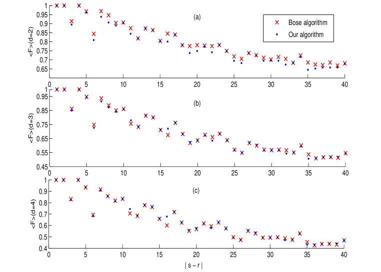
Figure 1: (Color online) The average fidelity for transferring d=$2,3$ and $4-$ level states for two different strategies explained in the text. In each case the distance between the sender (s) and the receiver (r) is half the length of the chain (N).

Figure (3) shows average fidelities for three different distances, namely $|r-s|=4,7,14$, as functions of the number of levels $d$. It is seen that the average fidelity decreases with $d$ and saturates to a constant value, depending on the distance. Plots $a$ and $b$ refer to two different strategies discussed above.

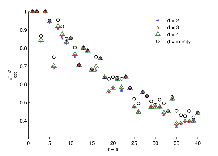
Figure 2: (Color online) The universal relation for optimal fidelities, explained in equation (9).

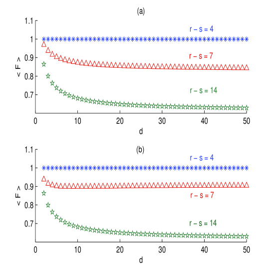
Figure 3: (Color online) The average fidelity for three different distances, namely $|r-s|=4,7,14$, as functions of the number of levels $d$. Plots $a$ are for the strategy of Bose [1] and plots $b$ are for our strategy.

3 Entanglement distribution

One of the major problems of quantum information science and technology is the distribution of entangled pairs over long distances. For flying qubits, such pairs in the form of polarization-entangled photons have been distributed to various long distances through optical fibres and free air [20, 21, 22, 23, 24, 25]. For small distances in a quantum computer, for which we supposedly will be dealing with solid state devices or ion traps in the future, one needs to distribute entangled pairs through such chains of qubits. In [1] a method was proposed for such a task, when the particles have spin $1/2$ or have two levels (qubits). Here we generalize this idea to $d-$ level states or qudits. We will see here that the quality of entanglement transfer is better for higher values of $d$.

Suppose that a maximally entangled state is prepared between sites $0$ (not coupled to the chain) and site $s$ of the chain. We want to use the natural dynamics of the chain to transfer this entanglement through the chain. In particular we want to see what will be the entanglement between sites $0$ and $r$ at time $t$. The initial states is

$$|\psi_{ME}\rangle_{0,s}=\frac{1}{\sqrt{d}}\sum_{\mu=0}^{d-1}|\mu\mu\rangle.$$ (10)

At time $t$, the joint state of sites $0$ and $r$ can be determined by the extension of the map (4) to one acting on the chain and the external site $0$:

$$\rho_{0,r}(t)\rangle=\sum_{\mu=0}^{d-1}(I\otimes A_{\mu})|\psi_{ME}\rangle\langle\psi_{ME}|(I\otimes A_{\mu}^{\dagger}).$$ (11)

Insertion of the Kraus operators $A_{\mu}$s from (4) in (11) gives,

$$\rho_{0r}(t) = \frac{1}{d}\{\ \ |00\rangle\langle 00|+\sum_{\mu=1}^{d-1}f_{rs}^{\mu*}|00\rangle\langle\mu\mu|+\sum_{\mu=1}^{d-1}f_{rs}^{\mu}|\mu\mu\rangle\langle 00|$$

$$+ \sum_{\mu,\nu=1}^{d-1}f_{rs}^{\mu}f_{rs}^{\nu*}|\mu\mu\rangle\langle\nu\nu|+\sum_{\mu=1}^{d-1}(1-|f_{rs}^{\mu}|^{2})|\mu 0\rangle\langle\mu 0|\ \ \}.$$

We use Logarithmic Negativity (LN) [26] as a measure of entanglement of the state $\rho_{0r}$ which is defined as,

$$LN(\rho_{12})=log_{2}(\|\rho_{12}^{T_{2}}\|),\ \ \ \ \|O\| = tr\sqrt{O^{\dagger}O},$$ (13)

where by the superscript ${T_{2}}$, the partial trace over the second space is implied. Logarithmic negativity is an entanglement monotone which is additive and does not increase on the average under all partial transpose preserving operations [27]. For a pure maximally entangled state like (10), equation (13) yields $LN(|\psi_{ME}\rangle)=log_{2}d$.
In order to calculate logarithmic negativity we need eigenvalues of $\rho_{0r}^{T_{r}{\dagger}}\rho_{0r}^{T_{r}}$. Straightforward calculations shows that

$$\rho_{0r}^{T_{r}{\dagger}}\rho_{0r}^{T_{r}} = \frac{1}{d^{2}}\{|00\rangle\langle 00|+\sum_{\mu=1}^{d-1}|f_{rs}^{\mu}|^{2}|\mu 0\rangle\langle\mu 0|+\sum_{\mu=1}^{d-1}|f_{rs}^{\mu}|^{2}|0\mu\rangle\langle 0\mu|$$ (14)

$$+ \sum_{\mu,\nu=1}^{d-1}|f_{rs}^{\mu}|^{2}|f_{rs}^{\nu}|^{2}|\mu\nu\rangle\langle\mu\nu|+\sum_{\mu=1}^{d-1}(1-|f_{rs}^{\mu}|^{2})^{2}|\mu 0\rangle\langle\mu 0|$$

$$+ \sum_{\mu=1}^{d-1}(1-|f_{rs}^{\mu}|^{2})f_{rs}^{\mu}|\mu 0\rangle\langle 0\mu|+\sum_{\mu=1}^{d-1}(1-|f_{rs}^{\mu}|^{2})f_{rs}^{\mu*}|0\mu\rangle\langle\mu 0|\}.$$

It is readily seen that this operator is the direct sum of two-dimensional matrices of the form

$$\frac{1}{d^{2}}\left(\begin{array}[]{cc}|f_{rs}^{\mu}|^{2}&(1-|f_{rs}^{\mu}|^{2})f_{rs}^{\mu*}\\ (1-|f_{rs}^{\mu}|^{2})f_{rs}^{\mu}&1-|f_{rs}^{\mu}|^{2}+|f_{rs}^{\mu}|^{4}\\ \end{array}\right)$$

in the subspaces spanned by $|\mu 0\rangle$ and $|0\mu\rangle$ (with eigenvalues $\frac{1}{d^{2}},\frac{|f_{rs}^{\mu}|^{2}}{d^{2}}$ ) and a diagonal matrix spanned by the rest of basis vectors. Putting these together we find the spectrum of the matrix $\sqrt{\rho_{0r}^{T_{r}{\dagger}}\rho_{0r}^{T_{r}}}$ as follows,

$$\left\{\begin{array}[]{ll}\frac{1}{d},&\ \ \ d\\ \frac{|f_{rs}^{\mu}||f_{rs}^{\nu}|}{d},&\ \ \ (d-1)^{2}\\ \frac{|f_{rs}^{\mu}|^{2}}{d},&\ \ \ d-1,\\ \end{array}\right.$$

where the number in front of each eigenvalue denotes its degeneracy. Therefore the logarithmic negativity of the final state between sites $0$ and $r$ can be computed easily. It is found that

$$LN(\rho_{0r}(t))=log_{2}\{1+\frac{1}{d}\sum_{\mu,\nu=1}^{d-1}|f_{rs}^{\mu}||f_{rs}^{\nu}|+\frac{1}{d}\sum_{\mu=1}^{d-1}|f_{rs}^{\mu}|^{2}\}$$

and because $|f_{rs}^{\mu}|$ is independent of $\mu$ so we can simplify the above formula,$LN(\rho_{0r}(t))=\log_{2}\{1+|f_{rs}|^{2}(d-1)\}$. This equation shows that with increasing $d$ the logarithmic negativity and hence the entanglement increases and indeed approaches its maximum value for continuous variable states. We can define the efficiency of entanglement distribution as a measure of the the percentage of entanglement that is gained after distribution of the maximally entangled state through the chain, so we introduce the efficiency as,

$$E=\frac{LN_{2}}{LN_{1}}=\frac{\log_{2}\{1+|f_{rs}|^{2}(d-1)\}}{log_{2}d}=\log_{d}\{1+|f_{rs}|^{2}(d-1)\}.$$

Figure (4) shows the efficiency of entanglement of sites $1$ and $30$ in a ring of size $N=60$ as a function of time for three different values of $d$.

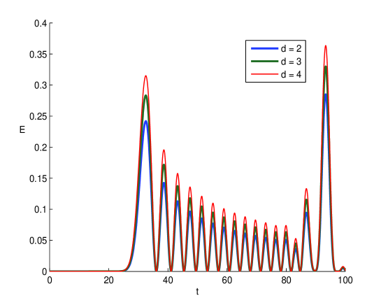
Figure 4: (Color online) Entanglement transition through a chain. The efficiency of transmission of maximally entangled pairs through a distance of 30 sites in a chain of length 60 for different $d-$ level states. The curves from bottom to top correspond to $d=2$, $d=3$ and $d=4$.

It is seen that the optimal time for picking up the states is independent of $d$ and the efficiency is increased by increasing the dimension $d$.

4 Summary

We have generalized the protocol of [1] for quantum stater state transfer of qubits to transfer of $d$-level states. On the theoretical side, we can consider the results of [1] and the present paper as an answer to the question ”with what fidelity can a quantum state be transferred through a chain if we use random swapping instead of sequential swapping?”. The latter method is known to achieve unit fidelity but requires local control at every site of the chain. We have shown that 1- the fidelity decreases with the dimension $d$, but reaches a saturated value depending on the distance, and 2- that when the sender and the receiver are 4 sites apart, nearly perfect transfer is possible for any dimension $d$. A by-product of our study is that we have proposed a much simpler method for state transfer, one in which the magnetic field is kept to a vanishingly small value, instead of tuning it to a distance-dependent value as in the original protocol of [1].
Furthermore the concept of entanglement distribution has been studied for $d$-level states and the interesting result is that the quality of entanglement distribution will be improved by increasing the dimension $d$.

5 Acknowledgement

We would like to thank the members of the quantum information group in the physics department of Sharif university for very valuable discussions.

References

- [1] S. Bose, Phys. Rev. Lett. 91, 207901 (2003).
- [2] M. Christandl, N. Datta, A. Ekert, A.J. Landahl, Phys. Rev. Lett. 92, 187902 (2004).
- [3] C. Albanese, M.Christandl, N. Datta, A. Ekert, Phys. Rev. Lett. 93,230502 (2004).
- [4] D. Burgarth, S. Bose, Phys. Rev. A 71, 052315 (2005).
- [5] V. Giovannetti, D. Burgarth, Phys. Rev. Lett. 96, 030501 (2006).
- [6] M. Avellino, A.J. Fisher, S. Bose, Phys. Rev. A 74, 012321 (2006).
- [7] A. Bayat, V. Karimipour, Phys.Rev. A 71, 042330 (2005).
- [8] D. Burgarth, S. Bose, Physical Review A 73, 062321 (2006).
- [9] J.M. Cai, Z.W. Zhou, G.C. Guo, Phys. Rev. A. 74, 022328 (2006).
- [10] T.J. Osborne, N. Linden Phys. Rev. A 69, 052315 (2004).
- [11] V. Subrahmanyam Phys. Rev. A 69, 034304 (2004).
- [12] G.De Chiara et.al., Phys. Rev. A 71, 042330 (2005).
- [13] R. F. Werner, Phys. Rev. A58, 1827(1998).
- [14] M. Keyl and R. F. Werner, J. Math. Phys. 40, 3283 (1999).
- [15] A. Acin, N. Gisin, V. Scarani, Quant. Inf. Comp. Vol.3 No. 6, 563 (2003).
- [16] G. Rigolin, Phys. Rev. A, 71(2005)032303.
- [17] X. H. Ge and Y. G. Shen, Phys. Lett. B606 (2005)184.
- [18] O. Romero-Isart, Kai Eckert, and A. Sanpera, quant-ph/0610210.
- [19] S. Aubert, C.S. Lam, J.Math.Phys. 45 (2004) 3019-3039.
- [20] N. Gisin, G. Ribordy, W. Tittel and H. Zbinden, Rev. Mod. Phys. 74, 145 (2002);
- [21] R. Ursin et.al., quant-ph/0607182.
- [22] T. Jennewein, C. Simon, G.W eihs, H. Weinfurter, A. Zeilinger, Phys. Rev. Lett. 84, 4729 (2000),quant-ph/9912117.
- [23] M. Aspelmeyer, T. Jennewein, M. Pfennigbauer, W. Leeb, A. Zeilinger, IEEE Journal of Selected Topics in Quantum Electronics 1541- 1551, quant-ph/0305105.
- [24] K.J.Resch , et.al , Opt. Express 13, 202-209 (2005), quant-ph/ 0501008 .
- [25] A. Poppe, et.al ,Opt. Express 12, 3865-3871 (2004) ,quant-ph/0404115.
- [26] G. Vidal, R.F. Werner, Phys. Rev. A 65, 032314 (2002).
- [27] M. B. Plenio, Phys. Rev. Lett. 95, 090503 (2005).