On quantum microcanonical equilibrium

Abstract

A quantum microcanonical postulate is proposed as a basis for the equilibrium properties of small quantum systems. Expressions for the corresponding density of states are derived, and are used to establish the existence of phase transitions for finite quantum systems. A grand microcanonical ensemble is introduced, which can be used to obtain new rigorous results in quantum statistical mechanics.

1 Introduction

The purpose of this paper is to examine properties of quantum systems in thermal equilibrium. Questions that arise in this context, for example, are: “What is the state of a system in equilibrium?” or “What is the temperature of an isolated system in equilibrium?” In the case of a classical system immersed in a heat bath, the equilibrium distribution takes the Gibbs form $\exp(-\beta H)/Z(\beta)$, where $\beta=1/k_{B}T$ is the inverse temperature of the bath. What about a quantum system? Is the equilibrium state given by the Gibbs density matrix $\exp(-\beta{\hat{H}})/Z(\beta)$? If so, how does one verify that the parameter $\beta$ appearing in the density matrix is the inverse temperature of the bath?

To investigate questions of this kind it is useful to consider first the classical situation. In the classical case, we take the system and the bath as a whole and regard this as a single isolated system. The Hamiltonian (symplectic) structure of classical phase space $\Gamma$ then allows us to define the density of states $\Omega(E)=\int_{\Gamma}\delta(H(x)-E){\rm d}V$ as the weighted volume of the phase space occupied by states with energy $E$. In equilibrium the state of the system maximises entropy and thus is given by a uniform distribution over the energy surface; this can be derived if the Hamiltonian evolution exhibits ergodicity. The entropy of the equilibrium state is thus given by $S(E)=k_{B}\ln\Omega(E)$, and the temperature is defined by the thermodynamic relation $T{\rm d}S={\rm d}E$. These are the necessary ingredients for the consideration of the equilibrium properties of a small subsystem. In particular, under a set of reasonable assumptions, it is possible to deduce, by use of the law of large numbers, that the equilibrium properties of a small subsystem are described by the Gibbs state. A complete derivation of these results is outlined in the seminal work of Khinchin [1]. Although the derivation of the equilibrium state is surprisingly complicated, once the relevant assumptions are specified, there are no ambiguities in the matter, and familiar results associated with the canonical ensemble can be obtained rigorously.

The situation is markedly different in the case of a quantum system. First, in the usual Hilbert space formulation of quantum mechanics it is not clear how one can exploit the Hamiltonian structure. This leads to a difficulty in defining the temperature of a closed system. Second, since no rigorous derivation of the temperature exists (at least for finite quantum systems), it is not possible to verify whether the parameter $\beta$ appearing in the Gibbs density matrix agrees with the inverse temperature of the bath.

In the literature on quantum statistics it is often postulated that the microcanonical density matrix of a quantum system with eigenenergy $E_{i}$ is given by the projection operator onto the Hilbert subspace spanned by states with that energy, normalised by the dimensionality $n_{E_{i}}$ of that subspace. The entropy is then defined by the expression $S=k_{B}\ln n_{E_{i}}$. A rigorous derivation of this density matrix is given by Khinchin [2]; however, the assumptions required to obtain the result go beyond those required for the classical case. In particular, it is necessary to forbid all superpositions of states with different energy. The exclusion of general superpositions, however, contradicts the superposition principle of quantum mechanics. This incompatibility between quantum mechanics and quantum statistical mechanics is an issue that has troubled many authors. For example, Schrödinger remarked in this connection that “. . . this assumption is irreconcilable with the very foundations of quantum mechanics”, and that “. . . to adopt this view is to think along severely ‘classical’ lines” [3]. Confronted with this apparent contradiction, Schrödinger was nonetheless able to offer an argument to show, in effect, that in thermodynamic limit (where the number of particles in the system approaches infinity) the assumption that general superpositions are forbidden is justified [3].

There is another important shortcoming in the familiar derivation of quantum statistical mechanics, namely, that the entropy is a discontinuous function of the energy. As a consequence, the temperature of a finite isolated system is undefined. This issue is addressed by Griffiths [4], who demonstrated the existence of a thermodynamic limit in which thermodynamic functions are well defined. We thus see that to make sense of the conventional approach to quantum statistics, a “macroscopic” limit is required. In this limit, however, we expect quantum systems to behave semiclassically so that superpositions, in particular, are excluded. For finite quantum systems, these issues remain unresolved.

While the notion of a thermodynamic limit was justified both theoretically and experimentally some forty years ago, there have been experiments carried out on quantum systems over the past decade that involve small numbers of particles (see Gross [5] and references cited therein). In particular, phase transitions have been observed in small systems—for example, the spherically symmetric cluster of $139$ sodium atoms exhibits a solid-to-liquid phase transition at about $267$ K [6]. Such experiments demonstrate the breakdown of the conventional approach in which phase transitions are predicted only in thermodynamic limits.

To obtain an equilibrium distribution that is well defined for finite systems, and to address the issue of the observed finite-size phase transitions, we have recently introduced an alternative formulation to quantum microcanonical equilibrium [7]. The idea is to follow the derivation of the traditional result, as outlined in Khinchin [2], as closely as possible, but to relax just one of the assumptions; namely, for a fixed energy $E$, we allow the system to be in a superposition of energy eigenstates with distinct eigenvalues.

2 Thermodynamic equilibrium

The idea of the new microcanonical equilibrium can be described heuristically as follows. We consider a gas consisting of a large number $N$ of weakly-interacting identical quantum molecules. As in the conventional approach, the intermolecular interactions are assumed strong enough to allow the gas to thermalise but weak enough so that, to a good approximation, the total system energy can be written as $\sum_{i=1}^{N}{\hat{H}}_{i}\approx{\hat{H}}_{\rm total}$, where $\{{\hat{H}}_{i}\}_{i=1,2,\ldots,N}$ are the Hamiltonians of the individual constituents. If the composite system is in isolation, then the total energy is a fixed constant: $\sum_{i=1}^{N}\langle{\hat{H}}_{i}\rangle=E_{\rm total}$. Now consider the result of a hypothetical measurement of the energy of one of the constituents. In equilibrium, the state of each constituent should be such that the average outcome of an energy measurement should be the same; that is, $\langle{\hat{H}}_{i}\rangle=E$, where $E=N^{-1}E_{\rm total}$. In other words, the equilibrium state of each constituent must lie on the energy surface ${\mathcal{E}}_{E}=\{|\psi\rangle\large|~{}\langle\psi|{\hat{H}}_{i}|\psi\rangle=E\}$ in the pure-state manifold for that constituent. Since $N$ is large, this will ensure that the uncertainty in the total energy of the composite system, as a fraction of the expectation of the total energy, is vanishingly small.

It is convenient to describe the distribution of the various constituent pure states, on their respective energy surfaces, as if we were considering a probability measure on the energy surface ${\mathcal{E}}_{E}$ of a single constituent. In reality, we have a large number of approximately independent constituents; but owing to the fact that the respective state spaces are isomorphic we can represent the behaviour of the aggregate system with the specification of a probability distribution on the energy surface of a single “representative” constituent.

In thermal equilibrium the resulting distribution should be uniform over the energy surface ${\mathcal{E}}_{E}$ since it must maximise the entropy. Therefore, the density of states is given by

$$\Omega(E)=\int_{\Gamma}\delta(H(\psi)-E){\rm d}V_{\Gamma}.$$ (1)

Here, $\Gamma$ denotes the pure state manifold and ${\rm d}V_{\Gamma}$ is the associated Fubini-Study volume element of $\Gamma$. Once $\Omega(E)$ is specified, the entropy is given by $S(E)=k_{B}\ln\Omega(E)$. It follows that the temperature and the specific heat can be deduced from thermodynamic relations $T{\rm d}S={\rm d}E$ and $C(T)={\rm d}E/{\rm d}T$. A short calculation shows that

$$k_{B}T=\frac{\Omega(E)}{\Omega^{\prime}(E)},\quad{\rm and}\quad C(T)=\frac{k_{B}(\Omega^{\prime})^{2}}{(\Omega^{\prime})^{2}-\Omega\Omega^{\prime\prime}}.$$ (2)

The advantage of the present formulation over the traditional approach is that the entropy is a continuous function of the energy. As a consequence, thermodynamic functions such as those in (2) are well defined for finite quantum systems. However, to justify the term “temperature” for the ratio $\Omega/\Omega^{\prime}$ we must show its properties are consistent with the requirements of thermodynamic equilibrium. For this purpose, consider two independent systems, each in equilibrium, with state densities $[\Omega_{1}(E_{1})]^{N_{1}}$ and $[\Omega_{2}(E_{2})]^{N_{2}}$. We let them interact for a period of time, during which energy $\epsilon$ is exchanged. We then separate them and let them relax again to equilibrium. Because of the interaction the state densities of the systems are now $[\Omega_{1}(E_{1}+\epsilon/N_{1})]^{N_{1}}$ and $[\Omega_{2}(E_{2}-\epsilon/N_{2})]^{N_{2}}$. The value of $\epsilon$ is determined so that the total entropy $S(E)=k_{B}\ln[\Omega_{1}(E_{1}+\epsilon/N_{1})]^{N_{1}}[\Omega_{2}(E_{2}-\epsilon/N_{2})]^{N_{2}}$ is maximised. This condition is satisfied if and only if $\epsilon$ is such that the temperatures of the two systems defined according to (2) are equal. It follows that our definitions are thermodynamically consistent.

3 Expressions for the density of states

Let us now try to obtain a direct representation for the density of states $\Omega(E)$ in terms of the energy eigenvalues. We consider first the two-level system with energy eigenvalues $E_{1},E_{2}$. The Fubini-Study volume element for the pure state manifold is ${\rm d}V_{\Gamma}=\frac{1}{4}\sin\theta{\rm d}\theta{\rm d}\phi$, where $0\leq\theta\leq\pi$ and $0\leq\phi<2\pi$. Since the energy expectation in a generic state $|\psi\rangle=\cos\mbox{$\textstyle\frac{1}{2}$}\,\theta|E_{2}\rangle+\sin\mbox{$\textstyle\frac{1}{2}$}\,\theta\,{\rm e}^{{\rm i}\phi}|E_{2}\rangle$ is $E_{2}\cos^{2}\mbox{$\textstyle\frac{1}{2}$}\,\theta+E_{1}\sin^{2}\mbox{$\textstyle\frac{1}{2}$}\,\theta=\mbox{$\textstyle\frac{1}{2}$}(E_{2}-E_{1})(1+\cos\theta)+E_{1}$, the density of states is

$$\Omega(E)=\frac{1}{8\pi}\int_{-\infty}^{\infty}{\rm d}\lambda\int_{0}^{2\pi}{\rm d}\phi\int_{0}^{\pi}{\rm d}\theta\,{\rm e}^{-{\rm i}\lambda\left({\bar{E}}(1+\cos\theta)+E_{1}-E\right)}\sin\theta.$$ (3)

Here, we have made use of the integral representation for the delta-function, and we have also defined ${\bar{E}}=(E_{2}-E_{1})/2$. By use of the relation $\int_{-\infty}^{\infty}{\rm d}\lambda\,{\rm e}^{-{\rm i}b\lambda}\lambda^{-1}\sin(a\lambda)=\pi$ for $a>b$ and $=0$ for $a<b$ we thus deduce that $\Omega(E)=\pi/(E_{2}-E_{1})$ for $E_{1}\leq E\leq E_{2}$, and $\Omega(E)=0$ otherwise.

An analogous calculation can be performed for a three level system. If we let $E_{1},E_{2},E_{3}$ denote the eigenvalues of the Hamiltonian, then the energy constraint for a generic state $|\psi\rangle=\sin\mbox{$\textstyle\frac{1}{2}$}\,\theta\cos\mbox{$\textstyle\frac{1}{2}$}\,\varphi|E_{3}\rangle+\sin\mbox{$\textstyle\frac{1}{2}$}\,\theta\sin\mbox{$\textstyle\frac{1}{2}$}\,\varphi\,{\rm e}^{{\rm i}\xi}|E_{2}\rangle+\cos\mbox{$\textstyle\frac{1}{2}$}\,\theta\,{\rm e}^{{\rm i}\eta}|E_{1}\rangle$ is given by $E_{3}\sin^{2}\mbox{$\textstyle\frac{1}{2}$}\,\theta\cos^{2}\mbox{$\textstyle\frac{1}{2}$}\,\varphi+E_{2}\sin^{2}\mbox{$\textstyle\frac{1}{2}$}\,\theta\sin^{2}\mbox{$\textstyle\frac{1}{2}$}\,\varphi+E_{1}\cos^{2}\mbox{$\textstyle\frac{1}{2}$}\,\theta=E$. Since the Fubini-Study volume element in this case is ${\rm d}V_{\Gamma}=\frac{1}{32}\sin\theta(1-\cos\theta)\sin\varphi{\rm d}\theta{\rm d}\varphi{\rm d}\xi{\rm d}\eta$, we carry out the relevant integration and obtain

$$\Omega(E)=\frac{\pi^{2}(E-E_{1})}{(E_{3}-E_{1})(E_{2}-E_{1})}\quad{\rm or}\quad\Omega(E)=-\frac{\pi^{2}(E-E_{3})}{(E_{3}-E_{1})(E_{3}-E_{2})},$$ (4)

depending on $E_{1}\leq E\leq E_{2}$ or $E_{2}<E\leq E_{3}$.

By pursuit of this line of argument we deduce more generally that the density of states $\Omega(E)$ is given by a piecewise polynomial function of energy $E$. In particular, if the energy spectrum is nondegenerate, then we have the representation

$$\Omega(E)=\frac{(-\pi)^{n}}{(n-1)!}\sum_{k=1}^{n+1}(E_{k}-E)^{n-1}\prod_{l\neq k}^{n+1}\frac{{\mathbf{1}}_{\{E_{k}>E\}}}{E_{l}-E_{k}}.$$ (5)

Here ${\mathbf{1}}_{\{A\}}$ denotes the indicator function (${\mathbf{1}}_{\{A\}}=1$ if $A$ is true, and $0$ otherwise). To offer an intuition for the behaviour of the density of states, examples of $\Omega(E)$ are shown in Figure 1.

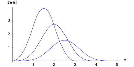
Figure 1: Density of states $\Omega(E)$ given in (5) associated with nondegenerate $(n+1)$-level systems for $n=3,4,5$, with energy eigenvalues $E_{k}=k$ $(k=0,\ldots,n)$. For an $(n+1)$-level system, $\Omega(E)$ is a piecewise polynomial of degree $n-1$, and is $n-2$ times differentiable in energy $E$.

Once the density of states $\Omega(E)$ is obtained for the microcanonical equilibrium, thermal expectation values of physical observables in the corresponding canonical distribution can be computed by use of the canonical partition function $Z(\beta)$, which is the Laplace transform of $\Omega(E)$. When energy eigenvalues are nondegenerate, we have

$$Z(\beta)=\sum_{k=1}^{n+1}{\rm e}^{-\beta E_{k}}\prod_{l=1,\neq k}^{n+1}\frac{\pi}{\beta(E_{l}-E_{k})}.$$ (6)

A line of argument in Khinchin [1] for classical systems can then be applied here in the quantum context to prove that the parameter $\beta$ appearing in (6) for the canonical partition function agrees with the microcanonical definition of temperature in (2).

4 Quantum phase transitions

An interesting consequence of the microcanonical framework, whether classical or quantum, is that the density of states in general need not be an analytic function for finite systems. In contrast, the partition function in the canonical counterpart is necessarily analytic. In other words, while it is necessary in the canonical framework to take thermodynamic limit to describe phase transitions, in the microcanonical formalism this is not the case. Therefore, an approach based on microcanonical equilibrium might provide an adequate description of the phase transitions for small systems observed in the laboratory. We note in this connection that there are many classical systems for which finite-size phase transitions are predicted in microcanonical equilibrium [8, 9].

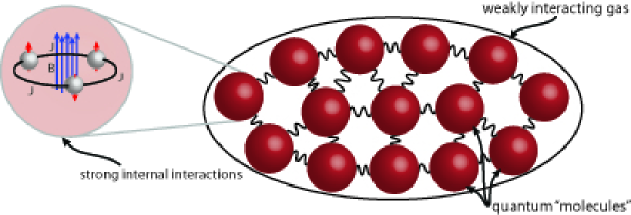
Figure 2: A gas of quantum Ising chains. The gas consists of a large number of weakly interacting quantum molecules. Each molecule is modelled by a quantum Ising chain of three strongly interacting spin-$\textstyle\frac{1}{2}$ particles.

In quantum microcanonical equilibrium, the breakdown of analyticity of $\Omega(E)$ gives rise to phase transitions in the sense that discontinuities in the higher-order derivatives of $\Omega(E)$ emerge. Specifically, if we solve the first equation in (2) for the energy to obtain $E(T)$, then for a system with $n+1$ nondegenerate energy eigenvalues, the $(n-1)$-th derivative of the energy with respect to the temperature has a discontinuity.

As an illustration we consider the specific heat $C(T)$ for a gas of weakly interacting molecules, where each molecule is modelled by a strongly interacting chain of three Ising-type spins (see Figure 2). The molecular Hamiltonian is ${\hat{H}}=-J\sum_{k=1}^{3}\sigma_{z}^{k}\sigma_{z}^{k+1}-B\sum_{k=1}^{3}\sigma_{z}^{k}$, where $\sigma_{z}^{k}$ is the third Pauli matrix for spin $k$, and $J,B$ are constants. For this system, the specific heat grows rapidly in the vicinity of the critical point $T_{c}=(2J+B)/3k_{B}$, where the system exhibits a discontinuity in the second derivative of the specific heat. The plot of the specific heat is shown in Figure 3, along with the corresponding plot for a simple four-level molecular gas; the latter exhibits a second-order phase transition at the critical temperature $k_{B}T_{c}=\mbox{$\textstyle\frac{1}{2}$}\varepsilon$ and critical energy $E_{c}=\varepsilon$, where $\varepsilon$ is the spacing of energy eigenvalues.

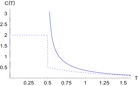
Figure 3: Specific heat for a nondegenerate four-level system (dotted line, $n=3$, $E_{j}=0,1,2,3$), and a quantum Ising chain having a four distinct degenerate eigenvalues (solid line, $J=1/4$, $B=1$). The plots illustrate the existence of second-order phase transitions. In the quantum Ising chain, we have $C(T)\sim(T-T_{c})^{-2}$ away from $T_{c}$, whereas in the vicinity of $T_{c}$ we have $C(T)\sim(T-T_{c})^{-13}$ for $T>T_{c}$.

5 Towards quantum grand microcanonical equilibrium

In the foregoing discussion we have made use of the energy conservation property of the unitary evolution to introduce a quantum microcanonical hypothesis which asserts that in equilibrium, every quantum state with given energy $E$ is realised with an equal probability. This hypothesis can be refined in the following manner, leading to what might appropriately be called the quantum grand microcanonical hypothesis.

For a given quantum mechanical system there are $n$ linearly independent conserved observables, where $n+1$ is the Hilbert space dimensionality. Therefore, when an isolated quantum system with a generic Hamiltonian evolves unitarily, the associated dynamics exhibit ergodicity on the toroidal subspace ${\mathcal{T}}^{n}\subset{\mathcal{E}}_{E}$ of the energy surface determined by simultaneously fixing the expectation values of the commuting family of observables (cf. [10]). A theorem of Birkhoff [1] applies to show that the dynamical average of an observable can be replaced by the ensemble average with respect to a uniform distribution over ${\mathcal{T}}^{n}$. The density of states is then determined by the weighted volume of the subspace ${\mathcal{T}}^{n}$ of the quantum state space.

In the case of the energy observable, the conjugate variable is given by the inverse temperature. For other observables belonging to the commuting family, the associated conjugate variables can be thought of as generalised chemical potentials. In this respect, a refinement of the microcanonical postulate leads to an ensemble of the grand canonical form.

Let us consider the simplest nontrivial example $n=2$. We choose the two projection operators ${\hat{\Pi}}_{1}=|E_{1}\rangle\langle E_{1}|$ and ${\hat{\Pi}}_{2}=|E_{2}\rangle\langle E_{2}|$ for the independent pair of commuting observables. Since these observables are conserved, we let the two constraints be $\langle{\hat{\Pi}}_{1}\rangle=p$ and $\langle{\hat{\Pi}}_{2}\rangle=q$. It follows from the resolution of identity that $\langle{\hat{\Pi}}_{3}\rangle=1-p-q$. In terms of the usual parametrisation, these constraints read $\cos^{2}\mbox{$\textstyle\frac{1}{2}$}\,\theta=p$ and $\sin^{2}\mbox{$\textstyle\frac{1}{2}$}\,\theta\sin^{2}\mbox{$\textstyle\frac{1}{2}$}\,\varphi=q$, respectively. The generalised density of states $\Omega(p,q)=\int_{\Gamma}\delta(\langle{\hat{\Pi}}_{1}\rangle-p)\delta(\langle{\hat{\Pi}}_{2}\rangle-q){\rm d}V_{\Gamma}$ can then be calculated to yield

$$\Omega(p,q)=\mbox{$\textstyle\frac{1}{4}$}\pi^{2}\left(\Upsilon(p)-\Upsilon(p+q-1)\right)\left(\Upsilon(q)-\Upsilon(q-1)\right),$$ (7)

where $\Upsilon(x)=-1$ for $x\leq 0$ and $\Upsilon(x)=1$ for $x>0$. We have $\Omega(p,q)=\pi^{2}$ in the range $0\leq p,q\leq 1$ and $0\leq 1-p-q\leq 1$. To establish its relation with the density of states $\Omega(E)$ we solve the energy constraint $pE_{1}+qE_{2}+(1-p-q)E_{3}=E$ for, say, $p$, then substitute the result in $\Omega(p,q)$, and integrate over $q$ from $0$ to $1$. The temperature of the system can then be obtained by differentiation. It would be of interest to further investigate properties of the grand microcanonical equilibrium for general systems, which in our view holds the promise for many new rigorous results in quantum statistical mechanics.

DCB acknowledges support from The Royal Society. DWH thanks the organisers of the DICE2006 conference in Piombino, Italy, 11-15 September 2006 where this work was presented. The authors thank M. Parry for comments.

References

- [1] A. I. Khinchin, 1949 Mathematical foundations of statistical mechanics (New York: Dover)
- [2] A. Y. Khinchin, 1969 Mathematical foundations of quantum statistics (Toronto: Graylock Press)
- [3] E. Schrödinger 1952 Statistical thermodynamics (Cambridge: Cambridge University Press)
- [4] R. B. Griffiths 1965 Microcanonical ensemble in quantum statistical mechanics. J. Math. Phys. 6 1447-1461
- [5] D. H. E. Gross 2001 Microcanonical Thermodynamics—Phase Transitions in Small Systems, (Singapore: World Scientific)
- [6] M. Schmidt, R. Kusche, W. Kronmüller, B. von Issendorff, & H. Haberland 1997 Experimental determination of the melting point and heat capacity for a free cluster of 139 sodium atoms. Phys. Rev. Lett. 79, 99-102
- [7] D. C. Brody, D. W. Hook, & L. P. Hughston 2005 Quantum phase transitions without thermodynamic limits. quant-ph/0511162
- [8] M. Kastner 2004 Unattainability of a purely topological criterion for the existence of a phase transition for nonconfining potentials Phys. Rev. Lett. 93, 150601
- [9] R. Franzosi & M. Pettini 2004 Theorem on the origin of phase transitions Phys. Rev. Lett. 92, 060601
- [10] D. C. Brody & L. P. Hughston 2001 Geometric quantum mechanics J. Geom. Phys. 38, 19-53