Quantum dynamics of double-qubits in a spin star lattice with an XY interaction

Abstract

The dynamics of two coupled spins-1/2 interacting with a spin-bath via the quantum Heisenberg $XY$ coupling is studied. The pair of central spins served as a quantum open subsystem are initially prepared in two types of states: the product states and the Bell states. The bath, which consists of $N$ (in the thermodynamic limit $N\rightarrow\infty$) mutually coupled spins-1/2, is in a thermal state at the beginning. By the Holstein-Primakoff transformation, the model can be treated effectively as two spin qubits embedded in a single mode cavity. The time-evolution of the purity, z-component summation and the concurrence of the central spins can be determined by a Laguerre polynomial scheme. It is found that (i) at a low temperature, the uncoupled subsystem in a product state can be entangled due to the interaction with bath, which is tested by the Peres-Horodecki separability; however, at a high temperature, the bath produces a stronger destroy effect on the purity and entanglement of the subsystem; (ii) when the coupling strength between the two central spins is large, they are protected strongly against the bath; (iii) when the interaction between the subsystem and the bath is strong, the collapse of the two spin qubits from their initial entangled state is fast.

I Introduction

Compared with other physical systems Braunstein , solid-state devices, in particular, the ultra-small quantum dots Burkard with spin degrees of freedom embedded in nanostructured materials are more easily scaled up to large registers and they can be manipulated by energy bias and tunneling potentials Loss . Naturally, the spin systems are very promising candidates for quantum computation Loss ; Kane ; Nielsen . Inevitably, the spin qubits are open quantum systems Breuer2 ; weiss subjected to the interactions with their environments. In a short time, the states of the qubits will relax into a set of “pointer states” in the Hilbert space Zurek1981 , which can be quantified by using the purity Zurek1987 ; the entanglement between the spin qubits will also vanish. Yet quantum entanglement is the most intriguing feature of quantum composite system and the vital factor for quantum computation and quantum communication Nielsen ; Bennett . These two disadvantages, so-called decoherence and disentanglement, will not be overcome until the modelling of the surrounding environment or bath of the spin systems.

For solid state spin nano-devices, the quantum noise, causing decoherence and disentanglement of the qubits system, mainly arises from the contribution of nuclear spins, which is usually regarded as a spin environment. Recently, there are some works devoted to the behavior of central spins under a strong non-Markovian influence of a spin-bath Stamp ; Loss2 . Lucamarini et al. had used a perturbation method Paganelli and a mean-field approximation Paganelli2 to study the temporal evolution of entanglement pertaining to two qubits interacting with a thermal bath. They found entangled states with an exponential decay of the quantum correlation at finite temperature. Hutton and Bose Hutton investigated a star network of spins, in which all spins interact exclusively and continuously with a central spin via Heisenberg XX couplings with equal strength. Their work was advanced by Hamdouni et al. Hamdouni , who derived the exact reduced dynamics of a central two-qubit subsystem in the same bath configuration. And they also studied the entanglement evolution of the central system. Yuan et al. Yuan developed a novel operator technique to obtain the dynamics of the two coupled spins in quantum Heisenberg XY Breuer spin bath with high symmetry. The results of all the above works are very exciting. Yet all of their methods are of complex analytical derivations. And in Ref. Yuan , their analytical results are dependent on some particular initial states. The study of quantum dynamics from different initial states, such as Bell states and product states, is a very interesting issue in this system. Thus we introduce a “half analytical and half numerical” method here to solve this kind of open quantum problem and show light on their features of dynamics from different initial states. Moreover, the numerical part of our method is beyond the Markovian approximation Fannes due to the strong non-Markovian behavior of such a center-spins-spin-bath model.

In this paper, we study an open two-spin-qubit system in a spin star-like configuration, which is similar to the cases studied in Ref. Yuan ; Hamdouni : the interaction among the bath-spins, between the two qubits and between the subsystem and the bath are all of the Heisenberg XY type. The present model involves the Heisenberg XY interaction that has broad applications for various quantum information processing systems, such as quantum dots, Cavity-QED, etcImamoglu ; Zheng ; Wang ; Lidar . First, we use Holstein-Primakoff transformation to reduce the model to an effective Hamiltonian in the field of cavity quantum electrodynamics Milburn . Second, we apply a numerical simulation to determine the dynamics of the whole system and obtain the reduced dynamics of the two coupled spin qubits by tracing over the bath modes. During our numerical calculation, there are no approximations assumed and the initial state of the subsystem (a pair of central spins) can be chosen arbitrarily. We will give some results about the purity, the z-component summation and the concurrence of the center open spin subsystem in the thermodynamical limit. Additionally, we will show that the bath can lead to entanglement of initially unentangled qubits. The rest of this paper is organized as follows. In Sec. II the model Hamiltonian and the operator transformation procedure is introduced. In Sec. III, we explain the numerical techniques about the evolution of the reduced matrix for the subsystem; Detailed results and discussions are in Sec. IV; The conclusion of our study is given in Sec. V.

II Model and Transformation

Consider a two-spin-qubit subsystem symmetrically interacting with bath spins via a Heisenberg XY interaction: both the subsystem and the bath are composed of spin-1/2 atoms. Each spin in the bath interacts with the two center ones by the same coupling strength, which is similar to the cases in the literatureYuan ; Breuer ; Hutton ; Breuer3 . The interactions between bath spins are also of the XY type. The Hamiltonian for the total system is

$$H = H_{S}+H_{SB}+H_{B}.$$ (1)

$$H_{S} = \mu_{0}(S_{01}^{z}+S_{02}^{z})+\Omega\left(S_{01}^{+}S_{02}^{-}+S_{01}^{-}S_{02}^{+}\right),$$ (2)

$$H_{SB} = \frac{g_{0}}{\sqrt{N}}\left[\left(S_{01}^{+}+S_{02}^{+}\right)\sum_{i=1}^{N}S_{i}^{-}+\left(S_{01}^{-}+S_{02}^{-}\right)\sum_{i=1}^{N}S_{i}^{+}\right],$$ (3)

$$H_{B} = \frac{g}{N}\sum_{i\neq j}^{N}\left(S_{i}^{+}S_{j}^{-}+S_{i}^{-}S_{j}^{+}\right).$$ (4)

Here, $H_{S}$ and $H_{B}$ describe the subsystem and bath respectively, and $H_{SB}$ is the interaction part in the whole Hamiltonian Breuer ; Yuan ; Canosa . $\mu_{0}$ represents the coupling constant between a locally applied external magnetic field along the $z$ direction and the spin qubit subsystem. $\Omega$ is the coupling constant between two qubit spins. $S_{0i}^{+}$ and $S_{0i}^{-}$ ($i$=1,2) are the spin-flip operators of the subsystem qubits, respectively, which are:

$$S^{+}=\left(\begin{array}[]{cc}0&1\\ 0&0\end{array}\right),\quad S^{-}=\left(\begin{array}[]{cc}0&0\\ 1&0\end{array}\right).$$ (5)

$S_{i}^{+}$ and $S_{i}^{-}$ are the corresponding operators for the $i$th atom spin in the bath. The index $i$ in the summation runs from $1$ to $N$, where $N$ is the number of the bath spins. $g_{0}$ is the coupling constant between the subsystem and the bath, and $g$ is the one between any two spins in the bath.

Substituting the collective angular momentum operators $J_{\pm}=\sum_{i=1}^{N}S_{i}^{\pm}$ into Eq. 3, we rewrite the last two parts of the Hamiltonian as:

$$H_{SB} = \frac{g_{0}}{\sqrt{2j}}\left[\left(S_{01}^{+}+S_{02}^{+}\right)J_{-}+\left(S_{01}^{-}+S_{02}^{-}\right)J_{+}\right],$$ (6)

$$H_{B} = \frac{g}{2j}\left(J_{+}J_{-}+J_{-}J_{+}\right)-g,$$ (7)

where $j=N/2$. After the Holstein-Primakoff transformation (It transforms the spin bath of infinity spins into an effective boson bath) Holstein ,

$$J_{+}=b^{+}\left(\sqrt{2j-b^{+}b}\right),\hskip 5.69054ptJ_{-}=\left(\sqrt{2j-b^{+}b}\right)b,$$ (8)

with $[b,b^{+}]=1$, the Hamiltonian, Eqs. 6 and 7, can be written as

$$H_{SB} = g_{0}\left[\left(S_{01}^{+}+S_{02}^{+}\right)\sqrt{1-\frac{b^{+}b}{N}}b+\left(S_{01}^{-}+S_{02}^{-}\right)b^{+}\sqrt{1-\frac{b^{+}b}{N}}\right],$$ (9)

$$H_{B} = g\left[b^{+}\left(1-\frac{b^{+}b}{N}\right)b+\sqrt{1-\frac{b^{+}b}{N}}bb^{+}\sqrt{1-\frac{b^{+}b}{N}}\right]-g.$$ (10)

In the thermodynamic limit (i.e. $N\longrightarrow\infty$) at finite temperatures, we then have

$$H_{SB} = g_{0}\left[\left(S_{01}^{+}+S_{02}^{+}\right)b+\left(S_{01}^{-}+S_{02}^{-}\right)b^{+}\right],$$ (11)

$$H_{B} = 2gb^{+}b.$$ (12)

Although the whole Hamiltonian composed by Eqs. 2, 11 and 12 is similar to that of a Jaynes-Cumming model Yuan , there is an explicit difference between the two models. The present Hamiltonian describes two coupled qubits interacting with a single-mode thermal bosonic bath field, so the analysis of the model is a nontrivial problem in cavity quantum electrodynamics Imamoglu ; Zheng . We note here that due to the transition invariance of the bath spins in our model, it is effectively represented by a single collective environment pseudo-spin $J$ in Eq. 8. After the Holstein-Primakoff transformation and in the thermodynamic limit, this collective environment pseudo-spin could be considered a single-mode bosonic thermal field. The effect of this single-mode environment on the dynamics of the two coupled qubits is interesting and nontrivial. In Sec. IV, we will show some results, for example, the revival behavior of the reduced density matrix and the entanglement evolution of the two central spins. This could be used in real quantum information applications.

III Numerical Calculation procedures

The initial density matrix of the total system is assumed to be separable, i.e., $\rho(0)=|\psi\rangle\langle\psi|\otimes\rho_{B}$. The density matrix of the spin bath satisfies the Boltzmann distribution, that is $\rho_{B}=e^{-H_{B}/T}/Z$, where $Z={\rm Tr}\left(e^{-H_{B}/T}\right)$ is the partition function, and the Boltzmann constant $k_{B}$ has been set to $1$ for sake of simplicity. The density matrix $\rho(t)$ of the whole system can be derived by

$$\rho(t) = \exp(-iHt)\rho(0)\exp(iHt),$$ (13)

$$\rho(0) = \rho_{S}(0)\otimes\rho_{B}(0),$$ (14)

$$\rho_{S}(0) = |\psi(0)\rangle\langle\psi(0)|.$$ (15)

In order to find the density matrix $\rho(t)$, we follow the method suggested by Tessieri and Wilkie TWmodel . The thermal bath state $\rho_{B}(0)$ can be expanded with the eigenstates of the environment Hamiltonian $H_{B}$:

$$\rho_{B}(0) = \sum_{m=1}^{M}|\phi_{m}\rangle\omega_{m}\langle\phi_{m}|,$$ (16)

$$\omega_{m} = \frac{e^{-E_{m}/T}}{Z},$$ (17)

$$Z = \sum_{m=1}^{M}e^{-E_{m}/T}.$$ (18)

Here $|\phi_{m}\rangle$, $m=1,2,3,\cdots,M$, are the eigenstates of $H_{B}$ and $E_{m}$ are the corresponding eigen energies. According to the form of Eq. 12, $|\phi_{m}\rangle=|m\rangle$ and $E_{m}=2gm$, thus $\omega_{m}=\exp(-2gm/T)$ and $Z=1/(1-e^{-2g/T})$. With this expansion, the density matrix $\rho(t)$ can be written as:

$$\rho(t)=\sum_{m=1}^{M}\omega_{m}|\Psi_{m}(t)\rangle\langle\Psi_{m}(t)|.$$ (19)

Where

$$|\Psi_{m}(t)\rangle=\exp(-iHt)|\Psi_{m}(0)\rangle=U(t)|\Psi_{m}(0)\rangle.$$ (20)

The initial state is

$$|\Psi_{m}(0)\rangle=|\psi(0)\rangle|m\rangle.$$

The evolution operator $U(t)$ can be evaluated by different methods. In Ref. Yuan , they use a unique analytical operator technique, which is dependent on the special initial state. Here, we apply an efficient numerical algorithm based on polynomial schemes Jing ; Dobrovitski1 ; Hu into this problem. The method used in this calculation is the Laguerre polynomial expansion method we proposed in Ref. Jing , which is pretty well suited to many quantum systems and can give accurate result with a comparatively smaller computation load. More precisely, the evolution operator $U(t)$ is expanded in terms of the Laguerre polynomial of the Hamiltonian as:

$$U(t)=\left(\frac{1}{1+it}\right)^{\alpha+1}\sum^{\infty}_{k=0}\left(\frac{it}{1+it}\right)^{k}L^{\alpha}_{k}(H),$$

where $\alpha$ distinguishes different types of Laguerre polynomials Arfken ; $k$ is the order of the Laguerre polynomial. In practice, the expansion has to be cut at some value of $k_{\text{max}}$ for the compromise of the numerical stability in the recurrence of the Laguerre polynomial and the speed of calculation. $k_{\text{max}}$ is optimized to be $20$ in this study and the time step $t$ is restricted to some value in order to get accurate results of the evolution operator. At every time step, the accuracy of the results will be confirmed by the test of the numerical stability — whether the trace of the density matrix is $1$ with error less than $10^{-12}$. In a longer time scale, the evolution can be achieved with more steps. The action of the time evolution operator is calculated by utilizing recurrence relations of the Laguerre polynomial. The efficiency of this scheme Jing is about $10$ times as that of the Runge-Kutta algorithm used in Ref. TWmodel . When the states $|\Psi_{m}(t)\rangle$ are obtained, the density matrix can be found by performing the summation in Eq. (19).

In principle we should consider every energy level of the single-mode bath field: $M\rightarrow\infty$. But the contribution of the high energy states $|m\rangle,m>m_{C}$ ($m_{C}$ is a cutoff to the spin bath eigenstates) is found to be negligible due to their weights $\omega_{m}$ as long as the temperature is finite. That is to say, Eq. (19) could be changed to the following form:

$$\rho(t)=\sum_{m=1}^{m_{C}}\omega_{m}|\Psi_{m}(t)\rangle\langle\Psi_{m}(t)|.$$ (21)

Given the density matrix of the whole system $\rho(t)$, we can find the reduced density matrix by a partial trace operation, which traces out the freedom degrees of the environment:

$$\rho_{S}(t)={\rm Tr}_{B}\left(\rho(t)\right).$$ (22)

For our model, $\rho_{S}=|\psi\rangle\langle\psi|$ is a density matrix of the open subsystem consists of two coupled central spins, which can be expressed by a $4\times 4$ matrix in the subsystem Hilbert space spanned by the orthonormal vectors $|00\rangle$, $|01\rangle$, $|10\rangle$ and $|11\rangle$. The most general form of an initial pure state of the two-qubit system is

$$|\psi(0)\rangle=\alpha|00\rangle+\beta|11\rangle+\gamma|01\rangle+\delta|10\rangle,$$ (23)

$$\mbox{with}\quad|\alpha|^{2}+|\beta|^{2}+|\gamma|^{2}+|\delta|^{2}=1.$$ (24)

IV Numerical simulation results and discussions

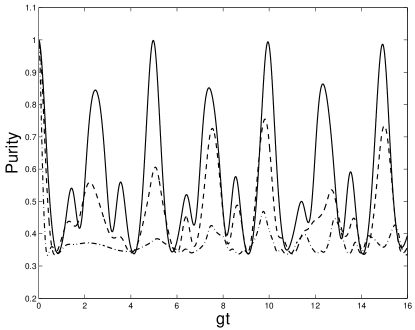
(a) Purity

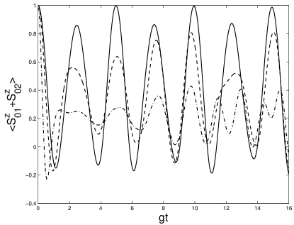
(b) $\langle{}S^{z}_{01}+S^{z}_{02}\rangle$

Figure 1: Time evolution of (a) purity and (b) z-component oscillation for an initial two-qubit state of $|\psi(0)\rangle=|11\rangle$ for different values temperature: $T=0.2g$ (solid curve), $T=2g$ (dashed curve) and $T=10g$ (dot dashed curve). Other parameters are $\mu_{0}=2g$, $g_{0}=g$, $\Omega=0g$.

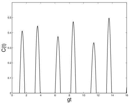
Figure 2: Time evolution of the concurrence for an initial two-qubit state of $|\psi(0)\rangle=|11\rangle$ at low temperature: $T=0.2g$. Other parameters are $\mu_{0}=2g$, $g_{0}=g$, $\Omega=0g$.

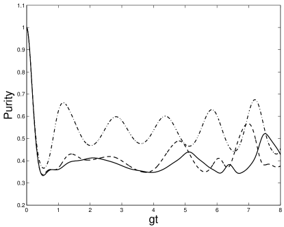
(a) Purity

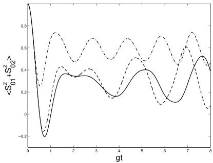
(b) $\langle{}S^{z}_{01}+S^{z}_{02}\rangle$

Figure 3: Time evolution of (a) purity and (b) z-component oscillation for an initial two-qubit state of $|\psi(0)\rangle=|11\rangle$ for different values $\Omega$: $\Omega=0g$ (solid curve), $\Omega=2g$ (dashed curve) and $\Omega=5g$ (dot dashed curve). Other parameters are $\mu_{0}=2g$, $g_{0}=g$, $T=5g$.

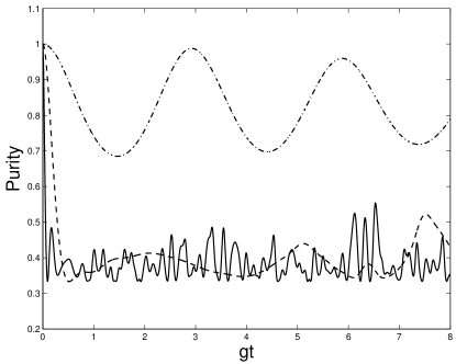
(a) Purity

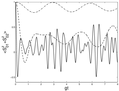
(b) $\langle{}S^{z}_{01}+S^{z}_{02}\rangle$

Figure 4: Time evolution of (a) purity and (b) z-component oscillation for an initial two-qubit state of $|\psi(0)\rangle=|11\rangle$ for different values $g_{0}$: $g_{0}=0.2g$ (dot dashed curve), $g_{0}=g$ (dashed curve) and $g_{0}=5g$ (solid curve). Other parameters are $\mu_{0}=2g$, $\Omega=0g$, $T=5g$.

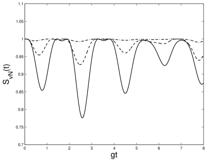
(a) $S_{vN}(t)$

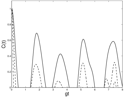
(b) $C(t)$

Figure 5: Time evolution of (a) von Neumann entropy and (b) Concurrence for an initial two-qubit state of $|\psi(0)\rangle=1/\sqrt{2}(|01\rangle+|10\rangle)$ for different values temperature: $T=2g$ (solid curve), $T=5g$ (dashed curve) and $T=20g$ (dot dashed curve). Other parameters are $\mu_{0}=2g$, $g_{0}=g$, $\Omega=0g$.

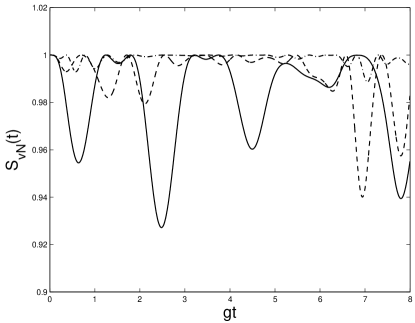
(a) $S_{vN}(t)$

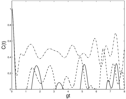
(b) $C(t)$

Figure 6: Time evolution of (a) von Neumann entropy and (b) Concurrence for an initial two-qubit state of $|\psi(0)\rangle=1/\sqrt{2}(|01\rangle+|10\rangle)$ for different values $\Omega$: $\Omega=0g$ (solid curve), $\Omega=2g$ (dashed curve) and $\Omega=5g$ (dot dashed curve). Other parameters are $\mu_{0}=2g$, $g_{0}=g$, $T=5g$.

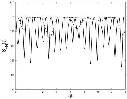
(a) $S_{vN}(t)$

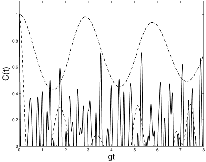
(b) $C(t)$

Figure 7: Time evolution of (a) von Neumann entropy and (b) Concurrence for an initial two-qubit state of $|\psi(0)\rangle=1/\sqrt{2}(|01\rangle+|10\rangle)$ for different values $g_{0}$: $g_{0}=0.2g$ (dot dashed curve), $g_{0}=g$ (dashed curve) and $g_{0}=5g$ (solid curve). Other parameters are $\mu_{0}=2g$, $\Omega=0g$, $T=5g$.

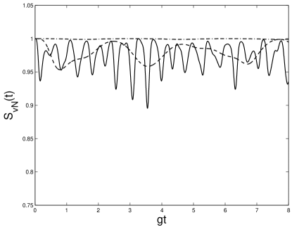
(a) $S_{vN}(t)$

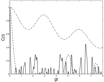
(b) $C(t)$

Figure 8: Time evolution of (a) von Neumann entropy and (b) Concurrence for an initial two-qubit state of $|\psi(0)\rangle=1/\sqrt{2}(|00\rangle+|11\rangle)$ for different values $g_{0}$: $g_{0}=0.2g$ (dot dashed curve), $g_{0}=g$ (dashed curve) and $g_{0}=5g$(solid curve). Other parameters are $\mu_{0}=2g$, $\Omega=0g$, $T=5g$.

After we obtain the reduced density matrix, we can calculate any physical quantities of the subsystem. In the following we focus our attention on three important physical quantities of the subsystem which reflect the quantum entropy increase caused by decoherence, the population inversion and the entanglement degree of the subsystem state respectively. These quantities are (i) the time dependence of the state purity, i.e. $P={\rm Tr}(\rho_{S}^{2})$, which characterizes the conservation of the purity of the subsystem Zurek1987 ; Zurek1981 . If $P=1$, the subsystem is a pure state; whereas $P=1/2^{n}$ (considering there are $n$ spins-1/2 in the subsystem), it is in a completely mixed state $\rho_{S}=1/2^{n}I$ ($I$ is the identical matrix in $2^{n}$ dimension). (ii) the $z$-component of the central spins, i.e. $\langle{}S^{z}_{01}+S^{z}_{02}\rangle$, which demonstrates the population probability of the system. (iii) the time-evolution of concurrence Wootters1 ; Wootters2 for the two central spins of the open subsystem. The concurrence of the two spin-1/2 system is an indicator of their intra entanglement, which is defined as Wootters1 :

$$C=\max\{\lambda_{1}-\lambda_{2}-\lambda_{3}-\lambda_{4},~{}0\},$$ (25)

where $\lambda_{i}$ are the square roots of the eigenvalues of the product matrix $\rho_{S}(\sigma^{y}\otimes\sigma^{y})\rho^{*}_{S}(\sigma^{y}\otimes\sigma^{y})$ in decreasing order.

Theoretically, our method can deal with time evolution of the subsystem from any initial state. Here we first discuss the case of $|\psi(0)\rangle=|11\rangle$, which means both of the two center spins are in their excited states. The time evolution of the purity at different temperatures is given in Fig. 1(a) as well as the expecting value of the z-component in Fig. 1(b). We find that, (i) at a very low temperature, both the quantities present a collapse and revival phenomenon, which is identical with the two photons resonance of two two-level atoms in a cavity. In Fig. 1(a), the state of the first peak point ($gt_{1}=1.424$) along the solid line is

$$\rho_{S}(gt_{1})=0.1472|11\rangle\langle 11|+0.1472|00\rangle\langle 00|+0.7056|B\rangle\langle{}B|,$$

where $|B\rangle=1/\sqrt{2}(|01\rangle+|10\rangle)$. By the Peres-Horodecki separability Horodecki test, and if we make a positive partial transposition (PPT) operation to the $1$st center spin, we will get a new matrix:

$$\rho_{S}^{T_{1}}(gt_{1})=0.1472|11\rangle\langle 11|+0.1472|00\rangle\langle 00|+0.3528(|10\rangle\langle 10|+|01\rangle\langle 01|+|11\rangle\langle 00|+|00\rangle\langle 11|),$$

whose spectrum is $\{0.500,0.3528,0.3628,-0.2055\}$. It shows explicitly that the bath can entangle the subsystem spins, although they are separable initially. And the state of the second peak point ($gt_{2}=2.468$) is

$$\rho_{S}(gt_{2})=0.9169|11\rangle\langle 11|+0.0574|00\rangle\langle 00|+0.02574|B\rangle\langle{}B|,$$

which could be approximated as its start state $|11\rangle\langle 11|$. In fact, one can find the time evolution of the subsystem concurrence in the condition of $|\psi(0)\rangle=|11\rangle$ and $T=0.2g$ in Fig. 2. It is interesting that the bath can induce entanglement between the two central spins periodically even without the direct coupling between the two spins. The peak state ($t_{2}=4.972g$) (the solid line in Fig. 1(a))is

$$\rho_{S}(t_{2})=0.9992|11\rangle\langle 11|+0.0008|00\rangle\langle 00|+0.00002|B\rangle\langle{}B|,$$

which could be approximated as its initial state $|11\rangle\langle 11|$. Then the subsystem revives at this time point and the period of the revival is about $5g$. (ii) with increasing temperature, their oscillation magnitudes are quickly damped by the thermal bath: For the purity at $T=10g$, $P\rightarrow 0.3$ means a much large derivation from the initial state (to see the dot dashed curve in Fig. 1(a)); For the z-component summation of the two spins, it means the degeneration of their magnetization (to see the dot dashed curve in Fig. 1(b)). Then we hold the bath at a moderate temperature $T=5g$ to research the role of the direct coupling between the two central spins. In Fig. 3(a), with increasing $\Omega$, the correlation between the two spins is strengthened so that the leakage of the information in the open subsystem is reduced and the collapse speed of the subsystem state slows down and distinct revivals are observed. In Fig. 3(b), the whole magnetic moment oscillates around a mean value $\langle{}S^{z}_{01}+S^{z}_{02}\rangle=0.6$ when $\Omega$ is as large as $5g$. One can see that if the direct coupling between the two central spins is strong enough, the two qubits can keep their initial state from the influence of the bath. The effect of the coupling strength between the qubit subsystem spins and bath spins $g_{0}$ can be found in Fig. 4. At a large value $g_{0}=5g$, the strong interaction with the bath will quickly push the pure state of the subsystem into a mixed state (to see the solid curve in Fig. 4(a)); on the contrary, at a small value $g_{0}=0.2g$, the initial state can be conserved to a great extent, $P>0.68$, as the dot dashed curve shows in Fig. 4(b).

Then we show the results of the temporal evolution for the quantum entropy and concurrence from a most entangled state (one of the well-known Bell states) $|\psi(0)\rangle=1/\sqrt{2}(|01\rangle+|10\rangle)$ under the influence of the bath. As is known, the entropy of either particle inside a Bell states is $1$, which is certainly in a most mixed state. On one hand, in Fig. 5(a), at any finite temperature, the entropy will return $1$ after some fluctuation; on the other hand, in Fig. 5(b), the entanglement degree between the two coupled spins will quickly collapse to zero and make some fluctuations and revivals accidently. The magnitudes of these fluctuations decrease with increasing temperature in both figures. The damping speed of concurrence evidently increases with temperature in Fig. 5(b) and when $T=20g$, it shows a sudden death in a much short time and a tiny revival in a long time scale. In Fig. 6(a), the effect of subsystem inner-coupling $\Omega$ on the entropy is so weak that the biggest fluctuation of that is less than $0.08$ and when $\Omega=5g$, this effect can be neglected. Yet, in Fig. 6(b), the concurrence can be restored to some extent with a comparatively larger $\Omega$: when $\Omega=5g$, there is no sudden death of the entanglement between the subsystem spins and the concurrence oscillates about $C=0.4$. From the above results, we find that the von-Neumann entropy is not a very good measure of this subsystem (consisted of two or more atoms) state as concurrence. In Fig. 7, with decreasing interaction between the open subsystem and the bath $g_{0}$, the influence of the bath spins on the subsystem is reduced. As is depicted in Fig. 7(b), at $g_{0}=0.2g$, the dot dashed line oscillates around the $C=0.7$. This is evident that if we can keep the coupling between the subsystem and the bath as weak as possible, then the entanglement of subsystem can be conserved as much as possible.

With the combination of the technique of Holstein-Primakoff operator and our polynomial numerical scheme, we have thoroughly discussed the quantum dynamics of two central spins in a spin star lattice within XY interaction from different kinds of initial states. In principle, all the physical quantities can be calculated as the above ones. For the product states, it is noticed that the bath can help to entangle the two separable spins; For the Bell states, it is valuable that $g_{0}$, the interaction between the subsystem and environment, can be adjusted to slower the collapse of the most entangled state. However, we also find that the behavior of the reduced density matrix for the open subsystem relies on different initial state although they are all of the Bell states. By the comparison of Fig. 7 with Fig. 8, it is shown: in the former figure, when $g_{0}$ is small, the concurrence can be maintained for a long time; while in the latter one, when $g_{0}$ is enhanced, it is quickly damped.

V Conclusion

We have studied the quantum dynamics of the purity, z-component summation and concurrence of two coupled spin qubits in a apin bath via Heisenberg $XY$ interaction. A novel numerical polynomial scheme is used in the calculation for the reduced density matrix of the central qubits after the model Hamiltonian has been performed by the well-known Holstein-Primakoff transformation. The procedure avoids the difficulty in Ref. Yuan that the initial state is limited by the analytic derivation. The time evolution of different types of initial states, either product states or Bell ones, is obtained. Although the subsystem is initially prepared in the product state ($|11\rangle$) , it turns out that the bath can induce entanglement on the subsystem spins by the Peres-Horodecki separability test on the state $\rho_{S}^{T_{1}}(gt_{1})$. On the other hand, the effect of different types of coupling on the entanglement of the system is studied. Generally, the coupling to the environment reduces the initial state entanglement. When the interaction between the two spins is large, they are protected strongly against the environment. Thus, it is found that the dynamics of the subsystem depends sensitively on the initial state, the bath temperature, the inner-coupling between the two central spins and the interaction between the subsystem and the environment. Besides, our numerical scheme is simple and independent of the initial state, which can be easily applied to the studies of some other kinds of open quantum systems.

- (1) S. Braunstein, and H. K. Lo, Eds., Fortschr. Phys. 48, 765 (2000).
- (2) G. Burkard, D. Loss and D. P. DiVincenzo, Phys. Rev. B 59, 2070 (1999).
- (3) D. Loss, and D. P. DiVincenzo, Phys. Rev. A 57, 120 (1998).
- (4) B. E. Kane, Nature (London) 393, 133 (1998).
- (5) M. A. Nielsen and I. L. Chuang, Quantum Computation and Quantum Information (Cambridge University Press, Cambridge, 2000).
- (6) H. P. Breuer and F. Petruccione, The Theory of Open Quantum Systems (Oxford University Press, Oxford, 2002).
- (7) U. Weiss, Quantum Dissipative Systems, (World Scientific, 2nd ed) (1999).
- (8) W. H. Zurek, Phys. Rev. D, 24, 1516 (1981).
- (9) W. H. Zurek, S. Habib and J. P. Paz, Phys. Rev. Lett., 70, 1187 (1987)
- (10) C. H. Bennett, H. J. Bernstein, S. Popescu, B. Schumacher, Phys. Rev. A 53, 2046 (1996).
- (11) N. V. Prokof er and P. C. E. Stamp, Rep. Prog. Phys. 63, 669 (2000).
- (12) J. Schliemann, A. Khaetskii, and D. Loss, J. Phys.: Con- dens Matter 15, R1809 (2003).
- (13) S. Paganelli, F. de Pasquale, and S. M. Giampaolo, Phys. Rev. A 66, 052317 (2002).
- (14) M. Lucamarini, S. Paganelli, and S. Mancini, Phys. Rev. A 69, 062308 (2004).
- (15) A. Hutton and S. Bose, Phys. Rev. A 69, 042312 (2004).
- (16) Y. Hamdouni, M. Fannes, and F. Petruccione, Phys. Rev. B 73, 245323 (2006).
- (17) X.Z. Yuan, H. Goan, and K.D. Zhu, Phys. Rev. B 75, 045331 (2007).
- (18) H. P. Breuer, D. Burgarth, and F. Petruccione, Phys. Rev. B, 70, 045323 (2004).
- (19) Y. Hamdouni, M. Fannes, and F. Petruccione, Phys. Rev. B, 73, 245323 (2006).
- (20) A. Imamoglu, D. D. Awschalom, G. Burkard, D. P. Di- Vincenzo, D. Loss, M. Sherwin, and A. Small, Phys. Rev. Lett. 83, 4204 (1999).
- (21) S. B. Zheng and G. C. Guo, Phys. Rev. Lett. Phys. 85, 2392 (2000).
- (22) X. Wang, Phys. Rev. A 64, 012313 (2001).
- (23) D. A. Lidar and L. A. Wu, Phys. Rev. Lett.88, 017905 (2002).
- (24) M. Sarovar, H. S. Goan, T. P. Spiller, and G. J. Milburn, Phys. Rev. A 72, 062327 (2005).
- (25) H. P. Breuer, Phys. Rev. A 69, 022115 (2004).
- (26) N. Canosa and R. Rossignoli, Phys. Rev. A 73, 022347 (2006).
- (27) T. Holstein and H. Primakoff, Phys. Rev. 58, 1098 (1949).
- (28) J. Jing and H. R. Ma, Phys. Rev. E 75, 016701 (2007) (2006).
- (29) V. V. Dobrovitski and H. A. De Raedt, Phys. Rev. E 67, 056702 (2003).
- (30) X. G. Hu, Phys. Rev. E, 59, 2471 (1999).
- (31) G. Arfken Mathematical Methods of Physicists, New York: Academic, 3rd ed, (1985).
- (32) L. Tessieri and J. Wilkie, J. Phys. A, 36, 12305 (2003).
- (33) S. Hill and W. K. Wootters, Phys. Rev. Lett. 78, 5022 (1997).
- (34) W. K. Wootters, Phys. Rev. Lett. 80, 2245 (1998).
- (35) M. Horodecki, et al. Phys. Rev. A, 59, 4206 (1999).