Quantum fluctuations of Coulomb Potential as a Source of Flicker Noise. The Influence of Heat Bath

Abstract

The power spectrum of finite-temperature quantum electromagnetic fluctuations produced by elementary charge carriers under the influence of external electric field is investigated. It is found that under the combined action of the photon heat bath and the external field, the low-frequency asymptotic of the power spectrum is modified both qualitatively and quantitatively. The new term in the power spectrum is inversely proportional to frequency, but is odd with respect to it. It comes from the connected part of the correlation function, and is related to the temperature and external field corrections to the photon and charge carrier propagators. In application to the case of a biased conducting sample, this term gives rise to a contribution to the voltage power spectrum which is proportional to the absolute system temperature, the charge carrier mobility, the bias voltage squared, and a factor describing dependence of the noise intensity on the sample geometry. It is verified that the derived expression is in agreement with the experimental data on $1/f$-noise measurements in metal films. It is shown also that the obtained result provides a natural resolution to the problem of divergence of the total noise power.

I Introduction

The origin of flicker noise buck observed in virtually all conducting media remains an open issue in condensed matter theory. Despite numerous models suggested since its discovery eighty years ago there is presently no consistent theory which would explain the main characteristic properties of this omnipresent noise. The power spectral density of flicker noise is proportional to $f^{-\gamma},$ where $f$ is frequency, and the exponent $\gamma$ is about unity (usually $\gamma$ takes values $0.9$ to $1.5$). One of the essential difficulties for theoretical explanation is the fact that experiments show no limits for this dispersion law, neither lower or upper. Although flicker noise dominates only at sufficiently low frequencies, the $1/f$-component is detected in the whole measured band up to $10^{6}{\rm Hz}.$ It is also experimentally established that the noise power spectrum of a sample is proportional to the applied bias squared, and roughly inversely proportional to its volume.

Ubiquity of flicker noise and universality of its properties suggest existence of a simple reason for its occurrence. It is natural to expect this reason to have a quantum origin. Although some of the models suggested so far do consider various quantum effects as underlying mechanisms of flicker noise (such as, for instance, trapping of charge carriers), it may well be that its origin is to be sought at the most fundamental level. Namely, it is plausible that the phenomenon of flicker noise has its roots in the very quantum nature of interaction of elementary charges with electromagnetic field. From this point of view, the problem was attacked by Handel handel1 , who suggested that the observed flicker noise is related to the spectrum of low-energy photons emitted in any scattering process, which, according to Handel, has the $1/f$ profile and reflects the well-know property of bremsstrahlung, namely, the infrared divergence of the cross-section considered as a function of the energy loss. Later, the argument was modified and the so-called coherent quantum $1/f$ effect described handel2 on the basis of quantum electrodynamic results of Kibble and Zwanziger zwan ; kibble . Although Handel’s theory was severely criticized in many respects tremblay ; kampen , it has found support in independent investigations of Refs. vliet ; ziel . Handel’s approach is based on consideration of current fluctuations. An essentially different quantum approach to the problem was recently proposed kazakov1 ; kazakov2 , in which flicker noise is treated as a voltage fluctuation originating from quantum fluctuations of individual electric fields of charge carriers. In this case, the noise power spectrum is found by evaluating the two-point correlation function of the Coulomb potential of an elementary particle, dispersion of this function being related to the quantum spreading of the particle wave packet. However, the magnitude of noise induced by an external electric field, given by this theory, turned out to be too small to explain the observed noise level.

The purpose of this paper is to show that the value of induced quantum noise is actually significantly higher than the previously calculated. It turns out that in evaluating the effect of external electric field it is essential to take into account statistical properties of electromagnetic field. The point is that simultaneous account of the effects of photon heat bath and external field leads to appearance of a contribution of new type. Namely, the new term in the noise power spectrum is odd with respect to frequency, and hence corresponds to the part of the correlation function, which is odd with respect to the difference of its time arguments. The underlying reason that makes the appearance of this term possible is the inhomogeneity in time of fluctuations produced by individual charge carriers. As a consequence of this inhomogeneity, the correlation function of each individual contribution to the Coulomb field fluctuation depends on both time arguments separately, rather than on their difference only, so that symmetry under interchanging of the arguments does not forbid appearance of the odd contribution. The time homogeneity is restored only after summing up all independent contributions. The new contribution stems from the connected part of the correlation function of particle’s field, rather than from the disconnected one that was in focus of Ref. kazakov2 , and is related to the temperature and external field corrections to the photon and charge carrier propagators, in contrast to considerations of Ref. kazakov2 where thermal bath and external field affected only real particle states.

The paper is organized as follows. In Sec. II.1 we briefly discuss the role of the heat bath effects in evaluating the mean value and the correlation function of electromagnetic field produced by elementary particles, and identify the contributions relevant in the low-frequency regime. The power spectral functions of the Coulomb field and voltage fluctuations are defined in Sec. II.2, and written in the form convenient for explicit calculations which are carried out in Sec. III. The low-frequency asymptotic of the power spectrum of Coulomb potential fluctuations in the absence of external electric field is evaluated in Sec. III.1, and is found to exhibit an inverse frequency dependence. However, the $1/f$ part of the spectrum is cancelled in the expression for the voltage spectral density. The non-vanishing $1/f$-contribution to the voltage power spectrum is obtained in Sec. III.2 upon account of the influence of external homogeneous electric field on the virtual charger particle propagation. Application of the obtained results to solids and comparison with experimental data is given in Sec. III.4. Gauge independence of our treatment of electromagnetic fluctuations is proved in the Appendix.

II Preliminaries

II.1 Heat bath contribution to particle propagators

Consider a quantized system of charged particles interacting with electromagnetic field. Let $T$ be the absolute temperature of the system. We are interested in the influence of finite temperature on quantum properties of the electromagnetic field produced by charged particles. Specifically, finite-temperature correlations in the values of the particle’s Coulomb fields will be investigated. To the leading order in the electromagnetic coupling, these correlations are a single-particle effect, in the sense that in this case only fields produced by one and the same particle correlate. In what follows, we thus confine ourselves to systems which allow perturbative treatment of charge carrier collisions, either in terms of original particles, or in terms of quasi-particles (e.g., conduction electrons in metals). In the latter case, the particle’s mass and energy-momentum relation should be replaced by the effective ones.

In this section, we shall discuss some general features of the temperature effect, related to the heat bath influence on virtual propagation of the electromagnetic and charged field quanta. Evidently, the heat bath has no effect on the mean electromagnetic field of a charged particle. Indeed, under above assumptions, this field can be represented as the amplitude of one-photon emission in a transition between free charged particle states, contracted with the photon propagator. Since the 4-vector of momentum transfer to a free massive particle, $p,$ is always spacelike, $p^{2}<0,$ distribution of real photons appearing in the definition of the photon propagator is immaterial in the calculation of the field. As a consequence, quantities built from the mean field, such as the disconnected part of the correlation function, are not affected by the photon heat bath (details of evaluation of this part see in Refs. kazakov1 ; kazakov2 ). Things change, however, when the connected part of the two-point correlation function of electric potential is considered. It is defined by the following symmetric expression

$$C^{\rm con}_{00}(x;x^{\prime})=\frac{1}{2}\langle{\rm in}|\hat{A}_{0}(x)\hat{A}_{0}(x^{\prime})+\hat{A}_{0}(x^{\prime})\hat{A}_{0}(x)|{\rm in}\rangle\,,$$ (1)

where $x$ and $x^{\prime}$ are the spacetime coordinates of two observation points, $\hat{A}_{0}$ is the scalar potential Heisenberg operator, and $|{\rm in}\rangle$ denotes the given in state of the system “charged particle + electromagnetic field.” In the two-photon processes, photon momenta are allowed to take on lightlike directions, and hence the photon heat bath does contribute to the function $C^{\rm con}_{00}(x;x^{\prime}).$

As is well-known, the ordinary Feynman rules of the S-matrix theory are not generally applicable for the calculation of in-in expectation values, and must be modified, e.g., according to Schwinger and Keldysh keldysh . This complication was overcome in kazakov2 by rewriting Eq. (1) in the form

$$C^{\rm con}_{00}(x;x^{\prime})={\rm Re}\langle{\rm out}|T\{\hat{A}_{0}(x)\hat{A}_{0}(x^{\prime})\}|{\rm in}\rangle\,,$$ (2)

which allows the use of the S-matrix rules. This transformation uses equivalence of the one-particle in and out states (and Hermiticity of the electromagnetic field operator). It is applicable to the present case as well, despite the fact that now the in state is not one-particle, because we are not going to take into account scattering processes in the heat bath itself. This can also be shown directly at the diagrammatic level following the route of transformations taken in Ref. kazakov , which is formally the same in zero- and nonzero-temperature cases. Thus, in order to calculate the in-in expectation value (1) taking into account the heat bath effect, the standard finite-temperature-field-theory techniques can be used landsman . Below we employ a version of the real time formalism, developed in niemi , which is especially convenient in actual calculations since the momentum space propagators in this formulation do not involve the step function.

The real time formulation involves doubling of all fields, which will be specified by a two-valued lower index. According to the diagrammatic rules derived in niemi , the photon propagator has the following matrix structure

$$\mathfrak{D}_{\mu\nu}(x) = \int\frac{d^{4}k}{(2\pi)^{4}}\mathfrak{D}_{\mu\nu}(k)e^{-ikx}\,,\quad\mathfrak{D}_{\mu\nu}(k)=4\pi\eta_{\mu\nu}\left(\begin{array}[]{cc}D_{11}(k)&D_{12}(k)\\ D_{21}(k)&D_{22}(k)\end{array}\right)\,,$$ (5)

where

$$D_{11}(k)=-D^{*}_{22}(k)=\frac{1}{k^{2}+i0}-\frac{2\pi i\delta(k^{2})}{e^{\beta|k_{0}|}-1}\,,\quad D_{12}(k)=D_{21}(k)=-\frac{2\pi i\delta(k^{2})e^{\beta|k_{0}|/2}}{e^{\beta|k_{0}|}-1}\,,$$

$\beta=1/T$ being the inverse absolute temperature of the system. In applications to the problem of $1/f$-noise considered below, the value of the product $\beta|k_{0}|$ turns out to be very small. For instance, even for frequencies as large as $10^{6}{\rm Hz},$ and temperatures as small as $1^{\circ}{\rm K},$ it is less than $10^{-27}\cdot 10^{6}/(10^{-16})=10^{-5}$ (the factors $10^{-27}$ and $10^{-16}$ are contributed by the Planck and Boltzmann constants, respectively), so the denominators in the above expressions can be replaced by $\beta|k_{0}|,$ implying that the second term in $D_{11}$ dominates. On the other hand, the temperature effect on the propagation of massive particles is much less prominent. For instance, in the case of conduction electrons in a crystal (this case will be used throughout as a standard example), the particle energy $\varepsilon$ is of the order $(\hbar/d)^{2}/m,$ where $m$ is the particle mass, and $d$ is the lattice spacing. Taking $d\sim 10^{-8}{\rm cm},$ $m\sim 10^{-27}{\rm g},$ we find that $\varepsilon/T\sim 10^{+5},$ so that the temperature contributions can be completely neglected (for fermions as well as for bosons), and the propagator taken in the simple diagonal form

$$\mathfrak{D}^{\phi}(x) = \int\frac{d^{4}k}{(2\pi)^{4}}\mathfrak{D}^{\phi}(k)e^{-ikx}\,,\quad\mathfrak{D}^{\phi}(k)=\left(\begin{array}[]{cc}D^{\phi}_{11}(k)&0\\ 0&D^{\phi}_{22}(k)\end{array}\right)\,,$$ (8)

$$D^{\phi}_{11}(k) = -D^{\phi*}_{22}(k)=(m^{2}-k^{2}-i0)^{-1}\,.$$

This is for a scalar particle described by the action

$$S_{\phi} = {\displaystyle\int}d^{4}x\left\{(\partial_{\mu}\phi^{*}+ieA_{\mu}\phi^{*})(\partial^{\mu}\phi-ieA^{\mu}\phi)-m^{2}\phi^{*}\phi\right\}\,,$$ (9)

where $e$ is the particle charge. Account of particle spin, though adds some extra algebra, does not change the long-range properties of its field, so that following Ref. kazakov2 we work with the simplest case of zero-spin particles. The matrix propagators are multiplied in the interaction vertices, generated by the triple and higher order terms in the Lagrangian, with an additional minus sign for the product of 2-components, as in the Schwinger-Keldysh techniques. The arguments of the Green functions are treated as 1-component fields. Finally, external particle lines represent normalized particle amplitudes or their conjugates, according to whether the particle is incoming or outgoing, just like in the conventional techniques.

As was mentioned above, the photon propagator is dominated by the temperature contribution (as long as the range of momentum integration contains lightlike directions, see discussion in Sec. III.1), while in the massive particle propagator this contribution is negligible. It is important, on the other hand, that the heat bath affects significantly the real particle propagation, i.e., external matter lines in the diagrams. Bilinears of the particle amplitudes representing these lines are expressed eventually via statistical distribution function (see Sec. III.2 for details). Thus, apart from explicit $T$-dependence coming from the photon propagator, the correlation function also depends on temperature implicitly through the particle statistical distribution.

II.2 Power spectral densities of potential and voltage fluctuations

Connected contribution to the power spectral density of electric potential fluctuations is obtained by Fourier transforming Eq. (1) with respect to the difference of the time instants $t,t^{\prime}$:

$$C(\bm{x},\bm{x}^{\prime},t^{\prime},\omega)=\int\limits_{-\infty}^{+\infty}d\tau C^{\rm con}_{00}(\bm{x},t^{\prime}+\tau;\bm{x}^{\prime},t^{\prime})e^{-i\omega\tau}\,.$$ (10)

The upper and lower indices in the notation of the correlation function are suppressed in the left hand side, for brevity. We are interested ultimately in the power spectrum of voltage fluctuations, $C_{U},$ measured between two observation points $\bm{x},\bm{x}^{\prime}$ (e.g., two leads attached to a conducting sample). The connected contribution to the voltage correlation function is given by

$$C_{U}(\bm{x},\bm{x}^{\prime},t,t^{\prime})=\frac{1}{2}\langle{\rm in}|\hat{U}(t)\hat{U}(t^{\prime})+\hat{U}(t^{\prime})\hat{U}(t)|{\rm in}\rangle\,,$$ (11)

where $\hat{U}(t)=\hat{A}_{0}(\bm{x},t)-\hat{A}_{0}(\bm{x}^{\prime},t)$ is the operator of voltage between the two points. This function is separately symmetric with respect to the interchanges $\bm{x}\leftrightarrow\bm{x}^{\prime},$ and $t\leftrightarrow t^{\prime},$ unlike the function $C^{\rm con}_{00}(x;x^{\prime})$ which is only symmetric under $x\leftrightarrow x^{\prime}.$ Substituting the definition of $\hat{U}(t)$ in Eq. (11), the former can be expressed via the latter

$$C_{U}(\bm{x},\bm{x}^{\prime},t,t^{\prime}) = C^{\rm con}_{00}(\bm{x},t;\bm{x},t^{\prime})+C^{\rm con}_{00}(\bm{x}^{\prime},t;\bm{x}^{\prime},t^{\prime})$$ (12)

$$- \left[C^{\rm con}_{00}(\bm{x},t;\bm{x}^{\prime},t^{\prime})+C^{\rm con}_{00}(\bm{x}^{\prime},t;\bm{x},t^{\prime})\right]\,.$$

Accordingly, the power spectral density of voltage fluctuations, defined by

$$C_{U}(\bm{x},\bm{x}^{\prime},t^{\prime},\omega)=\int\limits_{-\infty}^{+\infty}d\tau C_{U}(\bm{x},t^{\prime}+\tau,\bm{x}^{\prime},t^{\prime})e^{-i\omega\tau}\,,$$ (13)

is expressed through that of potential fluctuations as

$$C_{U}(\bm{x},\bm{x}^{\prime},t^{\prime},\omega) = C(\bm{x},\bm{x},t^{\prime},\omega)+C(\bm{x}^{\prime},\bm{x}^{\prime},t^{\prime},\omega)-\left[C(\bm{x},\bm{x}^{\prime},t^{\prime},\omega)+C(\bm{x}^{\prime},\bm{x},t^{\prime},\omega)\right]\,.$$ (14)

Although $C_{U}(\bm{x},\bm{x}^{\prime},t,t^{\prime})$ is symmetric with respect to the interchange $t\leftrightarrow t^{\prime},$ it depends on both time arguments separately, and therefore $C_{U}(\bm{x},\bm{x}^{\prime},t,\omega)$ does not have to be an even function of $\omega.$

When calculating the power spectrum of potential fluctuations according to Eqs. (2), (10), it is convenient to perform the Fourier transformation under the sign “Re” in Eq. (2). For this purpose we introduce the Fourier transform of the two-point Green function:

$$G(\bm{x},\bm{x}^{\prime},t^{\prime},\omega)=\int\limits_{-\infty}^{+\infty}d\tau G(\bm{x},t^{\prime}+\tau;\bm{x}^{\prime},t^{\prime})e^{-i\omega\tau}\,,\quad G(x;x^{\prime})=\langle{\rm out}|T\{\hat{A}_{0}(x)\hat{A}_{0}(x^{\prime})\}|{\rm in}\rangle\,,$$

with the help of which the power spectral density of potential fluctuations can be written as

$$C(\bm{x},\bm{x}^{\prime},t^{\prime},\omega) = \frac{1}{2}{\rm Re}\left\{G(\bm{x},\bm{x}^{\prime},t^{\prime},\omega)+G(\bm{x},\bm{x}^{\prime},t^{\prime},-\omega)\right\}$$ (16)

$$+ \frac{i}{2}{\rm Im}\left\{G(\bm{x},\bm{x}^{\prime},t^{\prime},\omega)-G(\bm{x},\bm{x}^{\prime},t^{\prime},-\omega)\right\}\,.$$

We see that contributions to the function $C(\bm{x},\bm{x}^{\prime},t^{\prime},\omega),$ and hence to the voltage power spectrum, are either real even, or imaginary odd functions of frequency.

III Evaluation of low-frequency asymptotic of spectral density

III.1 Power spectrum in the absence of external electric field

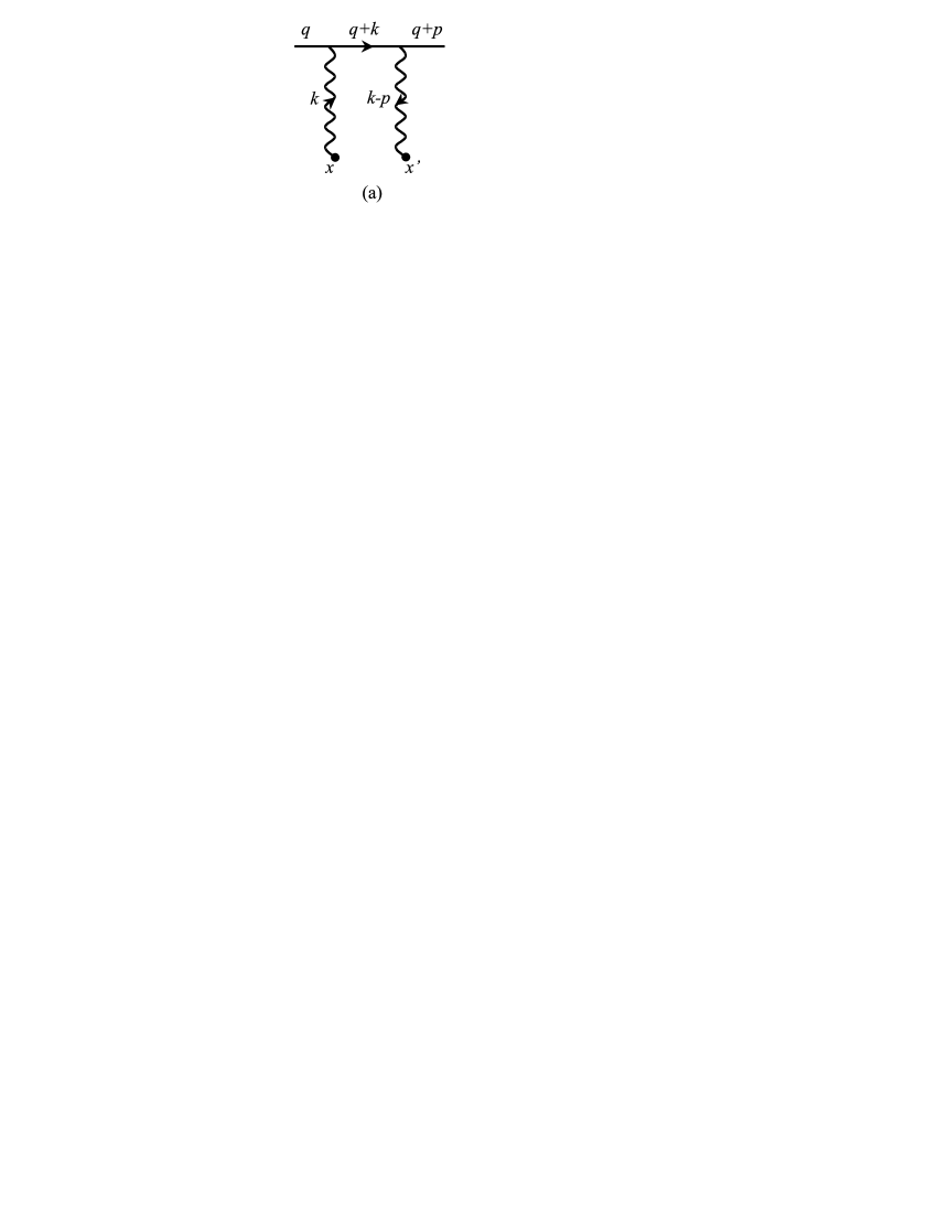
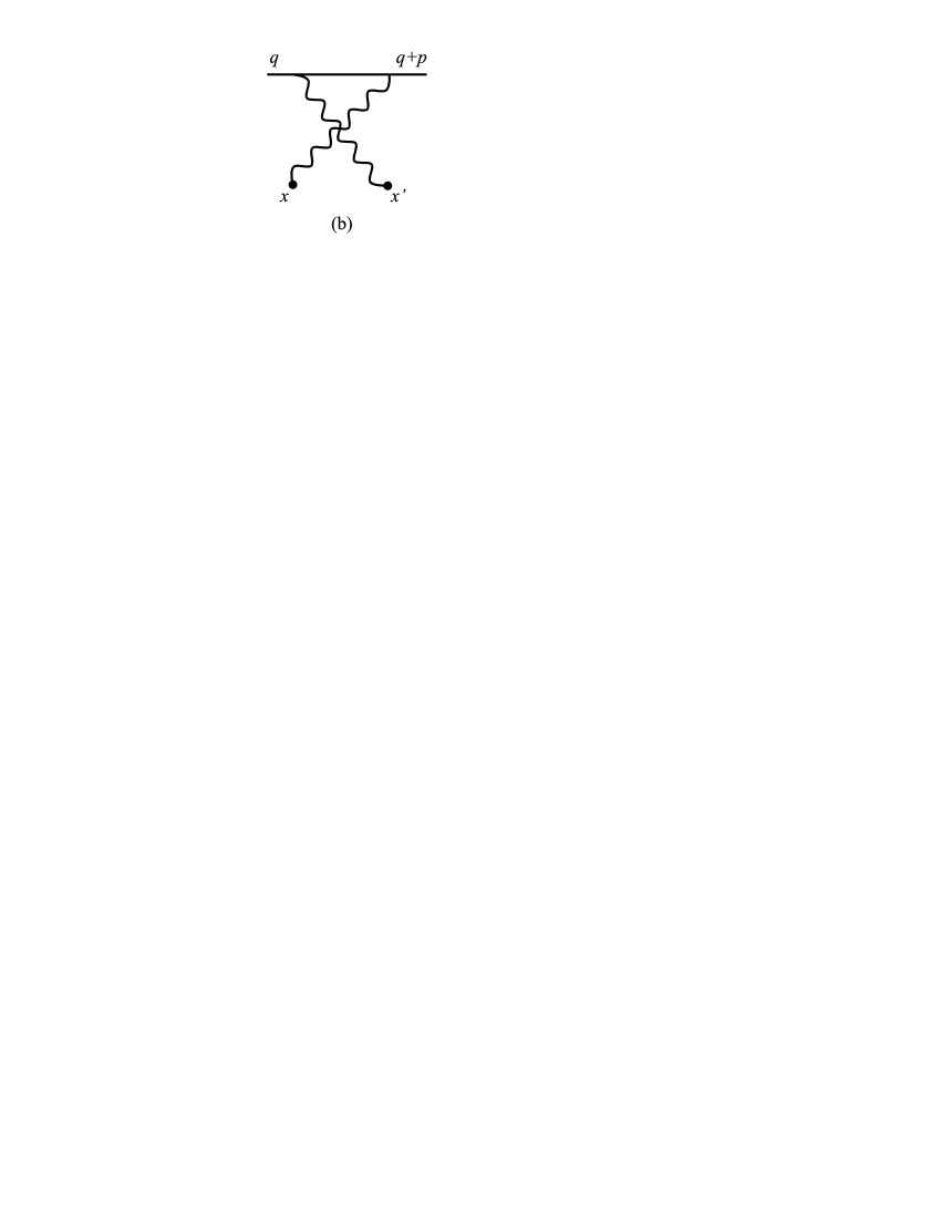
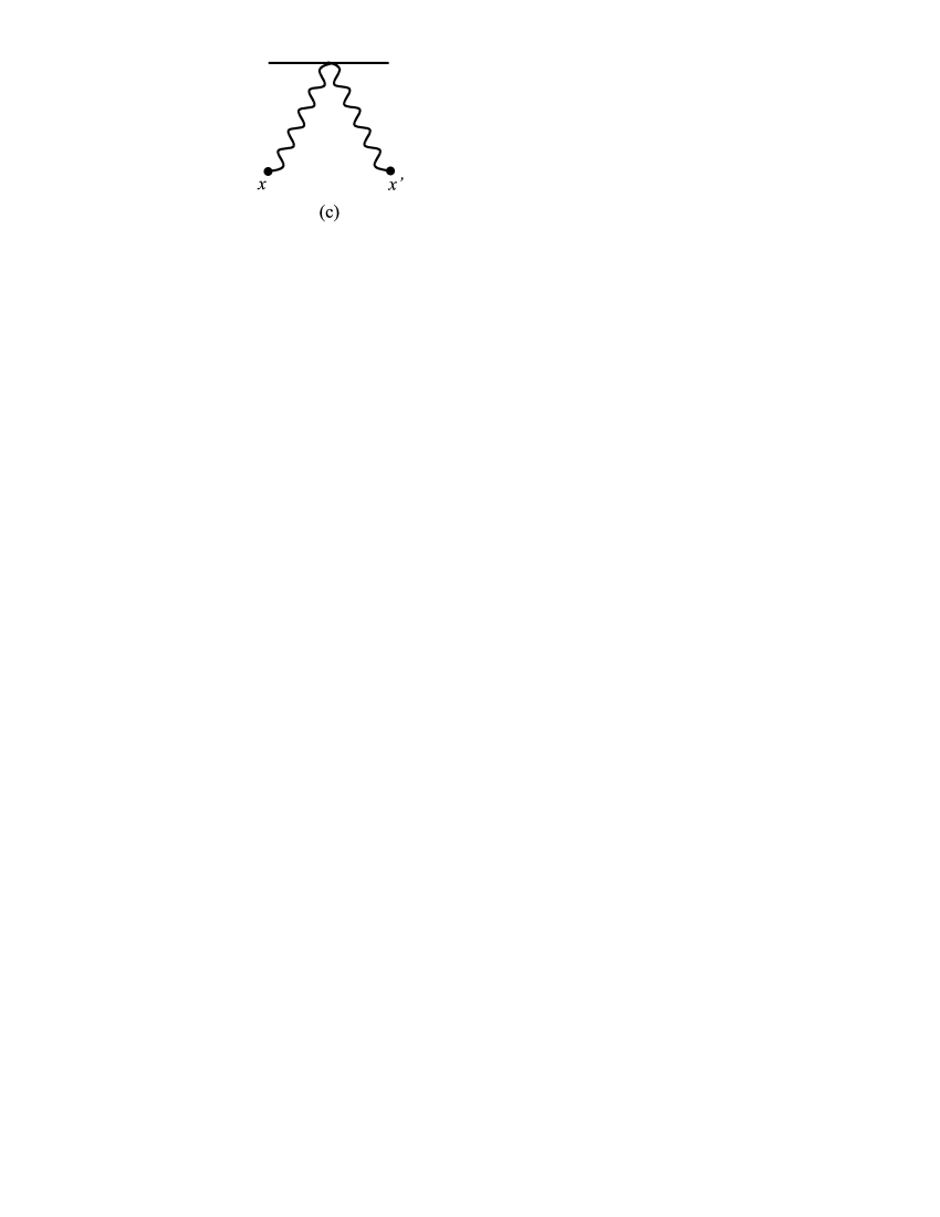
Figure 1: Kazakov, Quantum fluctuations of Coulomb potential as a source of flicker noise. The influence of heat bath

The tree contribution to the right hand side of Eq. (2) when the influence of external electric field is neglected is shown in Fig. 1. Repeating the argument of Ref. kazakov2 , it is not difficult to show that the leading contribution is contained in the diagrams 1(a), 1(b). Distinguishing their contributions by the corresponding Latin subscript, we have

$$G_{a}(x,x^{\prime}) = ie^{2}\iint d^{4}zd^{4}z^{\prime}\left\{\mathfrak{D}(x,z)\left[\phi_{0}(z)\stackrel{{\scriptstyle\leftrightarrow}}{{\partial_{0}}}\mathfrak{D}^{\phi}(z,z^{\prime})\stackrel{{\scriptstyle\leftrightarrow}}{{\partial_{0}^{\,\prime}}}\phi^{*}_{0}(z^{\prime})\right]\mathfrak{D}(z^{\prime},x^{\prime})\right\}_{11}\,,$$ (17)

$$G_{b}(x,x^{\prime}) = G_{a}(x^{\prime},x)\,,$$

where

$$\varphi\stackrel{{\scriptstyle\leftrightarrow}}{{\partial_{0}}}\psi = \varphi\partial_{0}\psi-\psi\partial_{0}\varphi\,,$$

and $\phi_{0}$ is the given particle state. Going over to momentum space with the help of Eqs. (5), (8), introducing the spectral function for $G_{a}(x,x^{\prime})$ according to Eq. (II.2), and writing the matrix product longhand yields

$$G_{a}(\bm{x},\bm{x}^{\prime},t^{\prime},\omega) = (4\pi e)^{2}\iint\frac{d^{3}\bm{q}}{(2\pi)^{3}}\frac{d^{3}\bm{p}}{(2\pi)^{3}}\frac{a(\bm{q})a^{*}(\bm{q}+\bm{p})}{\sqrt{2\varepsilon_{\bm{q}}2\varepsilon_{{\bm{q}}+\bm{p}}}}e^{ip^{0}(t^{\prime}-t_{0})-i\bm{p}\bm{x}^{\prime}}J_{a}(p,q,\bm{x}-\bm{x}^{\prime},\omega)\,,$$

$$p^{0} = \varepsilon_{\bm{q}+\bm{p}}-\varepsilon_{\bm{q}}\,,\quad\varepsilon_{\bm{q}}=+\sqrt{\bm{q}^{2}+m^{2}}\,,$$ (18)

where

$$J_{a}(p,q,\bm{x}-\bm{x}^{\prime},\omega)=-i\int\frac{d^{3}\bm{k}}{(2\pi)^{3}}e^{i\bm{k}(\bm{x}^{\prime}-\bm{x})}(2q_{0}+k_{0})(2q_{0}+k_{0}+p_{0})$$

$$\times\left[D_{11}(k)D^{\phi}_{11}(q+k)D_{11}(k-p)+D_{12}(k)D^{\phi}_{22}(q+k)D_{21}(k-p)\right]_{k_{0}=\omega}\,.$$ (19)

Here $q_{\mu}$ is the particle 4-momentum, $a(\bm{q})$ its momentum wave function at some time instant $t_{0},$ normalized by

$$\int\frac{d^{3}\bm{q}}{(2\pi)^{3}}|a(\bm{q})|^{2}=1\,,$$ (20)

and it is taken into account that $D^{\phi}_{12}=0\,.$

The second term in the square brackets in Eq. (III.1) can be neglected. Indeed, in view of the factor $D_{12}(k)$ which is proportional to $\delta(k^{2}),$ and the condition $k_{0}=\omega,$ the momentum $k$ contributes only a tiny value to the argument of the factor $D_{21};$ for electrons in a crystal, for instance, the ratio $|\bm{k}|/|\bm{p}|$ is of the order $(\hbar\omega/c)/(\hbar/d)=\omega d/c\approx\omega\cdot 10^{-18}\,{\rm s}.$ Therefore, this factor can be written simply as $D_{21}(p)\sim\delta(p^{2}).$ On the other hand, momentum transfer $p$ to the massive particle is spacelike, and hence the argument of the delta-function is always nonzero. Furthermore, using explicit expression for the photon propagator, the first term in the square brackets reads

$$\left\{\frac{1}{k^{2}+i0}-\frac{2\pi i\delta(k^{2})}{e^{\beta|k_{0}|}-1}\right\}D^{\phi}_{11}\left\{\frac{1}{(k-p)^{2}+i0}-\frac{2\pi i\delta((k-p)^{2})}{e^{\beta|k_{0}-p_{0}|}-1}\right\}=\frac{1}{[k^{2}+i0]}D^{\phi}_{11}\frac{1}{[(k-p)^{2}+i0]}$$

$$-\frac{2\pi i\delta(k^{2})}{e^{\beta|k_{0}|}-1}D^{\phi}_{11}\frac{1}{(k-p)^{2}+i0}-\frac{1}{k^{2}+i0}D^{\phi}_{11}\frac{2\pi i\delta((k-p)^{2})}{e^{\beta|k_{0}-p_{0}|}-1}+\frac{2\pi i\delta(k^{2})}{e^{\beta|k_{0}|}-1}D^{\phi}_{11}\frac{2\pi i\delta((k-p)^{2})}{e^{\beta|k_{0}-p_{0}|}-1}\,.$$

As before, the last term on the right hand side can be neglected, while the first term, describing the zero-temperature contribution, has already been considered in Ref. kazakov2 . Furthermore, $k_{0}$ enters the temperature exponent in the third term in the combination $(k_{0}-p_{0}),$ and, therefore, this term does not contribute to the leading order in $1/\omega,$ because in practice $|\omega|\ll p_{0}.$ Indeed, estimating the energy transfer as $p_{0}\approx(\bm{p}\bm{q})/m,$ and taking $|\bm{p}|\sim 1/l,$ where $l$ is the characteristic sample length, one finds for our standard example $|\omega/p_{0}|\sim 10^{-8}|\omega|l,$ where $l,\omega$ are supposed to be expressed in the $CGS$ system of units. Even for $l$ as large as $1\,{\rm cm},$ this ratio is very small for all practically relevant frequencies. Thus, the contribution of the second term only remains to be considered. In view of the factor $\delta(k^{2}),$ the pole of the function $D_{11}(q+k)$ in this term does not contribute. This is again a consequence of the requirement that the momentum transfer to a massive particle on-shell be spacelike: conditions $k^{2}=0,$ $q^{2}=m^{2},$ and $(q+k)^{2}=m^{2}$ cannot be satisfied altogether. Hence, the scalar particle propagator can be written simply as $D_{11}(q+k)=-1/(2qk),$ or, assuming that the particle is nonrelativistic, $|\bm{q}|\ll m,$ as

$$D^{\phi}_{11}(q+k)=-\frac{1}{2m\omega}\,.$$ (21)

Finally, neglecting $k$ in comparison with $p$ in the factor $1/[(k-p)^{2}+i0],$ using $p^{2}<0$ to omit $i0,$ and retaining only terms singular in $\omega,$ we find

$$J_{a}(p,q,\bm{x}-\bm{x}^{\prime},\omega) = \frac{2\pi(2m+p_{0})}{\omega\beta|\omega|p^{2}}\int\frac{d^{3}\bm{k}}{(2\pi)^{3}}e^{i\bm{k}(\bm{x}^{\prime}-\bm{x})}\delta(\omega^{2}-\bm{k}^{2})$$ (22)

$$= \frac{(2m+p_{0})}{2\pi\omega\beta p^{2}}+O(\omega)\,.$$

The reason why $p_{0}$ has been kept along with $m$ in the numerator will become clear soon. As to the contribution of the diagram 1(b), changing $\bm{k}\to\bm{k}+\bm{p}$ in Eq. (III.1), and then $\bm{q}\to\bm{q}-\bm{p},$ $\bm{p}\to-\bm{p}$ in Eq. (III.1) shows that

$$G_{b}(\bm{x},\bm{x}^{\prime},t^{\prime},\omega)=G^{*}_{a}(\bm{x},\bm{x}^{\prime},t^{\prime},-\omega)\,.$$

Thus, the total contribution to the function $G(\bm{x},\bm{x}^{\prime},t^{\prime},\omega)$ is

$$G(\bm{x},\bm{x}^{\prime},t^{\prime},\omega) = G_{a}(\bm{x},\bm{x}^{\prime},t^{\prime},\omega)+G^{*}_{a}(\bm{x},\bm{x}^{\prime},t^{\prime},-\omega)\,.$$ (23)

It is seen from this relation and Eq. (22) that only imaginary part of $G_{a}$ gives rise to a nonzero contribution to the total Green function $G,$ and this part corresponds to the term proportional to $p_{0}$ on the right hand side of Eq. (22). Thus,

$$G(\bm{x},\bm{x}^{\prime},t^{\prime},\omega) = -\frac{8\pi e^{2}}{m^{2}\beta\omega}\iint\frac{d^{3}\bm{q}}{(2\pi)^{3}}\frac{d^{3}\bm{p}}{(2\pi)^{3}}a(\bm{q})a^{*}(\bm{q}+\bm{p})\frac{(\bm{p}\bm{q})}{\bm{p}^{2}}e^{ip_{0}(t^{\prime}-t_{0})-i\bm{p}\bm{x}^{\prime}}\,,$$ (24)

where, in the denominator, the energies $\varepsilon_{\bm{q}},\varepsilon_{\bm{q}+\bm{p}}$ have been replaced by $m,$ and $p^{0}$ neglected in comparison with $|\bm{p}|$ on account of the condition $|\bm{q}|\ll m,$ while in the numerator, $p^{0}$ has been replaced by its leading long-range term, $(\bm{p}\bm{q})/m.$ It is instructive to see what the right hand side of Eq. (24) becomes in a particulary simple model case when the amplitude $a(\bm{q})$ can be written as

$$a(\bm{q})=b(\bm{q})e^{-i\bm{q}\bm{x}_{0}}\,,$$ (25)

where $b(\bm{q})$ is a real function of the particle momentum. In this case, $\bm{x}_{0}$ is easily identified as the mean particle position, and hence, the function $b(\bm{q})$ describes the momentum space profile of the particle wave packet. After extraction of the position-dependent phase factor, the amplitude becomes a relatively slowly varying function of the particle momentum, therefore, to the leading order of the long-range expansion, $b(\bm{q}+\bm{p})$ in the integrand of Eq. (24) can be replaced by $b(\bm{q})$

$$G(\bm{x},\bm{x}^{\prime},t^{\prime},\omega) = -\frac{8\pi e^{2}}{m^{2}\beta\omega}\iint\frac{d^{3}\bm{q}}{(2\pi)^{3}}\frac{d^{3}\bm{p}}{(2\pi)^{3}}|b(\bm{q})|^{2}\frac{(\bm{p}\bm{q})}{\bm{p}^{2}}e^{ip_{0}(t^{\prime}-t_{0})+i\bm{p}(\bm{x}^{\prime}-\bm{x}_{0})}\,,$$ (26)

In the exponent, $p_{0}$ generally cannot be replaced by $(\bm{p}\bm{q})/m,$ because the subleading term of its long-range expansion, $\bm{p}^{2}/(2m),$ although small compared to $(\bm{p}\bm{q})/m,$ can change the phase significantly, provided that the difference $(t^{\prime}-t_{0})$ is sufficiently large, as is the case if the particle collisions are neglected. However, taking into account the latter reduces this difference to the particle mean free time, $\tau_{f},$ so that the product $p_{0}(t^{\prime}-t_{0})$ can be completely neglected. Indeed, $\tau_{f}$ can be estimated roughly as $d/(|\bm{q}|/m),$ and hence, $p_{0}(t^{\prime}-t_{0})\sim|\bm{p}||\bm{q}|\tau_{f}/m\sim d|\bm{p}|\sim d/|\bm{x}^{\prime}-\bm{x}_{0}|\ll 1.$ Then the $\bm{p}$ integral can be evaluated with the help of the formula

$$\int\frac{d^{3}\bm{p}}{(2\pi)^{3}}e^{i(\bm{p}\bm{x})}\frac{4\pi\bm{p}}{\bm{p}^{2}}=\frac{i\bm{x}}{|\bm{x}|^{3}}\,,$$

yielding

$$G(\bm{x},\bm{x}^{\prime},t^{\prime},\omega) = -2i\frac{e^{2}}{m^{2}\beta\omega}\frac{(\overline{\bm{q}}\bm{r}^{\prime})}{r^{\prime 3}}\,,\quad\bm{r}^{\prime}=\bm{x}^{\prime}-\bm{x}_{0}\,,$$ (27)

where the overline denotes $\bm{q}$-averaging over the given particle state. In the absence of external electric field, $\overline{\bm{q}}$ is zero, and therefore so is the right hand side of Eq. (27). As we will see in the next section, the same result is obtained in the general case without the use of the model decomposition (25). But even for nonzero $\overline{\bm{q}},$ the voltage power spectrum calculated from $G$ given by Eq. (27) turns out to be zero. This is verified directly by substituting expression (27) into Eqs. (16), (14). The reason for nullification of the voltage power spectrum is easily identified – it is the consequence of the fact that the function $G_{a}(\bm{x},\bm{x}^{\prime},t^{\prime},\omega)$ is independent of the $\bm{x}$ coordinate. The $\bm{x}$-dependence has been lost upon extracting the low-frequency asymptotic of $J_{a}$ in Eq. (22).

III.2 The influence of external electric field and particle collisions

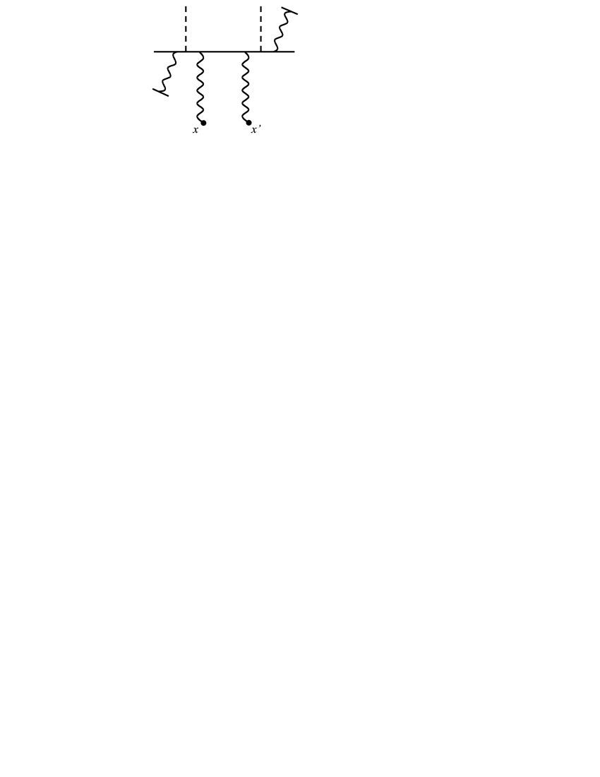
Figure 2: Kazakov, Quantum fluctuations of Coulomb potential as a source of flicker noise. The influence of heat bath

Let us now consider corrections to the power spectrum due to constant homogeneous external electric field, taking into account also the influence of particle collisions. These corrections are twofold. First of all, the field affects the particle wave function $a(\bm{q}),$ which is symbolized in Fig. 2 by inserting the vertices of particle-field interaction into the two external solid lines. This is only a schematic picture, because the effect of a constant homogeneous field on the free particle states cannot be treated perturbatively. The latter circumstance, however, is not important in view of the particle collisions which prevent the particle from gaining too much momentum from the field, thus cutting down its effect (particle collisions are symbolized in Fig. 2 by a virtual photon interchange between particles). Account of these two factors is accomplished by replacing the particle momentum probability distribution, $|a(\bm{q})|^{2},$ by the statistical distribution function, obtained as a solution of the kinetic equation in the presence of external electric field. This point will be discussed in more detail later in this section.

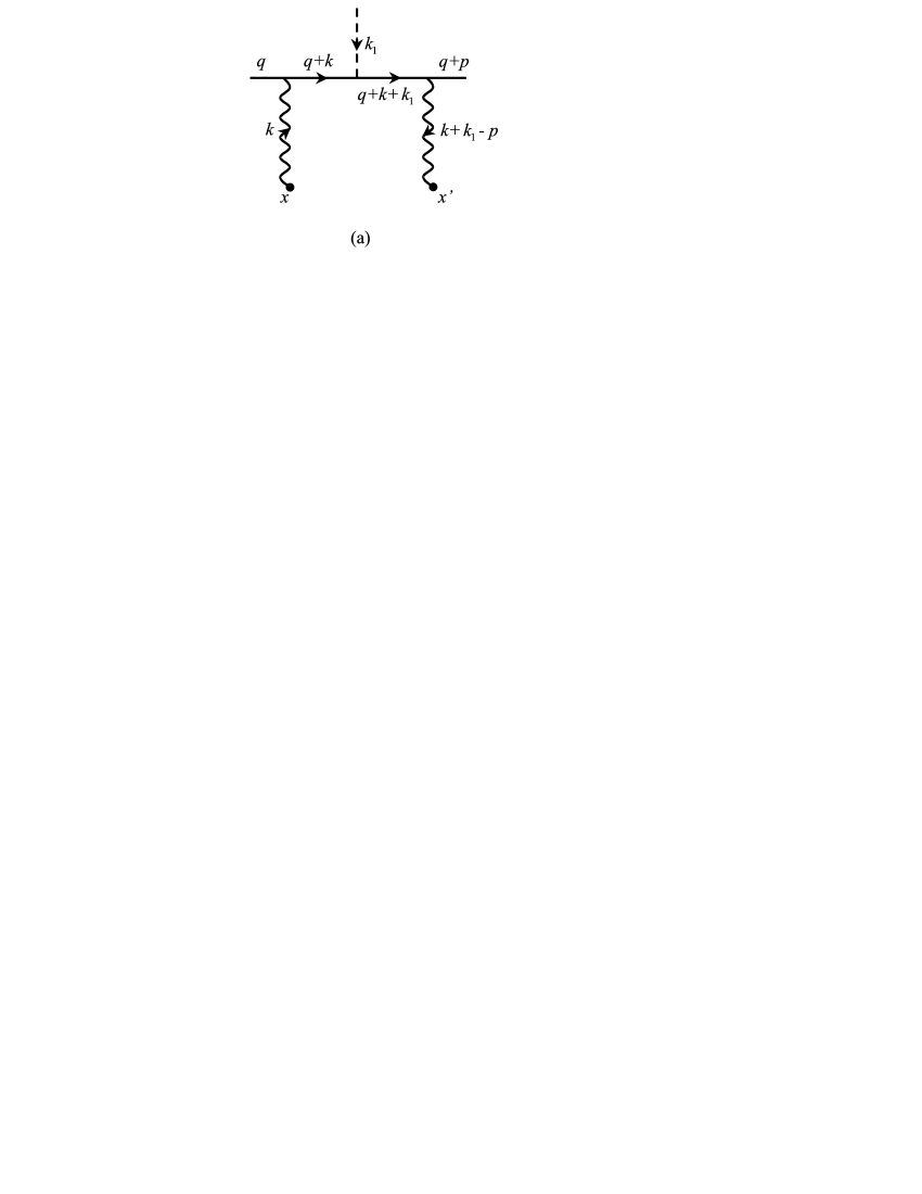
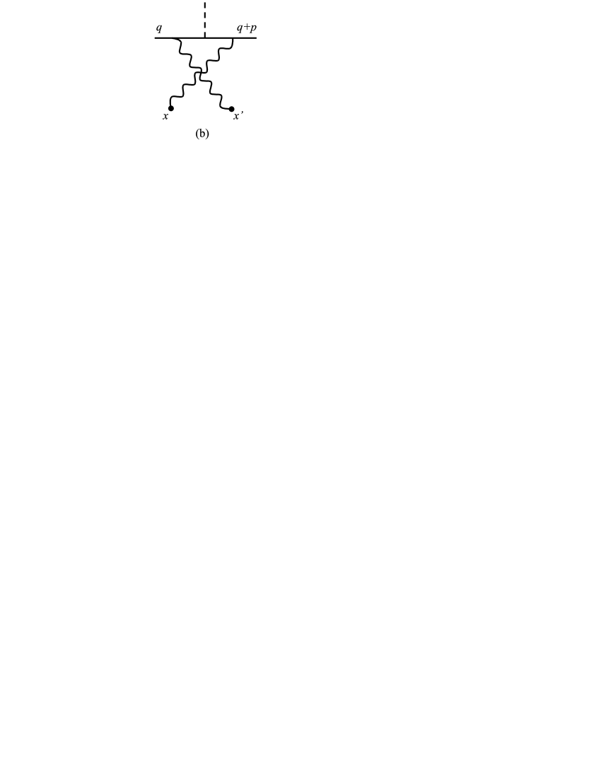
Figure 3: Kazakov, Quantum fluctuations of Coulomb potential as a source of flicker noise. The influence of heat bath

Next, the particle propagator is also modified by the external field. It is not difficult to see that for a sufficiently small field strength, $\bm{E},$ this modification can be treated perturbatively. It can be recalled that in coordinate space, it amounts to multiplying the zero-field propagator $D^{\phi}(z,z^{\prime})$ by $\exp\left\{ie(\bm{E},\bm{z}+\bm{z}^{\prime})(z^{\prime}_{0}-z_{0})/2\right\}.$ Although the low-frequency limit is determined by the large-time behavior of the quantities involved, implying that $(z^{\prime}_{0}-z_{0})\sim 1/\omega$ is large, the exponent can be made as small as desired for any given $\omega$ by taking $|\bm{E}|$ sufficiently small. This also will be clear from the explicit calculations to follow. The lowest order correction to the correlation function is represented by diagrams with a single insertion of the particle-field interaction vertex into the internal solid line, as shown in Fig. 3. As in the preceding section, these diagrams vanish unless all interaction vertices are 1-type, on account of momentum conservation in the vertices together with the mass shell conditions for the massive particle. The contribution of the diagram 3(a) to the spectral density of the two-point Green function

$$G^{E}_{a}(\bm{x},\bm{x}^{\prime},t^{\prime},\omega)= (4\pi e)^{2}\iiint\frac{d^{3}\bm{q}}{(2\pi)^{3}}\frac{d^{3}\bm{p}}{(2\pi)^{3}}\frac{d^{3}\bm{k}_{1}}{(2\pi)^{3}}\frac{a(\bm{q})a^{*}(\bm{q}+\bm{p})}{\sqrt{2\varepsilon_{\bm{q}}2\varepsilon_{{\bm{q}}+\bm{p}}}}$$ (28)

$$\times e^{ip^{0}(t^{\prime}-t_{0})-i(\bm{p}-\bm{k}_{1})\bm{x}^{\prime}}\varphi(\bm{k}_{1})J^{E}_{a}(p,q,\bm{x}-\bm{x}^{\prime},\omega)\,,$$

where

$$J^{E}_{a}(p,q,\bm{x}-\bm{x}^{\prime},\omega)=-\left.ie\int\frac{d^{3}\bm{k}}{(2\pi)^{3}}e^{i\bm{k}(\bm{x}^{\prime}-\bm{x})}(2q_{0}+k_{0})(2q_{0}+2k_{0})(2q_{0}+k_{0}+p_{0})\right.$$

$$\left.D_{11}(k)D^{\phi}_{11}(q+k)D^{\phi}_{11}(q+k+k_{1})D_{11}(k+k_{1}-p)\right|_{k_{0}=\omega}\,,\quad k_{1}=(0,\bm{k}_{1})\,,$$ (29)

and $\varphi(\bm{k})$ is the Fourier transform of the external field potential, $\varphi(\bm{x})=-(\bm{E},\bm{x}).$ We do not include an arbitrary constant in this expression because it is clear in advance that it cannot affect the final result. It is proved in the Appendix that the correlation function is actually invariant under the most general gauge variations of the electromagnetic potential. Substituting

$$\varphi(\bm{k})=-i(2\pi)^{3}\left(\bm{E}\frac{\partial}{\partial\bm{k}}\right)\delta^{(3)}(\bm{k})$$

into Eq. (28) and integrating by parts, the $\bm{k}_{1}$ integral in Eq. (28) is brought to the form

$$i\int d^{3}\bm{k}_{1}\delta^{(3)}(\bm{k})\left(\bm{E}\frac{\partial}{\partial\bm{k}_{1}}\right)\left[D^{\phi}_{11}(q+k+k_{1})D_{11}(k+k_{1}-p)e^{-i(\bm{p}-\bm{k}_{1})\bm{x}^{\prime}}\right]\,,$$ (30)

where only terms involving $\bm{k}_{1}$ are retained. As we have seen, the singularity at $\omega=0$ in the function $G_{a}(\bm{x},\bm{x}^{\prime},t^{\prime},\omega)$ comes from integration over small $\bm{k},$ and this singularity is now strengthened by the extra particle propagator and the differentiation with respect to $\bm{k}_{1}.$ Consider first the case when the $\bm{k}_{1}$-derivative acts on the last two factors in the square brackets. Since these depend on the difference $(\bm{p}-\bm{k}_{1}),$ changing $\partial/\partial\bm{k}_{1}\to-\partial/\partial\bm{p},$ and then integrating by parts with respect to $\bm{p}$ in Eq. (28), this derivative is rendered to act on terms independent of $\bm{k}$. Thus, of the three factors in the square brackets, only the first is to be differentiated in effect, thus reducing the expression (30) to

$$\frac{2i(\bm{E},\bm{q}+\bm{k})}{[m^{2}-(q+k)]^{2}}D_{11}(k-p)e^{-i(\bm{p}\bm{x}^{\prime})}\,.$$

Taking into account also the vertex factor $e(2q_{0}+2k_{0}),$ we see that the first order correction to the charged particle propagator due to constant homogeneous external electric field is obtained by inserting the factor

$$\frac{4ie(q_{0}+k_{0})(\bm{E},\bm{q}+\bm{k})}{[m^{2}-(q+k)]^{2}}\equiv\varkappa$$

into the integrand in Eq. (III.1). The rest of the calculation repeats the steps of Sec. III.1. Substituting explicit expressions for the photon propagators, one sees that only the part proportional to $\delta(k^{2})$ is to be retained in the expression for $D_{11}(k),$ while the corresponding part in $D_{11}(k-p)$ is to be omitted. One consequence of this observation is that the factor $\varkappa$ simplifies to

$$\frac{ie(\bm{E}\bm{q})}{m\omega^{2}}\,,$$

where we have taken into account that $k_{0}=\omega\ll q_{0},$ and $|\bm{k}|=|\omega|\ll|\bm{q}|$ [indeed, taking our standard example of electron in a crystal, the ratio $|\omega|/|\bm{q}|$ is, in the ordinary units, $(\hbar|\omega|/c)/|\bm{q}|\sim|\omega|d/c\sim|\omega|10^{-18},$ with $\omega$ expressed in Hz]. Another consequence is that the contributions of diagrams 3(a), 3(b) are related, as before, by

$$G^{E}_{b}(\bm{x},\bm{x}^{\prime},t^{\prime},\omega)=G^{E*}_{a}(\bm{x},\bm{x}^{\prime},t^{\prime},-\omega)\,.$$

Furthermore, Eq. (22) is now replaced by

$$J^{E}_{a}(p,q,\bm{x}-\bm{x}^{\prime},\omega) = \varkappa\frac{2\pi(2m+p_{0})}{\omega\beta|\omega|p^{2}}\int\frac{d^{3}\bm{k}}{(2\pi)^{3}}e^{i\bm{k}(\bm{x}^{\prime}-\bm{x})}\delta(\omega^{2}-\bm{k}^{2})$$ (31)

$$= \frac{ie(\bm{E}\bm{q})}{m\omega^{2}}\frac{(2m+p_{0})}{2\pi\omega\beta p^{2}}\left[1-\frac{\omega^{2}}{6}(\bm{x}^{\prime}-\bm{x})^{2}\right]+O(\omega)\,.$$

An important difference in comparison with the result of the preceding section is that because of the extra imaginary unit brought in by the factor $\varkappa,$ the term proportional to $p_{0}$ in the last formula gives rise now to a purely real contribution upon substituting $J^{E}_{a}$ in Eq. (28), and hence is cancelled in the sum of diagrams 3(a), 3(b). On the other hand, the terms independent of $p_{0}$ survive, and lead to the following expression for the first order correction to the spectral density of the two-point Green function

$$G^{E}(\bm{x},\bm{x}^{\prime},t^{\prime},\omega)=-\frac{16\pi ie^{3}}{m\beta\omega^{3}} \left[1-\frac{\omega^{2}}{6}(\bm{x}^{\prime}-\bm{x})^{2}\right]$$ (32)

$$\times{\rm Re}\iint\frac{d^{3}\bm{q}}{(2\pi)^{3}}\frac{d^{3}\bm{p}}{(2\pi)^{3}}a(\bm{q})a^{*}(\bm{q}+\bm{p})\frac{(\bm{E}\bm{q})}{\bm{p}^{2}}e^{ip_{0}(t^{\prime}-t_{0})-i(\bm{p}\bm{x}^{\prime})}\,.$$

In a many-particle system, this result is to be expressed through the one-particle density matrix, which is accomplished by replacing $a^{*}(\bm{q}^{\prime})a(\bm{q})\to\varrho_{0}(\bm{q}^{\prime},\bm{q}),$ where $\varrho_{0}$ is the momentum space density matrix at the time instant $t_{0}.$ We recall that $t_{0}$ denotes the instant at which the particle state $a(\bm{q})$ is prepared. It can be identified, for instance, as the moment the charge carrier enters the sample, or escapes from a surface trap, etc. The factor $e^{ip_{0}(t^{\prime}-t_{0})}$ in the integrand then realizes time evolution of the density matrix from $t_{0}$ to $t^{\prime}.$ Since $p_{0}=(\bm{q}+\bm{p})^{2}/2m-\bm{q}^{2}/2m,$ this is a free evolution. The fact that the evolution of charge carriers in solids is not actually free on macroscopic scales is not important for the present consideration in which appearance of the $1/\omega$-singularity is related to the effects of the medium on the field propagators. In this respect, it is essentially different from considerations of Ref. kazakov2 , in which time evolution of the particle wave packet was the central issue, and, in particular, the requirement that the particle collisions be elastic was important. To take into account particle collisions in the present case, it is sufficient to consider them as instantaneous. Then the interval $(t_{0},t^{\prime})$ is divided into a sequence of short time intervals of order $\tau_{f}$ (the particle mean free time), on each of which the density matrix evolves freely as in Eq. (32), and changes abruptly at the collision instants. Going through this sequence the density matrix tends to the stationary statistical distribution function, $\varrho(\bm{q}^{\prime},\bm{q}),$ which is independent of the initial particle state. What is important here is the sign of the difference $(t^{\prime}-t_{0}).$ Recall that $t^{\prime}$ is a fixed time instant to count off the time interval $\tau$ with respect to which the correlation function is Fourier-transformed, and that each particle has its own $t_{0}.$ This means that for a given $\omega,$ the system is observed during the time interval $(t^{\prime}-\Delta t,t^{\prime}+\Delta t),$ where $\Delta t\sim 1/\omega,$ and $t_{0}$s are distributed uniformly over this interval. The density matrix evolves forward (backward) in time, if $t^{\prime}>t_{0}$ ($t^{\prime}<t_{0}$). But time reversal involves inversion of particle momentum, and therefore, the reciprocal contributions to the function $G^{E}(\bm{x},\bm{x}^{\prime},t^{\prime},\omega)$ have opposite signs. To be more specific, let $(t^{\prime}-t_{0})>0.$ Then the exponent $e^{ip_{0}(t^{\prime}-t_{0})}$ realizes a forward evolution of the density matrix, so that the integral in Eq. (32) takes eventually the form

$$\iint\frac{d^{3}\bm{q}}{(2\pi)^{3}}\frac{d^{3}\bm{p}}{(2\pi)^{3}}\varrho(\bm{q}+\bm{p},\bm{q})\frac{(\bm{E}\bm{q})}{\bm{p}^{2}}e^{-i(\bm{p}\bm{x}^{\prime})}\,.$$ (33)

On the other hand, if $(t^{\prime}-t_{0})<0,$ then the density matrix evolves backward. In momentum space, the initial state of the reversed motion is represented by the amplitude $\tilde{a}(\bm{q})=a^{*}(-\bm{q}).$ Taking complex conjugate of the integral in Eq. (32) (which does not change the value of $G^{E}$ in view of the sign “Re”), and changing the integration variables $\bm{q}\to-\bm{q},$ $\bm{p}\to-\bm{p}$ gives in this case

$$-\iint\frac{d^{3}\bm{q}}{(2\pi)^{3}}\frac{d^{3}\bm{p}}{(2\pi)^{3}}\tilde{a}(\bm{q})\tilde{a}^{*}(\bm{q}+\bm{p})\frac{(\bm{E}\bm{q})}{\bm{p}^{2}}e^{ip_{0}(t_{0}-t^{\prime})-i(\bm{p}\bm{x}^{\prime})}\,.$$

After replacement $\tilde{a}^{*}(\bm{q}+\bm{p})\tilde{a}(\bm{q})\to\tilde{\varrho}(\bm{q}+\bm{p},\bm{q}),$ where $\tilde{\varrho}$ plays the role of the momentum density matrix at the moment $t^{\prime},$ the exponent $e^{ip_{0}(t_{0}-t^{\prime})}$ governs forward evolution of this state on the interval $(t^{\prime},t_{0}),$ so that the above expression takes the form

$$-\iint\frac{d^{3}\bm{q}}{(2\pi)^{3}}\frac{d^{3}\bm{p}}{(2\pi)^{3}}\varrho(\bm{q}+\bm{p},\bm{q})\frac{(\bm{E}\bm{q})}{\bm{p}^{2}}e^{-i(\bm{p}\bm{x}^{\prime})}\,.$$

The density matrix here is the same as in (33), because the statistical distribution is independent of the initial state. We see that reciprocal contributions to the function $G^{E}(\bm{x},\bm{x}^{\prime},t^{\prime},\omega)$ cancel each other when summed over all particles in the system. Thus, we arrive at the important conclusion that the total noise intensity is independent of the number of particles, and remains at the level of individual contribution. As was shown in Ref. kazakov2 , this conclusion is also true of the disconnected part of the correlation function, though by virtue of quite different reasons.

It is customary to further express the function $\varrho(\bm{q}^{\prime},\bm{q})$ via the real mixed distribution function, $n(\bm{r},\bm{q}),$ according to

$$\varrho(\bm{q}+\bm{p},\bm{q})=\int d^{3}\bm{r}e^{i(\bm{p}\bm{r})}n\left(\bm{r},\bm{q}+\frac{\bm{p}}{2}\right)\,.$$

Probability distributions for the particle position in a sample and for its momentum can be obtained by integrating $n(\bm{r},\bm{p})$ over all $\bm{p}$ and the sample volume, respectively. Using this in the expression (33), and substituting the latter into Eq. (32) yields

$$G^{E}(\bm{x},\bm{x}^{\prime},t^{\prime},\omega)=-\frac{16\pi ie^{3}}{m\beta\omega^{3}} \left[1-\frac{\omega^{2}}{6}(\bm{x}^{\prime}-\bm{x})^{2}\right]$$ (34)

$$\times{\rm Re}\iiint\frac{d^{3}\bm{q}}{(2\pi)^{3}}\frac{d^{3}\bm{p}}{(2\pi)^{3}}d^{3}\bm{r}\frac{(\bm{E}\bm{q})}{\bm{p}^{2}}n\left(\bm{r},\bm{q}+\frac{\bm{p}}{2}\right)e^{i\bm{p}(\bm{r}-\bm{x}^{\prime})}\,.$$

As we know, the first term in the square brackets in this formula doest not contribute to the voltage power spectrum, and can be omitted. Furthermore, after shifting $\bm{q}\to\bm{q}-\bm{p}/2,$ and omitting the imaginary term proportional to $(\bm{E},\bm{p}),$ the triple integral becomes purely real, so the symbol “${\rm Re}$” can be omitted. Integrating then over $\bm{p}$ with the help of the formula

$$\int\frac{d^{3}\bm{p}}{(2\pi)^{3}}e^{i(\bm{p}\bm{x})}\frac{4\pi}{\bm{p}^{2}}=\frac{1}{|\bm{x}|}\,,$$

we thus obtain

$$G^{E}(\bm{x},\bm{x}^{\prime},t^{\prime},\omega)=\frac{2ie^{3}(\bm{x}^{\prime}-\bm{x})^{2}}{3m\beta\omega}\iint\frac{d^{3}\bm{q}}{(2\pi)^{3}}d^{3}\bm{r}(\bm{E}\bm{q})\frac{n(\bm{r},\bm{q})}{|\bm{r}-\bm{x}^{\prime}|}\,.$$ (35)

Equation (16) shows that the spectral density of the correlation function is given by the same expression (35), so that the power spectrum of voltage fluctuations is, according to Eq. (14),

$$C_{U}(\bm{x},\bm{x}^{\prime},t^{\prime},\omega)=-\frac{2ie^{3}(\bm{x}^{\prime}-\bm{x})^{2}}{3\beta\omega\Omega}\int d^{3}\bm{r}(\bm{E}\overline{\bm{v}}(\bm{r}))\left(\frac{1}{|\bm{r}-\bm{x}|}+\frac{1}{|\bm{r}-\bm{x}^{\prime}|}\right)\,,$$ (36)

where

$$\overline{\bm{v}}(\bm{r})=\Omega\int\frac{d^{3}\bm{q}}{(2\pi)^{3}}\frac{\bm{q}}{m}n(\bm{r},\bm{q})$$

is the local drift velocity of the charge carriers, $\Omega$ denoting the sample volume. For a crystal in the homogeneous external field, $\overline{\bm{v}}$ is a function of the crystalline direction,

$$\overline{v}_{i}=\mu_{ik}E_{k}\,,\quad i,k=1,2,3,$$

where $\mu_{ik}$ is the charge carrier mobility tensor. With the help of this formula Eq. (36) can be rewritten as

$$C_{U}(\bm{x},\bm{x}^{\prime},t^{\prime},\omega)=-i\eta\,\frac{U^{2}_{0}}{\omega}\,,\quad\eta\equiv\frac{2e^{3}\mu g}{3\beta}\,,$$ (37)

where

$$\mu=\mu_{ik}n_{i}n_{k}\,,\quad\bm{n}=\frac{\bm{E}}{|\bm{E}|}\,,$$

$U_{0}=|\bm{E}||\bm{x}-\bm{x}^{\prime}|$ is the bias applied to the sample (it is assumed that $\bm{E}\parallel(\bm{x}-\bm{x}^{\prime}),$ as is usually the case), and $g$ is a geometrical factor

$$g\equiv\frac{1}{\Omega}\int\limits_{\Omega}d^{3}\bm{r}\left(\frac{1}{|\bm{r}-\bm{x}|}+\frac{1}{|\bm{r}-\bm{x}^{\prime}|}\right)\,.$$ (38)

If Fourier transformation is defined in a purely real form, i.e., as a decomposition in $\cos(\omega\tau),$ $\sin(\omega\tau),$ rather than in $e^{i\omega\tau},$ then the spectral density is also real:

$$C_{U}(\bm{x},\bm{x}^{\prime},t^{\prime},\omega)=\eta\,\frac{U^{2}_{0}}{\omega}\,,\quad\eta\equiv\frac{2e^{3}\mu g}{3\beta}\,,$$ (39)

We mention for future reference that if the sample is an elongated parallelepiped with the leads attached to its ends (as is usually the case in practice), then the $g$-factor can be evaluated as

$$g\approx\frac{2}{lwh}\int\limits_{w}^{l}\frac{whdx}{x}=\frac{2}{l}\ln\frac{l}{w}\,,$$ (40)

where $l,w,h$ denote the sample length, width and thickness, respectively, and it is assumed that $h<w\ll l.$ We note also that in the ordinary units, the dimensionless factor $\eta$ reads

$$\eta=\frac{2e^{3}\mu g}{3\beta\hbar^{2}c^{3}}=\frac{2\alpha^{2}}{3ec}g\mu T\,,$$

$\alpha$ being the fine structure constant. In particular, in the $CGS$ system of units,

$$\eta\approx 3.4\cdot 10^{-22}g\mu T\,,$$ (41)

where the absolute temperature $T$ is to be expressed in ${}^{\circ}{\rm K}.$

III.3 On the unboundedness of $1/f$-spectrum

In this section, a special feature of the derived expression for the power spectrum, namely, its oddness in frequency, will be discussed in connection with the problem of observed absence of frequency limits of the $1/f$-law. As was mentioned in Introduction, $1/f$ noise has been detected in a very wide frequency band $\sim 10^{-6}\,{\rm Hz}$ to $10^{6}\,{\rm Hz}.$ This fact represents one of the essential difficulties for theoretical explanation, because all physical mechanisms underlying existing models of flicker noise work in much narrower subbands, and none of the models suggested so far has been able to explain the observed plenum of the $1/f$-spectrum.

On the other hand, existence of bounds on this spectrum is generally believed to be necessary in order to guarantee finiteness of the total noise power. There is a well-known argument flinn according to which these limits are actually unnecessary when the flicker noise exponent $\gamma$ is strictly equal to unity, because the logarithmic divergence of the total power is not a problem in this case in view of the existence of natural frequency cutoffs such as the inverse Planck time and lifetime of Universe. However, this reasoning does not work for $\gamma\neq 1,$ in which case divergence is a power of the cutoff. At the same time, the results obtained above reconcile unboundedness of $1/f$-spectrum with the requirements of stationarity and finiteness of the total noise power in a quite natural way. Indeed, using Eq. (37) we find

$$\int\limits_{-\infty}^{+\infty}\frac{d\omega}{2\pi}C_{U}(\bm{x},\bm{x}^{\prime},t^{\prime},\omega)e^{i\omega\tau}=\eta U^{2}_{0}\int\limits_{-\infty}^{+\infty}\frac{d\omega}{2\pi}\frac{\sin(\omega\tau)}{\omega}=\frac{\tau}{|\tau|}\frac{\eta U^{2}_{0}}{2}\,.$$

More generally, if the spectrum $C_{U}\sim 1/f^{\gamma}$ is continued to negative $f$’s as an odd function, then for any $0<\gamma<2$ the integral

$$\int\limits_{-\infty}^{+\infty}d\omega C_{U}e^{i\omega\tau}\sim\int\limits_{0}^{+\infty}df\frac{\sin(2\pi f\tau)}{f^{\gamma}}$$

is convergent in both limits $f\to 0$ and $f\to\infty.$ In particular, the singular contribution to the voltage variance (i.e. to the quantity $C_{U}(t,t^{\prime})|_{\tau=0}$) vanishes.

Since appearance of odd contributions to the power spectrum is somewhat unusual in macroscopic fluctuation theory, let us discuss it in more detail. Under stationary external conditions, the voltage noise power spectrum (to be denoted below simply as $C_{U}(t,t^{\prime}),$ with the spatial arguments suppressed, for brevity) must be independent of $t^{\prime}.$ This is an expression of the noise stationarity, or, using a term more suitable for the subsequent discussion, time homogeneity with respect to the macroscopic system. It is usually realized as the requirement that $C_{U}(t,t^{\prime})$ be a function of the difference $t-t^{\prime}\equiv\tau.$ Since $C_{U}(t,t^{\prime})$ is also symmetric with respect to the interchange $t\leftrightarrow t^{\prime},$ an immediate consequence of this is that it is actually a function of $|\tau|,$ and hence the spectral density is a real even function of frequency. It is important, on the other hand, that time homogeneity is not necessarily exhibited by individual contributions to the total voltage fluctuation, whatever mechanism of flicker noise generation be. In particular, this property evidently does not take place at the microscopic level, i.e., with respect to elementary processes such as charge carrier trapping, surface or grain boundary scattering, etc. Stationarity of the macroscopic process emerges usually upon summation over a large number of individual contributions, so that this microscopic inhomogeneity turns out to be inconsequential. However, this summation is not the only way to obtain a stationary correlation function symmetric in $t,t^{\prime}.$ Another possibility, which is realized in the present paper, is that flicker noise may be a one-particle phenomenon, in the sense that the entire effect can be ascribed to elementary fluctuations produced by single charge carriers. In this case the function $C_{U}(t,t^{\prime})$ does not have to depend solely on $|\tau|,$ and as the explicit calculations of Sec. III show, it actually does not. As was mentioned above, elementary processes are inhomogeneous in time, and hence the symmetry with respect to $t\leftrightarrow t^{\prime}$ imposes no restriction on the $\tau$-dependence of the correlation function. The only remaining requirement, namely reality of the correlation function, implies that contributions to the spectral density must be real even, or imaginary odd functions of frequency [Cf. Eq. (16)]. These two cases correspond to the Fourier decomposition of the function $C_{U}(t^{\prime}+\tau,t^{\prime})$ in $\cos(\omega\tau)$ and $\sin(\omega\tau),$ respectively, and describe the parts symmetric and antisymmetric with respect to the difference of its time arguments. Finally, transition to the statistical distribution removes the $t^{\prime}$-dependence of the power spectrum [Cf. transition from Eq. (32) to Eq. (34)]. This restores macroscopic time homogeneity of the correlation function, but leaves the possibility of being odd with respect to the difference of its time arguments. In other words, dependence of the power spectrum on $t^{\prime}$ shows itself only at microscopic scales, while macroscopically fluctuations look as if they were homogeneous in time.

The $1/f$-spectrum derived in the previous section has no lower frequency cutoff. As to the upper bound, it is given by the condition $f\ll T$ [see Sec. II.1], or in the ordinary units, $f\ll kT/\hbar\approx 10^{11}T\,{\rm Hz},$ with $T$ expressed in ${}^{\circ}{\rm K}.$ We see that from the practical point of view, the obtained spectrum has no upper cutoff either.

III.4 Validity of Eq. (39) and comparison with experimental data

Let us next discuss the range of applicability of the obtained results. The validity of the perturbative treatment of the external field imposes a very strong bound on the field strength. For this purpose we first collect all characteristic factors that have appeared in the course of extracting the $1/\omega$-asymptotic of the voltage power spectrum. As we have seen, insertion of the vertex describing interaction of the virtual charged particle with external field amounts to multiplying the zero-field diagram by the factor, in the ordinary units, $e(\bm{E}\bm{q})/(m\omega^{2}\hbar)\,,$ which is eventually promoted by the $\bm{q}$-integration into $e\mu\bm{E}^{2}/(\omega^{2}\hbar).$ Furthermore, the leading non-vanishing contribution to the voltage correlation function has been obtained after expanding $e^{i\bm{k}(\bm{x}-\bm{x}^{\prime})}$ in the integrand of the $\bm{k}$-integral, which brought in a factor $\omega^{2}(\bm{x}-\bm{x}^{\prime})^{2}/c^{2}.$ Thus, the overall factor is $e\mu\bm{E}^{2}(\bm{x}-\bm{x}^{\prime})^{2}/(c^{2}\hbar)=e\mu U^{2}_{0}/(c^{2}\hbar).$ This is small provided $\mu U^{2}_{0}\ll c^{2}\hbar/e\approx 10^{3}$ units $CGS,$ which is a quite soft requirement met in virtually all flicker noise measurements (Cf. examples below). The problem with this estimation, however, is that at higher orders, the scalar product $(\bm{E}\bm{q})$ is to be estimated as $|\bm{E}||\bm{q}|,$ because $\overline{(\bm{E}\bm{q})^{2}}$ is of the order $(|\bm{E}||\bm{q}|)^{2}\,,$ rather than $(\bm{E}\overline{\bm{q}})^{2}\,.$ As a result, the requirement that the factor $e(\bm{E}\bm{q})/(m\omega^{2}\hbar)$ be small leads to the following upper bound on the electric field strength for a given frequency $\omega,$ in the $CGS$ system of units, $|\bm{E}|\ll dm\omega^{2}/e\approx 10^{-25}\omega^{2}.$ At the same time, the values $|\bm{E}|\sim 1$ are quite normal in flicker noise measurements. In other words, from the point of view of the developed theory, the experimentally relevant regime is identified as the strong field limit. Yet the use of Eq. (39) in this limit can be justified to a certain extent by recalling that the perturbative expansion is in reality an asymptotic expansion, and hence the fact that Eq. (39) gives the first non-vanishing term of the voltage noise power spectrum implies that the question of validity of the perturbative expansion is actually a question of whether or not it is legitimate to use this expansion to obtain higher order corrections to Eq. (39). A rigorous justification is a difficult task because it requires the use of non-perturbative methods. Thus, this issue is left open until careful investigation of the strong field limit. One of the possible ways this problem can hopefully be resolved is a partial summation of the perturbation series, followed by an analytical continuation with respect to $\varkappa.$

After this discouraging observation of strong divergence of the asymptotic series, the more striking turns out to be the fact that Eq. (39) is in a general agreement, qualitative and even quantitative, with the existing experimental data. First of all, the spectral density is quadratic in the applied bias. This is perhaps the most solidly established property of flicker noise. Second, the noise level is inversely proportional to the sample size. As to the dependence of flicker noise amplitude on sample dimensions, agreement in the literature is not that good. Experiments are usually arranged so as to prove one of the two main competing points of view on the flicker noise origin, namely wether it is a bulk or surface effect. Although this issue is far from being resolved, there is no doubt that the noise level increases with decreasing sample size. Third, it is generally agreed that, with other things being equal, the flicker noise is more intensive in semiconductors than in metals, and this is again in conformity with Eq. (39), because charge carrier mobility is higher in semiconductors than in metals, usually by several orders. Unfortunately, determination of mobility in semiconductors (or semimetals) is a difficult problem, both theoretically and experimentally, and different experiments often give significantly different results. By this reason, the subsequent quantitative consideration will be carried out for metals only. Even in this case careful estimation of the noise level takes some effort. This is because electron mobilities in thin metal films commonly used in flicker noise measurements differ essentially from the corresponding bulk values, varying non-monotonically with the film thickness, and exhibiting complicated temperature dependence. Thus, the thicker the film, the more reliable comparison of theoretical and experimental results. Fortunately, the modern instrumentation allows measurements in sufficiently thick samples, electrical transport in which has bulk properties (usually, effects related to film thickness become important for $h$ less than a few hundred nanometers). As is well known, temperature dependence of the electron mobility in this case is well approximated by the $1/T$ law. Theoretically, this approximation is valid for $T$ higher than the Debay characteristic temperature, but in most cases it is practically applicable already for $T\gtrsim 50^{\circ}{\rm K}.$ Thus, it follows from Eq. (39) that the flicker noise level in thick samples is temperature independent. This conclusion is confirmed, e.g., by the results of Ref. massiha where $1/f$ noise was measured in $2.44\,{\rm\mu m}$ thick metal films, which is quite sufficient for bulk treatment of the sample conduction. According to Fig. 5 of Ref. massiha , the flicker noise level is constant for $T\gtrsim 50^{\circ}{\rm K}$ indeed. Unfortunately, the authors of massiha did not specify the metals used in their experiments, which makes further comparison with Eq. (37) impossible.

In order to compare the absolute value of the noise spectral density given by Eq. (39) with experimental data, we use the results of the classic paper voss1 where flicker noise in thin metal films was investigated. The information provided in this paper is sufficient for estimation of the noise intensity in the gold film shown in Fig. 2 of voss1 . This was an elongated sample with $h=25\,{\rm nm},$ $w=8\,{\rm\mu m},$ $l=625\,{\rm\mu m},$ biased at $U_{0}=0.81\,{\rm V},$ and operated at about $40^{\circ}{\rm K}$ above room temperature. Substituting the sample dimensions in Eq. (40) gives $g=140\,{\rm cm}^{-1}.$ Estimation of the electron mobility is more subtle. As was mentioned above, charge carrier mobility in thin films strongly deviates from its bulk value, and this deviation is the main source of uncertainty in evaluating the noise level. In the case under consideration, $\mu$ is isotropic and can be found using the relation $\mu=\sigma/en,$ where $\sigma$ is the electrical conductivity of gold, and $n=5.9\cdot 10^{22}\,{\rm cm}^{-3}$ is the free electron concentration. The bulk conductivity of gold at $T=330^{\circ}{\rm K}$ is equal to $4.0\cdot 10^{7}\,{\rm\Omega^{-1}m^{-1}},$ but in thin films the value of $\sigma$ is strongly affected by the grain boundary and surface scattering, surface roughness and other factors. The relevant value of conductivity can be calculated indirectly using the $I-V$ characteristic of the given gold sample, shown in Fig. 3 of voss1 . According to this figure, the sample resistance was about $100\,\Omega.$ Taking into account the sample dimensions given above, this implies that $\sigma=1.2\cdot 10^{6}\,{\rm\Omega^{-1}m^{-1}}.$ It should be mentioned that this value is approximately six times lower than that obtained in more recent studies of electrical transport in thin films. For instance, according to Ref. bieri conductivity of a $25\,{\rm nm}$ thick, $15\,{\rm\mu m}$ wide gold film obtained by a laser-improved deposition of nanoparticle suspension, is $7.1\cdot 10^{6}\,{\rm\Omega^{-1}m^{-1}}.$ The same value can be obtained also indirectly using the data given in Refs. chen ; pov . According to chen , the conductivity of gold is $75\%$ to $85\%$ of its bulk value for $h=100\,{\rm nm},$ depending on the choice of the substrate, and decreases below that value approximately linearly with decreasing thickness. On the other hand, according to Ref. pov conductivity drops to about $3\cdot 10^{5}\,{\rm\Omega^{-1}m^{-1}}$ for $h=5\,{\rm nm}.$ One readily finds from this that for $h=25\,{\rm nm},$ $\sigma=(6.5\div 7.5)\cdot 10^{6}\,{\rm\Omega^{-1}m^{-1}}.$ Presumably, this difference in the values of conductivity is to be attributed to the quality of film deposition. In the case of $\sigma=1.2\cdot 10^{6}\,{\rm\Omega^{-1}m^{-1}},$ the electron mobility equals to $\mu=1.3\,{\rm cm^{2}/Vs},$ and then Eq. (41) gives $\eta=6.0\cdot 10^{-15}\,.$ Substituting this together with the bias value given above in Eq. (39), and setting $\omega=2\pi f$ yields $C_{U}=6.3\cdot 10^{-16}\,{\rm V^{2}/Hz}$ for the frequency $f=1\,{\rm Hz},$ which is to be compared with the experimental value $C_{U}\approx 10^{-15}\,{\rm V^{2}/Hz}\,.$

IV Discussion and conclusions

We have shown that the combined action of the temperature and external field effects results in appearance of a principally new contribution to the power spectral density of quantum electromagnetic fluctuations, given by Eqs. (36), (37). The power spectrum is thus modified both qualitatively and quantitatively. Being odd with respect to frequency, the new term in the power spectrum describes correlations in the values of voltage measured at two time instants, which are finite for all times. The underlying reason that makes the appearance of the new term possible (apart from the two factors mentioned in the beginning of this paragraph) is the inhomogeneity in time of fluctuations produced by individual charge carriers. As discussed in Sec. III.3, oddness of the found $1/f$-contribution gives a natural explanation to the observed unboundedness of flicker noise spectrum. Although the obtained result is valid, strictly speaking, only for very weak fields, we have seen in Sec. III.4 that it is in qualitative and quantitative agreement with experimental data even beyond its formal range of applicability.

Next, an important qualitative difference of the present considerations from those of Ref. kazakov1 is to be emphasized. As we have seen in Sec. III, frequency dependence of the power spectral function is determined completely by internal structure of the Feynman diagrams representing the connected part of the correlation function. In other words, dispersion of the correlation function, considered in the present paper, is related to the properties of virtual quanta propagation, and not to the time evolution of the charge carrier wave function. This is in contrast to considerations of Ref. kazakov1 where the $1/f$ asymptotic of the power spectrum was related to the spreading of the particle wave packet, and was derived by evaluating the disconnected part of the correlation function.

Finally, regarding discussion of Sec. III.4 it should be stressed that for the purpose of experimental verification of Eq. (37) only the genuine $1/f$ noise data was used, i.e., the data that fits the law $f^{-\gamma}$ in which $\gamma=1,$ within experimental error. Otherwise the comparison would be meaningless, even for $f\approx 1\,{\rm Hz}.$ Large deviations of $\gamma$ from unity, observed in some thin films, are presumably due to back reaction of the conducting medium on the electromagnetic field produced by the charge carriers. This issue will be considered elsewhere.

Appendix A Gauge independence of the correlation function

Consider the theory of interacting scalar and electromagnetic fields described by the action

$$S=S_{\phi}+S_{A}\,,$$

where $S_{\phi}$ is given by Eq. (9), and

$$S_{A}=-\frac{1}{4}{\displaystyle\int}d^{4}xF_{\mu\nu}F^{\mu\nu}+S_{gf}\,,\quad S_{gf}=\frac{1}{2\alpha}{\displaystyle\int}d^{4}x~{}(\partial_{\mu}A^{\mu})^{2}\,,\quad F_{\mu\nu}=\partial_{\mu}A_{\nu}-\partial_{\nu}A_{\mu}\,.$$

For arbitrary constant parameter $\alpha,$ the gauge fixing term describes the generalized Lorentz gauge. Let us introduce the generating functional of Green functions

$$Z[J,\eta,\eta^{*}]=\int dAd\phi d\phi^{*}\exp\left\{i\left(S+\int d^{4}x[J^{\mu}A_{\mu}+\eta^{*}\phi+\eta\phi^{*}]\right)\right\}\,,$$ (42)

where $J,\eta,\eta^{*}$ denote sources for the fields $A,\phi^{*},\phi,$ respectively. Vanishing of $Z$ under the gauge variation of the functional integral variables

$$\delta A_{\mu}=\partial_{\mu}\xi(x)\,,\quad\delta\phi=ie\xi(x)\phi\,,\quad\delta\phi^{*}=-ie\xi(x)\phi^{*},$$

with $\xi(x)$ a small gauge function, leads to the Ward identity

$$-i\partial_{\mu}J^{\mu}(y)Z+\frac{\Box}{\alpha}\partial_{\mu}\frac{\delta Z}{\delta J_{\mu}(y)}+ie\eta^{*}(y)\frac{\delta Z}{\delta\eta^{*}(y)}-ie\eta(y)\frac{\delta Z}{\delta\eta(y)}=0\,.$$ (43)

Since we are interested in the connected contribution to the correlation function, we rewrite this identity for the generating functional of connected Green functions, $W=-i\ln Z,$

$$-\partial_{\mu}J^{\mu}(y)+\frac{\Box}{\alpha}\partial_{\mu}\frac{\delta W}{\delta J_{\mu}(y)}+ie\eta^{*}(y)\frac{\delta W}{\delta\eta^{*}(y)}-ie\eta(y)\frac{\delta W}{\delta\eta(y)}=0\,.$$ (44)

The consequence of this equation we need is obtained by functional differentiation with respect to $\eta,\eta^{*},$ and twice with respect to $J,$ with all the sources set equal to zero afterwards,

$$\frac{\Box^{y}}{\alpha}\partial^{y}_{\mu}\frac{\delta^{5}W}{\delta J_{\mu}(y)\delta J_{\alpha}(x)\delta J_{\beta}(x^{\prime})\delta\eta(z)\delta\eta^{*}(z^{\prime})}+ie\delta^{(4)}(y-z^{\prime})\frac{\delta^{4}W}{\delta J_{\alpha}(x)\delta J_{\beta}(x^{\prime})\delta\eta(z)\delta\eta^{*}(y)}$$

$$-ie\delta^{(4)}(y-z)\frac{\delta^{4}W}{\delta J_{\alpha}(x)\delta J_{\beta}(x^{\prime})\delta\eta(y)\delta\eta^{*}(z^{\prime})}=0\,.$$

Fourier transform of this identity with respect to $y$ reads

$$\frac{k^{2}_{1}}{\alpha}k_{1\mu}\int d^{4}ye^{-ik_{1}y}\frac{\delta^{5}W}{\delta J_{\mu}(y)\delta J_{\alpha}(x)\delta J_{\beta}(x^{\prime})\delta\eta(z)\delta\eta^{*}(z^{\prime})}$$

$$=e(e^{-ik_{1}z^{\prime}}-e^{-ik_{1}z})\frac{\delta^{4}W}{\delta J_{\alpha}(x)\delta J_{\beta}(x^{\prime})\delta\eta(z)\delta\eta^{*}(z^{\prime})}\,.$$ (45)

The argument of the Fourier transform is purposely denoted here by $k_{1}$ to stress that the left hand side of this equation corresponds to the variation of the Green function we dealt with in Sec. III, under gauge variation of the external field. Indeed, the longitudinal part of the photon propagator in the generalized Lorentz gauge has the form

$$D^{l}_{\mu\nu}(k)=-\alpha\frac{k_{\mu}k_{\nu}}{k^{4}}\,.$$ (46)

Therefore, contraction with the factor $k^{2}_{1}k_{1\mu}/\alpha$ is equivalent to amputation of the photon propagator attached to the $y$ vertex, followed by contraction of this vertex with $k_{1\mu}.$ Exactly the same result is obtained under a gauge variation of the external field coming into this vertex. The only difference with the Green function we considered in Sec. III is that the external scalar lines in Eq. (A) are the particle propagators. To promote them into particle amplitudes, according to the standard rules, Eq. (A) is to be Fourier transformed with respect to the variables $z,z^{\prime},$ and then multiplied by $a(\bm{q})a^{*}(\bm{q}^{\prime})(m^{2}-q^{2})(m^{2}-q^{\prime 2}),$ where the arguments $q,q^{\prime}$ of the Fourier transformations with respect to $z,z^{\prime}$ are to be taken eventually on the mass shell. But these operations give zero identically when applied to the right hand side of Eq. (A), because each of the factors $e^{-ik_{1}z^{\prime}},$ $e^{-ik_{1}z}$ makes the corresponding particle propagator nonsingular on the mass shell. For instance, the first term in Eq. (A) gives rise to the contribution of the form $(m^{2}-q^{\prime 2})D^{\phi}(q^{\prime}+k_{1})$ times terms nonsingular on the mass shell. For $k_{1}\neq 0,$ the function $D^{\phi}(q^{\prime}+k_{1})$ is also nonsingular at $q^{\prime 2}=m^{2},$ and hence this contribution vanishes on the mass shell.

Thus, the correlation function is invariant under the gauge transformations of the external field, which are part of the gauge freedom in the theory. The other part is related to the explicit dependence of the photon propagator on the choice of the gauge conditions used to fix the gauge invariance of the action. As is well known, it is the longitudinal part of the propagator that depends on the gauge, and the most general Lorentz-invariant form of this part is given by Eq. (46) in which $\alpha$ is to be regarded as an arbitrary function of $k^{2}.$ It is not difficult to see that variations of $\alpha(k^{2})$ do not affect the observable quantities. Recall, first of all, that we are interested ultimately in the fluctuations of gauge-invariant quantities such as the electric field strength. The $\alpha$-independence of these quantities is a direct consequence of their gauge invariance, because variations of $\alpha(k^{2})$ give rise to terms that are pure gradients with respect to the spacetime arguments $x,x^{\prime},$ as is easily verified by substituting the expression (46) in place of one or two photon propagators in Eq. (17). Then, if the vector potential contribution to the field strength is negligible, as is the case in our nonrelativistic calculation (recall the condition $|\bm{q}|\ll m$ used throughout), the voltage correlation function can be found by integrating the correlation function for the field strength with respect to $\bm{x},\bm{x}^{\prime}$ using the relation $\bm{E}=-\bm{\nabla}A_{0}.$

Thus, gauge-independence of our results expressed by Eqs. (36), (37) is proved.

Figure captions

Fig.1: Feynman diagrams representing connected part of correlation function. Wavy lines denote photon propagators, solid lines massive particle. $q$ and $p$ are the particle 4-momentum and 4-momentum transfer, respectively.

Fig.2: Symbolic diagrammatic picture of the effect of particle collisions and external electric field (dashed line) on the particle wave function.

Fig.3: Feynman diagrams describing the first order external field correction to the particle propagator.

References

- (1) See, for instance, Buckingham M 1983 Noise in Electronic Devices and Systems (Chichester: Ellis Horwood). For recent reviews of the problem see Wong H 2003 Microelectron. Reliab. 43 585 Raychaudhuri A K 2002 Current Opinion in Solid State & Materials Science 60 67 Milotti E 2002 E-print archive physics/0204033 and references therein. General mathematical description of noise can be found in Kaulakys B, Gontis V and Alaburda M 2005 Phys. Rev. E 71 051105, which also contains an extensive bibliography. An up-to-date bibliographic list on -noise can be found at http://www.nslij-genetics.org/wli/1fnoise
- (2) Handel P H 1975 Phys. Rev. Lett. 34 1492 Handel P H 1980 Phys. Rev. A 22 745. The complete reference list on Handel’s theory is too extensive to cite here. A fairly complete bibliography on the quantum theory approach to -noise can be found at http://www.umsl.edu/ handel/QuantumBib.html
- (3) Handel P H 1994 IEEE Trans. on Electron. Devices 41 2023 Handel P H 1996 Phys. Stat. Sol. (b) 194 393 Handel P H 1999 in Wiley Encyclopedia of Electrical and Electronics Engineering 14 ed Webster J G (John Wiley & Sons) p 428
- (4) Zwanziger D 1975 Phys. Rev. D 11 3481
- (5) Kibble T W B 1968 Phys. Rev. 173 1527
- (6) Tremblay A-M 1978 PhD thesis Massachusetts Institute of Technology
- (7) Nieuwenhuizen Th M, Frenkel D and van Kampen N G 1987 Phys. Rev. A 35 2750
- (8) Van Vliet C M 1990 Physica A 165 101 Van Vliet C M 1990 Physica A 165 126
- (9) van der Ziel A 1988 Unified Presentation of 1/f Noise in Electronic Devices; Fundamental 1/f Noise Sources Proc. IEEE 76 233 van der Ziel A 1988 J. Appl. Phys. 63 2456
- (10) Kazakov K A 2006 Int. J. Mod. Phys. B 20 233
- (11) Kazakov K A 2006 Journal of Physics A: Mathematical and General 39 7125
- (12) Schwinger J 1961 J. Math. Phys. 2 407 Schwinger J Particles, Sources and Fields (Addison-Wesley, Reading, Mass., 1970)
- (13) Keldysh L V 1964 Zh. Eksp. Teor. Fiz. 47 1515 [1965 Sov. Phys. JETP 20 1018]
- (14) Kazakov K A 2005 Phys. Rev. D 71 113012
- (15) Landsman N P and van Weert Ch G 1987 Phys. Reports 145 141
- (16) Niemi A J and Semenoff G W 1984 Ann. Phys. 152 105 Niemi A J and Semenoff G W 1984 Nucl. Phys. B 230 [FS10] 181
- (17) Flinn I 1968 Nature 219 1356
- (18) Massiha G H and Rawat K S 2002 Journal of Industrial Technology 18 1
- (19) Voss R F and Clarke J 1976 Phys. Rev. B 13 556
- (20) Chen G et al 2005 Appl. Phys. A 80 659
- (21) Povilus A 2003 Electronic properties of metals and semiconductors, Michigan Univ. Report N 441
- (22) Bieri N R et al 2004 Superlattices and Microstructures 35 437