Stabilizer Quantum Error Correction with Qubus Computation

Abstract

In this paper we investigate stabilizer quantum error correction codes using controlled phase rotations of strong coherent probe states. We explicitly describe two methods to measure the Pauli operators which generate the stabilizer group of a quantum code. First, we show how to measure a Pauli operator acting on physical qubits using a single coherent state with large average photon number, displacement operations, and photon detection. Second, we show how to measure the stabilizer operators fault-tolerantly by the deterministic preparation of coherent cat states along with one-bit teleportations between a qubit-like encoding of coherent states and physical qubits.

The question of which physical system is best suited for quantum information processing is still open, each implementation proposal having strengths and weaknesses. In some systems (such as optics) it is difficult to make qubits interact, so that the two-qubit gates needed for universal computation are difficult to implement. One scheme, proposed by Gottesman et. al. Gottesman99 , circumvents the need to make qubits interact directly by using a modified teleportation protocol. A generalization of this leads to the cluster state proposal of Raussendorf et. al. Raussendorf01 , where a large entangled state is prepared offline, and computation is performed by a sequence of single qubit measurements which depend on the outcomes of previous measurements. A different scheme that bypasses the need for qubits to interact directly was proposed by Nemoto et. al. Nemoto04 ; Nemoto05 . This scheme shows that, by inducing a phase on a large coherent state bus mode which depends on the logical state of the physical qubits, one can implement a near deterministic CNOT gate between the qubits. Coherent states are particularly useful because of the ease with which they may be produced, e.g. with lasers or Bose-Einstein condensates. Further developments have shown more direct methods to perform two-qubit gates with bus modes, termed qubus computation Spiller06 .

If qubus computation is to be seriously considered for physical implementation, a full analysis of the propagation of errors should be undertaken. The starting point for these considerations is whether we can perform quantum error correction (QEC) on qubits efficiently. In particular, can one measure the syndromes for a given stabilizer code directly with controlled rotations (CRs) and strong coherent probe beams? Recent work by Yamaguchi et. al. Yamaguchi05 demonstrates how to measure the syndromes for some stabilizer codes using these tools. They show that the stabilizers for the three bit-flip code can be measured directly with CRs and a single strong coherent bus mode. The stabilizers for Shor’s 9-qubit code Shor96 can also be measured, showing that it is possible to correct for any error on a single qubit in an encoded block.

The purpose of this paper is to generalise the results of Yamaguchi et. al and demonstrate how CRs can be used to implement quantum error correction with any possible stabilizer code. We will describe two schemes to measure the syndromes of an arbitrary weight $n$ Pauli operator, using the stabilizer operators of the seven qubit code as a concrete example for each one of these schemes. The first scheme uses a single strong coherent probe beam, a quadratic number of CRs, a linear number of coherent displacements, and a photon number measurement. This scheme can be modified to use homodyne measurement at the cost of a slightly larger number of CRs and coherent displacements. The second scheme we describe is a fault-tolerant approach to the measurement of the Pauli operators, which requires a linear number of strong coherent pulses, CRs and detectors. Although we focus on the 7 qubit code – which has stabilizer generators with weight 4 – for each of these schemes we describe how to generalise to Pauli operators of weight $n$.

Background — In Yamaguchi05 it was shown that the stabilizers for the 3-qubit bit-flip code ($|0\rangle$$\to$$|000\rangle$, $|1\rangle$$\to$$|111\rangle$) could be measured with the parity gate depicted in Fig. 1a.

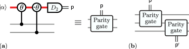
Figure 1: (a) Circuit to measure the parity of two qubits. The CRs are $\pm\theta$. (b) Two parity gates combined to measure the Pauli operators $ZZI$ and $IZZ$.

It can be seen that this circuit is a parity gate when we consider its effect on the input state $|\psi_{\text{in}}\rangle=\bigl{(}a_{0}|00\rangle+a_{1}|01\rangle+a_{2}|10\rangle+a_{3}|11\rangle\bigr{)}|\alpha\rangle$, where $|\alpha\rangle$ is a coherent bus mode. The effect of the CRs is to apply a phase to the coherent beam if our data qubit is $|1\rangle$ and leave it alone otherwise: $\bigl{(}a|0\rangle+b|1\rangle\bigr{)}|\alpha\rangle\to a|0\rangle|\alpha\rangle+b|1\rangle|\alpha e^{i\theta}\rangle$. Before the detector $D_{2}$ in Fig. 1a, the state $|\psi_{\text{in}}\rangle$ is $\bigl{(}a_{0}|00\rangle+a_{3}|11\rangle\bigr{)}|\alpha\rangle+a_{1}|01\rangle|\alpha e^{-i\theta}\rangle+a_{2}|10\rangle|\alpha e^{i\theta}\rangle$. When $D_{2}$ is a homodyne detection along the $x$-quadrature we are able to distinguish $a_{0}|00\rangle+a_{3}|11\rangle$ from $a_{1}|01\rangle+a_{2}|10\rangle$, since a homodyne measurement of $|\alpha\rangle$ along the $x$-quadrature is equivalent to the projection $\langle x|\alpha\rangle$. That is, $|\alpha e^{\pm i\theta}\rangle$ are indistinguishable when we homodyne detect along the $x$-quadrature. This is the basis of the CNOT shown in Nemoto04 .

With two parity gates we can measure the Pauli operators $ZZI$ and $IZZ$. That is, one parity gate is applied to qubits 1 and 2 to measure $ZZI$ while the second parity gate is applied to qubits 2 and 3 to measure $IZZ$, as shown in Fig. 1b. The state before the application of the parity gates is $|\overline{\psi}_{\text{in}}\rangle=\bigl{(}c_{0}|000\rangle+c_{1}|111\rangle\bigr{)}|\alpha\rangle|\alpha\rangle$. There are four cases to consider: no error, $|\overline{\psi}_{\text{in}}\rangle$; an error on qubit 1, $XII|\overline{\psi}_{\text{in}}\rangle$; an error on qubit 2, $IXI|\overline{\psi}_{\text{in}}\rangle$; an error on qubit 3, $IIX|\overline{\psi}_{\text{in}}\rangle$. We can see what the effect of a bit flip error on each of the modes is by considering the state $|abc\rangle|\alpha\rangle|\alpha\rangle$, where $a,b,c\in\{0,1\}$. Directly before homodyne detection in Fig. 1b $|abc\rangle|\alpha\rangle|\alpha\rangle$ becomes $|abc\rangle|\alpha e^{i(a-b)\theta}\rangle|\alpha e^{i(c-b)\theta}\rangle$. When we measure the probe states to be $|\alpha e^{\pm im\theta}\rangle|\alpha e^{\pm in\theta}\rangle$, where $m,n\in\{0,\pm 1\}$, we know whether there was no error ($m,n=0$) or a one bit flip error, the location of the bit flip also being identified by the values of $m$ and $n$. Similar methods can be applied to measure the stabilizer operators for Shor’s 9-qubit code. The natural question that arises is: can we use techniques similar to those above to measure the syndromes for an arbitrary stabilizer code?

Larger codes — As a concrete example, consider the $[[7,1,3]]$ stabilizer code Steane . This code can correct a single arbitrary quantum error in any of the 7 qubits, and it has been used extensively in studies of fault-tolerance in quantum computers due to the fact that it allows for simple constructions of fault-tolerant encoded gates Got98 . In order to detect which error has corrupted the data, one must measure six multiqubit Pauli operators which, up to qubit permutations and local unitaries, are equivalent to the Pauli operator $ZZZZ$, or the measurement of only the parity of 4 qubits. For an arbitrary stabilizer code, various multiqubit Pauli operator must be measured, each of which is always equivalent to a measurement of only the parity of a subset of qubits, thus it is sufficient to consider only multiqubit parity measurements in order to perform quantum error correction with stabilizer codes.

Single Coherent State Pulse — In order to measure $ZZZZ$ with CRs, we can start with the encoded state $\bigl{(}c_{0}|0_{L}\rangle+c_{1}|1_{L}\rangle\bigr{)}|\alpha\rangle$, and design a circuit that gives us $|\alpha_{1}\rangle$ when there was no error (even parity) and $|\alpha_{2}\rangle$ when there was an error (odd parity), where $\alpha_{1}\neq\alpha_{2}$.

Ideally we would want to do this with just one coherent probe beam, four CRs and a single homodyne detection, following a direct analogy with the circuit depicted in Fig. 1a. However this is not possible. The best we can do is have some even states go to $|\alpha\rangle$ and the rest go to $|\alpha e^{\pm 2i\theta}\rangle$ while the odd states go to $|\alpha e^{\pm i\theta}\rangle$. The circuit that performs this is shown in Fig. 2a.

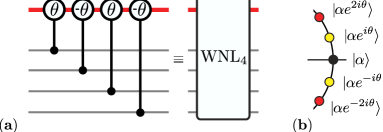
Figure 2: (a) First attempt at using CRs to measure the parity of four qubits with a single strong coherent probe. (b) Position of phase space peaks corresponding to the state of the coherent probe beam. Yellow circles correspond to odd states while red and black circles correspond to even states.

Notice that in phase space we would have five points – three for the even states ($|\alpha\rangle,|\alpha e^{\pm 2i\theta}\rangle$) and two for the odd states ($|\alpha e^{\pm i\theta}\rangle$) – as can be seen in Fig. 2b. If we were to homodyne detect the probe beam at this stage, we would partially decode our encoded state $c_{0}|0_{L}\rangle+c_{1}|1_{L}\rangle$ since we can distinguish the state $|\alpha\rangle$ from $|\alpha e^{\pm 2i\theta}\rangle$. The problem now becomes determining what operations must be done before we homodyne detect so that we only distinguish between states of different parity in the first four qubits, and nothing more. It turns out that either homodyne or photon number detection can be used, depending on the operations applied before the measurement.

Photon number measurement — If we incorporate displacements along with Fig. 2a we can take the five points in phase space to just three. Displacements of a state can be easily implemented by mixing the state with a large coherent state on a weak beam splitter, the size of the coherent states amplitude and beam splitter reflectivity deciding the displacement Displ . If we have three displacements and three applications of Fig. 2a, as in Fig. 3a, we find that $|\text{odd}\rangle\to|-4\alpha\sin^{2}(\theta/2)(2\sin^{2}(\theta)+\cos(\theta))\rangle$ and $|\text{even}\rangle\to|\pm 2\alpha\sin^{2}(\theta)(2\cos(\theta)-1)\rangle$, as depicted in Fig. 3b. The displacements that accomplish this are $D(\beta_{1})=D(-4\alpha\cos^{2}(\theta/2)\bigl{(}2\cos(\theta)-1\bigr{)})$, $D(\beta_{2})=D(\alpha\bigl{(}1+2\cos(\theta)+2\cos(3\theta)\bigr{)})$ and $D(\beta_{3})=D(\alpha(\cos(2\theta)-\cos(3\theta)-\cos(\theta)-1)$.

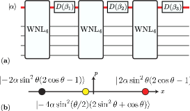
Figure 3: (a) CRs used to measure the parity of four qubits with a photon number detection. (b) Position of phase space peaks corresponding to the state of the coherent probe beam.

Notice that the red and black circle in the Fig. 3b are equidistant from the p-axis. We can thus perform a photon number measurement on the probe beam to determine whether we had an odd or even state. In order for a photon number measurement to distinguish the odd from even states we require $\alpha\theta^{2}\gg 1/\sqrt{3}$.

We can use this method to measure the parity for a state of any size. If we have $n$ qubits then we can have at best $n+1$ points in phase space, using the $\theta,-\theta,\theta,-\theta$ pattern for the CRs shown in Fig. 2a. Using displacements and a photon number detector we are able to measure the parity. In general, if $n$ is even we need $n-1$ displacements and $n^{2}-n$ CRs with a photon number measurement. When $n$ is odd, after the application of the circuit analogous to Fig. 2a of size $n$, we will have the point $|\alpha e^{i(2n-1)\theta}\rangle$ in phase space without the point $|\alpha e^{-i(2n-1)\theta}\rangle$. So we need an extra displacement to move the non-symmetric point. If $n$ is odd we need $n$ displacements and $n^{2}$ CRs with a photon number measurement.

For this method to work we need the use of a number discriminating photo-detector. In practice it is well known that homodyne detection is much more precise than number discriminating photo-detectors. For this reason, we describe how to measure a Pauli operator using homodyne detection.

Homodyne detection — Consider the $ZZZZ$ case again. After applying Fig. 2a we have five points in phase space. Ideally we want $|\alpha\rangle$ and $|\alpha e^{\pm 2i\theta}\rangle$ to become one point in phase space, say $R_{1}+iR_{2}$, and $|\alpha e^{\pm i\theta}\rangle$ to become one point, say $R_{3}+iR_{4}$. If this was possible then homodyne detection could be used. This can be done with five displacements and six applications of Fig. 2a, requiring 10 simultaneous equations to be solved. Without loss of generality we set $R_{2}=R_{4}=R_{1}=0$. The equations to be solved are $e^{4i\beta\theta}A+e^{3i\beta\theta}B+e^{2i\beta\theta}C+e^{i\beta\theta}D+E=e^{-i\beta\theta}\alpha_{\beta}-e^{5i\beta\theta}$, where $\alpha_{0,\pm 2}=0$ and $\alpha_{\pm 1}=R_{3}$.

After solving these equations we find that $A$, $B$, $C$, $D$ and $E$ scale as $-R_{3}/\theta^{4}$. We are free to choose the distance between the origin and $R_{3}$ to be arbitrarily large, at the expense of using arbitrarily large displacements. We can also use the above method to distinguish the parity of any given state of $n$ qubits. If we have $n$ qubits we have $n+1$ points in phase space, using a circuit similar to Fig. 2a. In order to distinguish the parity we need $n+1$ displacements and $n(n+2)$ CRs.

Fault-Tolerance — These two methods to measure weight $n$ Pauli operators cannot be used for fault-tolerant quantum computation. If there is an error on the coherent probe mode during one of the CRs, say photon loss, it would be transferred to a phase error in each of the physical qubits it interacts with afterwards – that is, a single fault can cause a number of errors which is greater than the number of errors the code can correct. For this reason we now look at measuring the syndromes of stabilizers fault-tolerantly.

Shor Shor96 first described how to fault-tolerantly measure the generators of the stabilizer group of a quantum error correcting code using ancilla GHZ states $\bigl{(}|0\rangle^{\otimes n}+|1\rangle^{\otimes n}\bigr{)}/\sqrt{2}$, CNOT’s and Hadamards. For example, in order to measure the Pauli operator $ZZZZ$ (which is equivalent to measuring the parity of 4 qubits and nothing else), we would use the circuit shown in Fig. 4a.

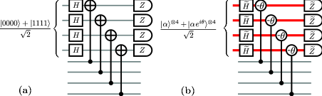
Figure 4: (a) Circuit for the measurement of the parity of four qubits Shor96 . (b) Same circuit modified to use coherent states and CRs.

To fault-tolerantly measure the stabilizer group generators of a QEC with CRs we make three modifications to Fig. 4a. First, instead of using $|0\rangle$ and $|1\rangle$ for the ancilla, we use the coherent states $|\alpha\rangle$ and $|\alpha e^{i\theta}\rangle$, respectively. In that case, the ancilla GHZ state becomes $\bigl{(}|\alpha\rangle^{\otimes n}+|\alpha e^{i\theta}\rangle^{\otimes n}\bigr{)}/\sqrt{2}$. Second, we replace the CNOT’s with CRs, which will cause a phase shift if the physical state is $|1\rangle$ and do nothing otherwise, i.e. $|1\rangle|\alpha\rangle\to|1\rangle|\alpha e^{-i\theta}\rangle$ and $|1\rangle|\alpha e^{i\theta}\rangle\to|1\rangle|\alpha\rangle$. We also need to replace the Hadamards with some quantum operation ${\widetilde{H}}$ which will perform the mapping ${\widetilde{H}}|\alpha\rangle\approx\bigl{(}|\alpha\rangle+|\alpha e^{i\theta}\rangle\bigr{)}/\sqrt{2}$ and ${\widetilde{H}}|\alpha e^{i\theta}\rangle\approx\bigl{(}|\alpha\rangle-|\alpha e^{i\theta}\rangle\bigr{)}/\sqrt{2}$. Third, we replace the qubit measurements with some sort of optical measurement that distinguishes between $|\alpha\rangle$ and $|\alpha e^{\pm i\theta}\rangle$ but not between $|\alpha e^{i\theta}\rangle$ and $|\alpha e^{-i\theta}\rangle$ – this is what we call ${\widetilde{Z}}$ measurement. This new circuit is depicted in Fig. 4b.

The ${\widetilde{Z}}$ measurements can be performed directly by homodyne detection, or by displacements followed by photon counting detectors – in both cases, using techniques outlined earlier in this paper. What remains to be specified is the preparation of the coherent cat state $(|\alpha\rangle^{\otimes n}+|\alpha e^{i\theta}\rangle^{\otimes n})/\sqrt{2}$ and the implementation of the ${\widetilde{H}}$ operation. One solution for the cat state preparation is to use one bit teleportations Zhou00 which translate states from the $|0\rangle/|1\rangle$ basis to the $|\alpha\rangle/|\alpha e^{\pm i\theta}\rangle$ basis. Preparation of the cat state is done by using the one bit teleportation in Fig. 5a to prepare $|\sqrt{n}\alpha\rangle+|\sqrt{n}\alpha e^{i\theta}\rangle$ from the state $\bigl{(}|0\rangle+|1\rangle\bigr{)}/\sqrt{2}$ and the coherent state $|\sqrt{n}\alpha\rangle$, and then sending this state into an $n$-port symmetric beam-splitter Gilchrist04 ; Ralph03 . In principle, we are required to correct the state before the beam-splitter by applying the transformation ${\widetilde{Z}}$ such that ${\widetilde{Z}}|\alpha\rangle\approx|\alpha\rangle$ while ${\widetilde{Z}}|\alpha e^{i\theta}\rangle\approx-|\alpha e^{i\theta}\rangle$. However, we can avoid explicitly applying this transformation by keeping track of this necessary correction – what is called the Pauli frame PauliFrame – and compensating for it in subsequent measurements. Similarly, to perform the ${\widetilde{H}}$ (the approximate Hadamard on coherent state logic) we first use Fig. 5b to teleport the quantum state from the bus to a qubit, then perform the Hadamard transformation and finally teleport back to the coherent state logic using the circuit shown in Fig. 5a.

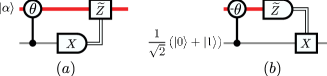
Figure 5: Approximate one bit teleportation protocols Zhou00 using CRs. The measurement dependent Pauli corrections need not be performed, as discussed in the body of the paper.

These teleportations, when performed back-to-back to teleport a qubit state to another qubit, can also be used as leakage reduction units to reduce leakage faults to regular faults AT07 .

The resources required to measure a weight $n$ Pauli operator are $3n+1$ CRs, $n+1$ ancillary qubits, $2n$ ${\widetilde{Z}}$ measurements and $n+1$ qubit measurements.

Noisy ancillas — If the probability of error at each gate is bounded by $\epsilon$, transversal operations and encoding can ensure that the probability of an uncorrectable error is $O(\epsilon^{2})$ instead of $O(\epsilon)$. An error during cat state preparation may lead to correlated $X$-like errors in the cat state with probability $O(\epsilon)$, which can lead to uncorrectable errors in the encoded data during the measurement of the Pauli operator, thus defeating the purpose of encoding the data for fault-tolerant quantum computation. In order to avoid this, one can verify the integrity of the cat state via non-destructive state measurement Pre97 ; AGP . When using CRs and coherent beam probes, this translates to preparing an extra copy of the cat state, which remains in coherent state logic, interacting with the qubit GHZ state transversally with controlled $-\theta$ rotations, and ${\widetilde{Z}}$ measuring each mode of the ancillary cat state. By performing classical error correction on the measurement outcomes, one can deduce the locations of $X$-like errors in either the GHZ state or the ancillary cat state. If the data is encoded in a code that can correct a single error, repeating this procedure with another ancillary cat state allows for the inference of which locations in the qubit GHZ state have $X$ errors with high enough probability to ensure uncorrectable errors are only introduced into the data with probability $O(\epsilon^{2})$ Pre97 , so that Pauli measurements with a verified ancilla can be used for fault-tolerant quantum computation. Overall, the overhead for each attempt of measuring a weight $n$ Pauli operator consists of $2(n+1)$ CRs, $2$ ancillary qubit preparations and measurements, and $2n$ ${\widetilde{Z}}$ measurements.

$Z$-like errors (including dephasing of coherent superpositions, one of the consequences of photon loss in the CRs) do not lead to errors in the encoded data, just errors in the outcome of the Pauli operator measurement. If error correction is to be performed, the Pauli operator measurement must be repeated $3$ times, and a majority vote of the outcomes is taken, in order to ensure that the measurement outcome is reliable Pre97 .

Some of the systematic errors in the probe beams, such as phase rotation or attenuation (also consequences of photon loss in the CRs), can be partially compensated for by additional linear-optics elements and by adjusting the ${\widetilde{Z}}$ measurements individually to minimize additional $X$ errors. Moreover, errors in the transversal operations during the preparation of the cat state are independent, and thus do not need special consideration during this verification stage – they do contribute to $\epsilon$, however, and are thus crucial for fault-tolerance threshold calculations.

Discussion — We have shown two schemes to measure the syndromes of an arbitrary weight $n$ Pauli operator. The first scheme uses a single strong coherent probe beam, a quadratic number of CRs, a linear number of coherent displacements, and a photon number or homodyne measurement – however, this scheme is not fault-tolerant. The second scheme we described is fault-tolerant, and the amount of resources scales linearly with the weight of the Pauli operator. This demonstrates how it is in principle possible to perform general fault-tolerant quantum computation in the qubus architecture. It is worth noting that we could have easily used controlled displacements in the place of CRs in the methods presented here.

Acknowledgments — We would like to thank P. Aliferis and R. Van Meter for valuable discussions. We are supported in part by NSERC, ARO, CIAR, MITACS, the Lazaridis Fellowship, MEXT in Japan and the EU project QAP.

References

- (1) D. Gottesman and I.L. Chuang, Nature 402, 390 (1999)
- (2) R. Raussendorf and H.J. Briegel, Phys. Rev. Lett. 86, 5188 (2001)
- (3) K. Nemoto and W.J. Munro, Phys. Rev. Lett. 93, 250502 (2004)
- (4) K. Nemoto and W.J. Munro, Phys. Lett. A 344, 104 (2005)
- (5) T. P. Spiller el. al. , New J. Phys. 8, 30 (2006)
- (6) F. Yamaguchi et. al, Phys. Rev. A 73, 060302 (2006).
- (7) A. Steane, Proc. Roy. Soc. London, Ser. A 452, 2551 (1996).
- (8) D. Gottesman, Phys. Rev. A 57, 127–137 (1998).
- (9) D.F. Walls and G.J. Milburn, Quantum Optics, (Springer-Verlag) 1994.
- (10) P.W. Shor, in Proceedings of the 37th Symposium on Foundations of Computer Science (IEEE, Los Alamitos, 1996), p. 56, quant-ph/9605011.
- (11) X. Zhou et. al, Phys. Rev. A 62, 052316 (2000).
- (12) A. Gilchrist et. al, J. Opt. B: Quantum Semiclass. Opt. 6, S828 (2004).
- (13) T.C. Ralph et. al, Phys. Rev. A 68, 042319 (2003).
- (14) A. M. Steane, Phys. Rev. A 68, 042322 (2003). E. Knill, Phys. Rev. A 71, 042322 (2005).
- (15) P. Aliferis and B. M. Terhal, Quant. Inf. Comp. 7, 139–156 (2007).
- (16) J. Preskill, Arxiv preprint quant-ph/9712048.
- (17) P. Aliferis et. al, Quant. Inf. Comp. 6(2), 97–165 (2006).