Dynamics of the Jaynes-Cummings and Rabi models: old wine in new bottles

Abstract

By using a wave packet approach, this paper reviews the Jaynes-Cummings model with and without the rotating wave approximation in a non-standard way. This gives new insight, not only of the two models themself, but of the rotating wave approximation as well. Expressing the models by field quadrature operators, instead of the typically used boson ladder operators, wave packet simulations are presented. Several known phenomena of these systems, such as collapse-rivivals, Rabi oscillation, squeezing and entanglement, are reviewed and explained in this new picture, either in an adiabatic or diabatic frame. The harmonic shape of the potential curves that the wave packets evolve on and the existance of a level crossing make these results interesting in a broader sense than only for models in quantum optics, especially in atomic and molecular physics.

I Introduction

Two fundamental models of quantum mechanics, presented in most introductory textbooks, are the two-level system and the harmonic oscillator. Combining these two into a bipartite system gives many interesting models, where two of the more studied ones are the Jaynes-Cummings (JC) model jc ; jc2 and the Rabi model rabi . The JC model was introduced for describing the interaction between a two-level atom and a quantized electromagnetic (EM) field, while the Rabi model was introduced for NMR systems. In this paper we will use the terminology of the JC model, a two-level atom and a quantized EM field, which, of course, does not restrict the results to such systems. The JC Hamiltonian is obtained from the Rabi one by simply imposing the rotating wave approximation RWA allen-eberly . There are, however, special cases where atomic selection rules make the JC model exact; the RWA terms naturally vanish selrule . In this approximation, exact analytical solutions exist, and, in spite the simplicity of the JC model, the dynamics have turned out to be very rich and complex, describing several physical phenomena. Among these are; Rabi oscillations rabi ; jcrabi , collapse-revivals cr , squeezing jcsqueez , atom-field entanglement entangle , non-classical states as Schrödinger cats cat and Fock states fock and anti-bunching jcab . The JC model originally thought of as a single atom, single field mode interaction, has shown to be applicable for several other types of systems, for example, trapped ions ion , Cooper-pair boxes cooper , ”flux” qubits flux and Josephson-junctions jj . With the experimental progress of some of the above mentioned systems, the coupling between the systems may be made very large, and the RWA breaks down so that only the Rabi model describes the dynamics correctly. As the number of excitations, field plus atom, is a constant of motion in the JC model, there are only two physically relevant parameters; detuning $\Delta$ between the atomic transition frequency $\Omega$ and the field mode frequency $\omega$ and atom-field coupling $g_{0}$. In the Rabi model, however, the number of excitations is not conserved and all three parameters are of importance. In general, the RWA is justified for small detunings $\Delta=\Omega-\omega$ and small ratios of the atom-field coupling divided by the atomic transition frequency, $g_{0}/\Omega$. In atom-field cavity systems, this ratio is typically of the order $g_{0}/\Omega\sim 10^{-7}-10^{-6}$, csys . Recently, cavity systems with very strong couplings have been discussed meystre . The ratio may also become order of magnitudes larger in solid state systems cooper , and the full Rabi Hamiltonian, including the virtual processes (also caller counter-rotating terms), must be considered. The neglection of the counter-rotating terms may have interesting physical consequencies on nonlocality and causality nlc . The effect of the RWA in other systems has been studied, and to mention a few, trapping of atoms by light trap , driven Rabi model drivjc , multi-level atoms and/or fields multi , the micromaser micro semiclassical Rabi models semi , transition between vibrational states in a water molecule water , dipolar molecules drivmol , light-matter interaction lightmat , electromagnetically and self induced transparency eit ; self and laser modified collisions lasercol .

Existence of analytical solutions for special cases of the Rabi model has been discussed rabiexsol . As no general simple solutions are known, much work has been devoted to various analytical approximate or numerical approaches, such as; perturbation theory pertur ; jcrwa ; rabiq ; pegg ; rabient ; pertrabi , path-integrals path , continued fractions confra , variational methods varm , coupled cluster methods ccm , displaced oscillators displace ; displace2 , approximated unitary transformed Rabi Hamiltonians unitrans and numerical studies adwp ; rabisqueez ; disq ; clsb ; num46 . The time-dependent Rabi Hamiltonian has been considered in timerabi , and a particular equivalence relation between the time-dependent JC and Rabi models was obtained. Interestingly, the Rabi model has shown to be chaotic chaos , contrary to the JC model jcchaos . The Bargmann representation barg , similar to our approach, has been considered for both the JC stig and the Rabi model rabibarg .

Using a different approach than the standard ones we discuss and review some of the work that has been done previously on the two models. The method used in this paper is a numerical wave packet propagation, which has been briefly applied to the Rabi model before adwp ; rabisqueez , but to the best of our knowledge not to the JC model. The system Hamiltonians are usually represented in the field creation and annihilation operators $a^{\dagger}$ and $a$, but here we instead work with the field quadrature operators $P$ and $Q$. As these obey the standard canonical commutation relations, the system is equivalent to a particle, with unit mass, moving in two coupled potentials, and the dynamics is given by the evolution of some initial wave packet. The idea of this paper is to give a deeper understanding of the JC and Rabi models by consider the wave packets evolving on these potential curves. Since the JC model is exactly solvable, it might seem unmotivated to use this numerical study. However, from the wave packet picture it is easy to understand some of the systems behaviours, and, additionally, due to the “graininess” of the cavity field most analytically obtained quantities predicted by the JC model are given as infinite sums lacking closed forms. As in related problems in molecular physics mol , it is often convenient to investigate the system in the diabatic or adiabatic basis adwp ; rabisqueez ; clsb ; adrabi . The proper basis used, depends on the system parameters and initial state. The critical evolution takes place close to level crossings between the two energy curves, and such a level crossing exists in both the JC and Rabi model. The two energy curves are given, in both models, by two displaced harmonic oscillators, and they are coupled by a constant coupling in both cases, while in the JC model there is an additional ”momentum” $P$ dependent coupling which gives rise to very different dynamics. The presence of the $P$ dependent coupling makes the wave packet evolution of the JC model less intuitive and more complex. Comparing the two models, combined with the knowledge of the validity regime of the RWA, one may interpret the consequences of this coupling term as well as other effects. In the intermediate regime, when one is neither in the adiabatic nor the diabatic validity regimes, a more detailed analysis is needed to understand the full evolution. This is only briefly mentioned in this paper.

The paper proceeds as the following. In the next section II we introduce the JC and Rabi Hamiltonians in their regular forms and also give them in the conjugate variable picture. In subsection II.3 the corresponding curve crossing problem is mentioned and how to approximate it as a Landau-Zener problem lz . The following section III, presents a background of an adiabatic approach, the two different bases, diabatic and adiabatic, are defined, and the approach is applied to both the JC and Rabi model. The validity of the adiabatic method is numerically studied in Sec. IV using the split operator procedure to calculate the fidelity. In Sec. V we present the numerical results of our studies. Several plots are shown to give a deeper insight of the dynamics and the phenomena are discussed from a wave packet point of view. Known interesting effects, such as entanglement, collapse-revivals, squeezing and Rabi oscillations, are especially studied. Finally we conclude the paper in sec. VI with a summery.

II The Jaynes-Cummings and Rabi models

II.1 Introducing the JC model with and without RWA

The simplest fully quantum mechanical model describing light-matter interaction, naturally considers one atom, with a single atomic transition, interacting with only one mode of the field. Such an approach leads to the JC or Rabi models. The single atom transition and single mode approximation relies on small or vanishing coupling elements between other levels scully . Thus, mathematically one is left with a two-level atom (spin-1/2 particle) coupled to a harmonic oscillator. For a dipole interaction, $H_{int}=\bar{d}\cdot\bar{E}/\hbar$, where $\bar{d}$ and $\bar{E}$ are the atomic dipole moment and electric field respectively, a microscopic derivation scully gives the Rabi Hamiltonian

$$H_{Rabi}=\hbar\omega\left(a^{\dagger}a+\frac{1}{2}\right)+\frac{\hbar\Omega}{2}\sigma_{z}+\hbar g_{0}\left(\sigma^{+}+\sigma^{-}\right)\left(a^{\dagger}+a\right).$$ (1)

Here, $a^{\dagger}$ ($a$) is the creation (annihilation) operator for the field mode; $a|n\rangle=\sqrt{n+1}|n+1\rangle$ ($a|n\rangle=\sqrt{n}|n-1\rangle$), the sigma operators are the standard Pauli matrices acting on the two-level atom; $\sigma_{z}|\pm\rangle=\pm|\pm\rangle$, $\sigma^{\pm}|\pm\rangle=|\mp\rangle$, $\sigma_{x}=\sigma^{+}+\sigma^{-}$ and $\sigma_{y}=-i\left(\sigma^{+}-\sigma^{-}\right)$, $\omega$ ($\Omega$) is the field (atomic transition) frequency and $g_{0}$ is the effective atom-field coupling. In deriving (1), the dipole approximation has been assumed, where the variation of the field is neglected on the atomic length scale, and the kinetic energy of the atom is omitted, valid for large and moderate temperatures effmass .

The interaction part contains four terms; $\sigma^{+}a^{\dagger}$ ($\sigma^{-}a$) simultaneous excitation (de-excitation) of the atom and field, and $\sigma^{+}a$ ($\sigma^{-}a^{\dagger}$) excitation of the atom by absorption of one photon (de-excitation of the atom by emission of one photon). In the Heisenberg picture, the operators evolve (free field and free atom case) as: $a(t)=a\exp(i\omega t)$, $a^{\dagger}(t)=a^{\dagger}\exp(-i\omega t)$ and $\sigma^{\pm}(t)=\sigma^{\pm}\exp(\pm i\Omega t)$. Thus, the interaction terms precess with either the frequencies $|\Omega-\omega|$ (energy conserving terms) or $\Omega+\omega$ (non energy conserving/counter rotating terms). Most often $|\Omega-\omega|\ll\Omega+\omega$ and the fast oscillating terms are rejected from the Hamiltonian, resulting in the Jaynes-Cummings Hamiltonian

$$H_{JC}=\hbar\omega\left(a^{\dagger}a+\frac{1}{2}\right)+\frac{\hbar\Omega}{2}\sigma_{z}+\hbar g_{0}\left(\sigma^{+}a+\sigma^{-}a^{\dagger}\right).$$ (2)

However, for a large atom-field detuing (but still within the atomic two-level and single mode approximations), the above constrain may be violated and the non energy conserving terms can not be excluded. As mentioned in the introduction, also the ratio $g_{0}/\Omega$ is important for the validity of the above RWA. The two conditions for the RWA must in general be met simultaneously, meaning that near resonant interaction does not gurantee validity of the RWA if not $g_{0}<\Omega$, and vice versa.

II.2 The models in the conjugate variable picture

The JC model is usually given and solved within the ”number”-basis of the field $\{|n\rangle|\pm\rangle\}$. Here, however, we will work in the conjugate variable basis of the field. We introduce the conjugate variables $P$ and $Q$ related to the creation/annihilation operators as

$$\begin{array}[]{l}P=i\sqrt{\frac{\hbar\omega}{2}}\left(a^{\dagger}-a\right),\\ \\ Q=\sqrt{\frac{\hbar}{2\omega}}\left(a^{\dagger}+a\right).\end{array}$$ (3)

In the transformed basis the Rabi (1) and the JC (2) Hamiltonians read

$${H_{Rabi}=\frac{P^{2}}{2}+\frac{\omega^{2}}{2}Q^{2}+\left[\begin{array}[]{cc}\displaystyle{\frac{\hbar\Omega}{2}}&g_{0}\sqrt{2\hbar\omega}Q\\ g_{0}\sqrt{2\hbar\omega}Q&-\displaystyle{\frac{\hbar\Omega}{2}}\end{array}\right]},$$ (4)

$$\begin{array}[]{c}\displaystyle{H_{JC}=\frac{P^{2}}{2}+\frac{\omega^{2}}{2}Q^{2}}\\ \\ \displaystyle{+\left[\begin{array}[]{cc}\displaystyle{\frac{\hbar\Omega}{2}}&\displaystyle{g_{0}\sqrt{\frac{\hbar}{2}}\left(\sqrt{\omega}Q+i\frac{P}{\sqrt{\omega}}\right)}\\ \displaystyle{g_{0}\sqrt{\frac{\hbar}{2}}\left(\sqrt{\omega}Q-i\hbar\frac{P}{\sqrt{\omega}}\right)}&-\displaystyle{\frac{\hbar\Omega}{2}}\end{array}\right]}.\end{array}$$ (5)

Relating $P$ and $Q$ as momentum and position operators respectively, the above Hamiltonians can be interpreted as a two-level particle, with quantized position and momentum, confined in a harmonic trap and interacting with a ”classical” field with mode ”variations” $g(Q,P)\sim Q$ or $g(Q,P)\sim\left(Q+i\frac{P}{\omega}\right)$. The Rabi Hamiltonian could be obtained, for example, by considering a harmonically trapped two-level atom driven by a classical field, whose wave length is much longer than the extent of the atomic wave packet in the trap and with a node at the centre $Q=0$. In other words, there is a direct connection between the above example of a trapped atom and an atom interacting with a quantized field. Relating the JC Hamiltonian to similar systems is less trivial, since the atom-field coupling is momentum dependent.

II.3 The corresponding curve crossing problem

The structure of the Rabi Hamiltonian (4) is more easily seen by applying the unitary transformation $U=\frac{1}{\sqrt{2}}\left(\sigma_{x}+\sigma_{z}\right)$, giving the transformed Hamiltonian

$$\begin{array}[]{c}\displaystyle{\tilde{H}_{Rabi}=U^{\dagger}H_{Rabi}U=\frac{P^{2}}{2}+\frac{\omega^{2}}{2}Q^{2}}\\ \\ +\left[\begin{array}[]{cc}g_{0}\sqrt{2\hbar\omega}Q&\displaystyle{\frac{\hbar\Omega}{2}}\\ \displaystyle{\frac{\hbar\Omega}{2}}&-g_{0}\sqrt{2\hbar\omega}Q\end{array}\right].\end{array}$$ (6)

By completing the squares we may write the Hamiltonian as

$$\tilde{H}_{Rabi}\!=\!\frac{P^{2}}{2}+\left[\!\begin{array}[]{cc}V_{h}\left(\!Q\!+\!\sqrt{\frac{2\hbar}{\omega^{3}}}g_{0}\!\!\right)&\displaystyle{\frac{\hbar\Omega}{2}}\\ \displaystyle{\frac{\hbar\Omega}{2}}&V_{h}\left(\!Q\!-\!\sqrt{\frac{2\hbar}{\omega^{3}}}g_{0}\!\!\right)\end{array}\!\right]-\frac{\hbar g_{0}^{2}}{\omega},$$ (7)

where $V_{h}(x)=\omega^{2}x^{2}/2$ is the regular harmonic oscillator potential. Thus, it is seen that the problem is equivalent to the one of a particle moving in two coupled equally, but opposite, displaced harmonic potential curves. The two energy curves cross for $Q=0$, and the off diagonal coupling $\hbar\Omega/2$ results in an avoided crossing. As is well known; the main population transfer between two levels occurs close to the crossing. Here the distance between the curves relative to the coupling amplitude is the smallest. Therefor, in some situations the coupled dynamics may be considered only in the vicinity of the crossing. By linearizing the model around $Q=0$ we get

$$\tilde{H}_{Rabi}=\frac{P^{2}}{2}+\left[\begin{array}[]{cc}g_{0}\sqrt{2\hbar\omega}Q&\displaystyle{\frac{\hbar\Omega}{2}}\\ \displaystyle{\frac{\hbar\Omega}{2}}&-g_{0}\sqrt{2\hbar\omega}Q\end{array}\right].$$ (8)

If the wave packet is well localized (the characteristic width of the wave packet $\Delta_{Q}$ is small compared to variations of the harmonic potential), the ”momentum” and ”position” may be replaced by its classical counterparts at the crossing; $P\rightarrow v$ and $Q\rightarrow vT$, where $T$ is the time. Neglecting the constant terms, the Hamiltonian reduces to the one of the Landau-Zener model lz

$$\tilde{H}_{Rabi}=\left[\begin{array}[]{cc}\sqrt{2\hbar\omega}g_{0}vT&\displaystyle{\frac{\hbar\Omega}{2}}\\ \displaystyle{\frac{\hbar\Omega}{2}}&-\sqrt{2\hbar\omega}g_{0}vT\end{array}\right],$$ (9)

where the classical velocity $v$ will, of course, depend on the initial state of the system. The time dependent problem given by the Hamiltonian (9) is analytically solvable, with asymptotic solution for the population transfer to the other level given by

$$P_{LZ}=1-\exp\left(-\frac{\pi\Omega^{2}}{4\sqrt{2\hbar\omega}g_{0}v}\right).$$ (10)

The validity of this semiclassical model may be studied in a detailed way similar to the one in holthaus .

The same procedure may be applied to the JC Hamiltonian (5);

$$\tilde{H}_{JC}\!=\!\frac{P^{2}}{2}\!+\!\left[\!\begin{array}[]{cc}V_{h}\left(Q\!+\!\sqrt{\frac{\hbar}{2\omega^{3}}}g_{0}\!\!\right)&\displaystyle{\frac{\hbar\Omega}{2}\!-\!ig_{0}\sqrt{\frac{\hbar}{2\omega}}P}\\ \displaystyle{\frac{\hbar\Omega}{2}\!+\!ig_{0}\sqrt{\frac{\hbar}{2\omega}}P}&V_{h}\!\left(\!Q\!-\!\sqrt{\frac{\hbar}{2\omega^{3}}}g_{0}\!\!\right)\end{array}\!\right]\!-\!\frac{\hbar g_{0}^{2}}{4\omega}.$$ (11)

One notes that the displaced oscillators are shifted half the amount as in the Rabi Hamiltonian, and that there is an additional $P$-dependent coupling of the oscillators. As the RWA implies that non energy conserving terms are omitted, it follows that the number of excitations is conserved. Thus, $N=\frac{P^{2}}{2\omega}+\frac{\omega}{2}Q^{2}+\frac{1}{2}\sigma_{z}$ commutes with $H_{JC}$, and one may work in a rotating frame with respect to $N$. Applying the same unitary operator to the new interaction picture Hamiltonian $H^{\prime}_{JC}=H_{JC}-\hbar\omega N$, one finds

$$\tilde{H}^{\prime}_{JC}=\left[\begin{array}[]{cc}\displaystyle{g_{0}\sqrt{\frac{\hbar\omega}{2}}Q}&\displaystyle{\frac{\hbar\Delta}{2}-ig_{0}\sqrt{\frac{\hbar}{2\omega}}P}\\ \\ \displaystyle{\frac{\hbar\Delta}{2}+ig_{0}\sqrt{\frac{\hbar}{2\omega}}P}&\displaystyle{-g_{0}\sqrt{\frac{\hbar\omega}{2}}Q}\end{array}\right]$$ (12)

The energy transfer between the atom and the field in the JC model is give by $\tilde{H}^{\prime}_{JC}$, and from (12) we note the similarities with the Landau-Zener problem but with the addition “momentum” dependent coupling. An interesting observation is that if the wave packet approaches the curve crossing with a high momentum, an adiabatic evolution is still possible due to the large curve couplings. At the one hand, “velocity” determines the steepness of the crossing curves, but on the other is also determines level separation close to the coupling. This peculiar curve crossing model is, of course, an artifact of the RWA, but none the less it may give insight into other related systems, for example atomic and molecular scattering processes ccross .

III The adiabatic approach

III.1 Review of the adiabatic principle

The concept of adiabaticity is widely used in a variety of physical and chemical systems, while, what is known as the adiabatic theorem adth is only stated for time-dependent Hamiltonian systems. Non the less, the principle may be transferred to other systems where the dynamics is governed by the evolution of some initial state adgen . Here we review the results of jonas1 , and apply it to our models in the following subsections.

Given a Hamiltonian of the form

$$H=\frac{p^{2}}{2m}+V(x)+\left[\begin{array}[]{cc}\displaystyle{\frac{\hbar\Delta(x,p)}{2}}&\hbar g(x,p)\\ \hbar g(x,p)&-\displaystyle{\frac{\hbar\Delta(x,p)}{2}}\end{array}\right].$$ (13)

The diagonal elements are often refereed to as detuning, and for simplicity they will be taken constant $\Delta(x,p)=\Delta$, and the off diagonal ones are level couplings. We introduce the parameter $\theta$ accordingly

$$\tan 2\theta=\frac{2g(x,p)}{\Delta},$$ (14)

such that the unitary transformation

$$U=\left[\begin{array}[]{cc}\cos\theta&-\sin\theta\\ \sin\theta&\cos\theta\end{array}\right]$$ (15)

diagonalizes the last term of the Hamiltonian (13) with corresponding eigenvalues

$$\lambda_{\pm}=\pm\lambda=\pm\hbar\sqrt{\left(\frac{\Delta}{2}\right)^{2}+g^{2}(x,p)},$$ (16)

and eigenstates, defining the new adiabatic basis states,

$$|\uparrow\rangle=\left[\begin{array}[]{c}\cos\theta\\ \sin\theta\end{array}\right],\hskip 28.45274pt|\downarrow\rangle=\left[\begin{array}[]{c}-\sin\theta\\ \cos\theta\end{array}\right].$$ (17)

However, since in general $[p,g(x,p)]\neq 0$ and $[V(x),g(x,p)]\neq 0$, the new Hamiltonian will not be diagonal. Introducing the two functions $f=\cos\theta$ and $h=\sin\theta$, and using the identity

$$U^{\dagger}pU=p-\sigma_{y}\hbar\partial\theta,$$ (18)

where

$$\partial\theta\equiv\frac{\partial\theta}{\partial x}$$ (19)

the transformed Hamiltonian takes the form

$$\tilde{H}=\tilde{H}_{ad}+\tilde{H}_{cor},$$ (20)

with the adiabatic part

$$\tilde{H}_{ad}=\frac{p^{2}}{2m}+(\hbar\partial\theta)^{2}+fV(x)f+hV(x)h+\left[\begin{array}[]{cc}\lambda&0\\ 0&-\lambda\end{array}\right]$$ (21)

and the correction part

$$\begin{array}[]{lll}\tilde{H}_{cor}&=&\frac{1}{2m}\left[\begin{array}[]{cc}0&\hbar^{2}\partial^{2}\theta-2i\hbar(\partial\theta)p\\ -\hbar^{2}\partial^{2}\theta+2i\hbar(\partial\theta)p&0\end{array}\right]\\ \\ &&+\left(fV(x)h-hV(x)f\right)i\sigma_{y}.\end{array}$$ (22)

Note that if $V(x)$ commutes with $g(x,p)$ we have $fV(x)f+hV(x)h=V(x)$ and $fV(x)h-hV(x)f=0$. As it will turn out, this will be the case in our models, and we therefor assume commutability.

An adiabatic evolution is obtained if the dynamics is dominated by the diagonal adiabatic Hamiltonian $H_{ad}$ of (20), while $H_{cor}$ only slightly affects the propagation. Clearly, this depends on the smoothness of $\theta$ and the momentum $p$, but also on the wave packet shape. Using the definition of the angle parameter (14) we find

$$\begin{array}[]{l}\displaystyle{\partial\theta=\frac{\Delta\partial g}{\Delta^{2}+4g^{2}}},\\ \\ \displaystyle{\partial^{2}\theta=\frac{\Delta\left(\partial^{2}g\left(\Delta^{2}+4g^{2}\right)-8g(\partial g)^{2}\right)}{\left(\Delta^{2}+4g^{2}\right)^{2}}}.\end{array}$$ (23)

Under the adiabatic approximation, the state is evolved on the adiabatic energy curves $\varepsilon_{\pm}=V\pm\lambda$ according to

$$\begin{array}[]{lll}\Psi^{ad}(x,t)&=&\exp\left[-i\left(\frac{p^{2}}{2m}+\varepsilon_{+}\right)t\right]\psi_{\uparrow}^{ad}(x,0)|\uparrow\rangle\\ \\ &&+\exp\left[-i\left(\frac{p^{2}}{2m}-\varepsilon_{-}\right)t\right]\psi_{\downarrow}^{ad}(x,0)|\downarrow\rangle.\end{array}$$ (24)

In the opposite limit, the non-adiabatic case, the evolution takes place on the diabatic energy curves (also called bare energies), defined by the diagonal elements of the Hamiltonian. Note, though, that the diabatic energies depend on the basis used.

III.2 Application to the JC model

Before proceeding, we introduce scaled dimensionless variables. We scale energies with the photon energy $\hbar\omega$, ”lengths” $Q$ by $\sqrt{\hbar/\omega}$ and time by $\omega^{-1}$:

$$\begin{array}[]{lll}\displaystyle{q=\sqrt{\frac{\omega}{\hbar}}Q},&&t=\omega T\\ \\ \displaystyle{\tilde{\Omega}=\frac{\Omega}{\omega}},&&\displaystyle{\tilde{g}_{0}=\frac{g_{0}}{\omega}}.\end{array}$$ (25)

For convenience we drop the tildes $\sim$ on the last two scaled variables.

Introduced in the subsection II.3, it is convenient to work in an interaction picture with respect to excitation operator,

$$H^{\prime}_{JC}=H_{JC}-N=\left[\begin{array}[]{cc}\displaystyle{\frac{\Delta}{2}}&\displaystyle{g_{0}\frac{1}{\sqrt{2}}\left(q+ip\right)}\\ \\ \displaystyle{g_{0}\frac{1}{\sqrt{2}}\left(q-ip\right)}&\displaystyle{-\frac{\Delta}{2}}\end{array}\right],$$ (26)

with the detuning $\Delta=\Omega-1$. As the interaction picture Hamiltonian is lacking the kinetic energy operator and the ”external potential”, the correction $H_{cor}$ to the adiabatic Hamiltonian vanishes. The eigenstates are

$$\begin{array}[]{l}|\uparrow\rangle_{n}=\cos\theta\psi_{n-1}(q)|+\rangle+\sin\theta\psi_{n}(q)|-\rangle,\\ \\ |\downarrow\rangle_{n}=\sin\theta\psi_{n-1}(q)|+\rangle-\cos\theta\psi_{n}(q)|-\rangle,\end{array}$$ (27)

where

$$\tan 2\theta=\frac{2g_{0}\sqrt{n}}{\Delta},$$ (28)

and $\psi_{n}(q)$ is the $n$th eigenfunctions to the harmonic oscillator. As $q\pm ip$ act as raising and lowering operators, the diagonaliced Hamiltonian in the original picture and within the $n$th block reads

$$H_{JC}=\frac{p^{2}}{2}+\frac{q^{2}}{2}+\frac{1}{2}\sigma_{z}\pm\sqrt{\left(\frac{\Delta}{2}\right)^{2}+g_{0}^{2}n}.$$ (29)

Thus, the eigenvalues are

$${E_{\pm}(n)=\left(n+\frac{1}{2}\right)\pm\sqrt{\left(\frac{\Delta}{2}\right)^{2}+g_{0}^{2}n}}.$$ (30)

The ”adiabatic limit” in the JC model is generally taken as $\Delta\gg g_{0}\sqrt{n}$. It has been shown jonas1 that this limit governs adiabatic evolution, but that this is not the only possibility. Expanding the solutions (27) and (30) to first order in $g_{0}\sqrt{n}/\Delta$ reproduce the familiar results from ”adiabatic elimination” in the JC model adel .

III.3 Application to the Rabi model

Applying the above method to the Rabi Hamiltonian (4) give the adiabatic Hamiltonian

$$H_{ad}=\frac{p^{2}}{2}+V_{\pm}(q),$$ (31)

where

$$V_{\pm}(q)=\frac{q^{2}}{2}+\frac{2\Omega^{2}g_{0}^{2}}{\left(\Omega^{2}+2g_{0}^{2}q^{2}\right)^{2}}\pm\sqrt{\left(\frac{\Omega}{2}\right)^{2}+2g_{0}^{2}q^{2}}$$ (32)

and the corresponding adiabatic states given in (17). In the limit $\Omega\rightarrow 0$, the adiabatic correction vanishes and the problem is analytically solvable, since (31) becomes identical to two displaced disconnected harmonic oscillators.

The standard way of defining an adiabaticity criteria is by letting the ”distance” between the adiabatic energies become much larger than the amplitude of the off-diagonal couplings adth . In our particular model, we explicitly have

$$\begin{array}[]{l}\displaystyle{\partial\theta=\frac{\Omega g_{0}\sqrt{2}}{\Omega^{2}+2g_{0}^{2}q^{2}}},\\ \\ \displaystyle{\partial^{2}\theta=-\frac{4\Omega g_{0}^{3}\sqrt{2}q}{\left(\Omega^{2}+2g_{0}^{2}q^{2}\right)^{2}}}.\end{array}$$ (33)

For smooth angles $\theta$, the main non-adiabatic contribution will come from the term $2(\partial\theta)p$, where a large $p$ is obtained by having a large $\langle n\rangle$ which is known to violate adiabaticity. We directly note that the standard adiabatic limit $\Omega\gg g_{0}$ gives a small coupling. However, we also note that if $q^{2}\gg\left(\sqrt{2}g_{0}\Omega-\Omega^{2}\right)/2g_{0}^{2}$, an adiabatic evolution is obtained, which is intuitive as we are far from the curve crossing. It is instructive to analyze the diabatic and adiabatic energy curves for different sets of parameters which is shown in fig. 1. Note that the diabatic energies are just the displaced harmonic oscillators $V_{h}(q\pm\sqrt{2}g_{0})$. In (a), the atomic frequency $\Omega$ is larger than the coupling and we have in this situation the regular adiabatic limit. In (b)-(d) $\Omega$ is smaller or equal to $g_{0}$ and an adiabatic evolution is only expected when the wave packet is well localized at positions $|q|\gg 0$. We note how the barrier in the middle at $q=0$ of the adiabatic curves is lower, but wider, for increasing $\Omega$. This peak will most likely govern a non-adiabatic transition between the adiabatic states. This again, indicates that adiabatic evolution is only obtained far from the crossing in these situations. For large enough $|q|$ the adiabatic and diabatic states coincide for any parameters. When $\Omega/g_{0}$ is small, a large $|q|$ is needed to assure adiabaticity, while a large $\Omega/g_{0}$ induces adiabaticity for all ”positions” $q$. Thus, since the states we propagate will most often pass through the level crossing we conclude that for $\Omega>g_{0}$ the behaviour may be understood from the evolution on the adiabatic energy curves, while for $\Omega<g_{0}$ it is better to use the diabtic curves.

For simplicity, the initial state will be given by the atom in its excited state and the field in some photon distribution, hence

$$\Psi(q,0)=\psi_{+}(q,0)|+\rangle=\psi_{+}(q,0)\left(\cos\theta|\uparrow\rangle-\sin\theta|\downarrow\rangle\right).$$ (34)

This limits the analysis, since more effects may be seen with other initial conditions, but that would greatly extend the leangth of the paper. For an initial Fock state, $a^{\dagger}a|n\rangle=n|n\rangle$, or coherent state, $a|\nu\rangle=\nu|\nu\rangle$, we have in $q$-representation respectively

$$\begin{array}[]{l}\displaystyle{\psi_{n}(q,0)=\frac{1}{\sqrt{2^{n}n!}}\left(\frac{1}{\pi}\right)^{1/4}\mathrm{H}_{n}(q)\mathrm{e}^{-\frac{q^{2}}{2}}},\\ \\ \displaystyle{\psi_{\nu}(q,0)=\left(\frac{1}{\pi}\right)^{1/4}\mathrm{e}^{-(\Im\nu)^{2}}\mathrm{e}^{-\frac{1}{2}\left(q-\sqrt{2}\nu\right)^{2}}},\end{array}$$ (35)

where $\mathrm{H}_{n}$ is the $n$th order Hermite polynomial. We note that for initial Fock states, adiabaticity is not expected if $\Omega<g_{0}$, since their wave functions are non-zero around $q=0$. However, for odd $n$ we have $\psi_{n}(q=0,0)=0$, but numerics indicate that adiabaticity is lost also for such states.

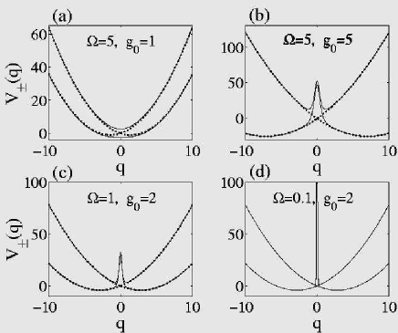
Figure 1: Solid lines display the adiabatic energy curves (32) for four different sets of dimensionless parameters indicated in the plots. The dotted lines show the corresponding displaced harmonic potentials $V_{h}(q\pm\sqrt{2}g_{0})$. Here the ”momentum” $p=1$.

IV Validity check of the adiabatic approximation

The validity of the adiabatic approximation is studied from a full wave packet simulation. The method used is the split operator procedure split , which relies on separation of the evolution operator into a momentum and position dependent one. The wave packet is either given in the $q$- or the $p$-representation, by a simple fast Fourier transform (FFT). The initial state of the field is given in eq. (34), and it will be propagated by, either the adiabatic Hamiltonian (31) or the full Hamiltonian (4). From the corresponding states, labelled $\Psi^{ad}(q,t)$ and $\Psi(q,t)$ respectively, we measure the validity of the approximation with the fidelity

$$F(t)=\sqrt{\left|\int\Psi^{*}(q,t)\Psi^{ad}(q,t)\,dq\right|}.$$ (36)

Numerical simulations indicate that a large detuning, $\Omega\ll 1$ or $\Omega\gg 1$, governs an adiabatic evolution. These limits are opposite to the one related to validity of the RWA. However, the limit $(g_{0}/\Omega)\rightarrow 0$ assures applicability of the adiabatic approximation and RWA. Non the less, there are parameter regimes where the adiabatic approximation is justified, while RWA breaks. Particularly, for a fixed ratio $g_{0}/\Omega$, the limits $\Omega\rightarrow\infty$ or $\Omega\rightarrow 0$ guarantee adiabaticity.

In fig. 2 we show the dependence of the fidelity (36), for an initial empty cavity (Fock state), on the coupling amplitude $g_{0}$ and time $t$. In the left plot $\Omega=2$ and in the right one $\Omega=0.5$, and it is clear that keeping $g_{0}/\Omega$ small results in an adiabatic evolution. The next plot, fig 3, gives the same, but now for an initial coherent state of the cavity field with an amplitude $\nu=4$. In (a) $\Omega=10$ and in (b) $\Omega=0.1$. The colour scale is the same for both figures. By lowering the amplitude $\nu$ the fidelity would be increased. It should be emphasised again that for a larger detuning between the mode and atomic transition frequency, one would also obtain a more adiabatic evolution.

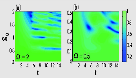
Figure 2: (Colour online)Plots of the fidelity (36), for an initial excited atom and empty cavity, as a function of scaled time $t$ and atom-field coupling $g_{0}$. In (a) the atom transition frequency is $\Omega=2$ and in (b) $\Omega=0.5$. The colourbar to the right displays the value of $F(t)$.

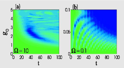
Figure 3: (Colour online) The same as fig. 2, but for an initial coherent state with $\langle n\rangle=|\nu|^{2}=16$. The atomic transition frequencies are $\Omega=10$ and $\Omega=0.1$. The colour scale is the same as in fig. 2.

V Numerical investigations

In this section we investigate in a non-standard way some of the more well-known phenomena predicted by the JC model. Wave packet propagation will be presented for both the JC and Rabi model. As mentioned in the introduction, one advantage of the method of using wave packet propagation is that it is valid for all parameter regimes. However, one should keep in mind that the adiabatic approximation is only valid within certain parameter regimes as seen in the previous section. The numerical results will be analyzed in terms of the wave packets propagating on the appropriate adiabatic or diabatic energy curves.

V.1 Rabi oscillations

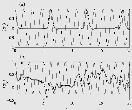
Figure 4: The figure shows the atomic inversion (Rabi oscillations) for an initial empty cavity and excited atom. Circles give the non-RWA results, while solid lines the RWA ones. In (a) $\Omega=0.2$ and $g_{0}=2$ and in (b) $\Omega=4$ and $g_{0}=2$.

Rabi oscillations rabi describes the periodic population swapping between some few internal levels, driven by an external ”field”. For the JC model, Rabi oscillations manifest themselves by population transfer between the upper and lower atomic state, equivalent to an energy transfer between the field and the atom. These oscillations are ”exact” when the field is initially in a Fock state and the systems are in resonance. Rabi oscillations have been measured in several JC type of systems jcrabi , and also theoretically studied for the Rabi model rabirabi . When the non energy conserving terms are included, the structure of the oscillations may be greatly affected. Figure 4 gives two examples where circles correspond to the Rabi model and solid line to the JC one. In (a) we have $\Omega<\omega,g_{0}$, while in (b) $\Omega>\omega,g_{0}$. The peaks of $\langle\sigma_{z}\rangle$ in fig. 4 (a) come with a period of $2\pi$ (in scaled units, where $\omega=1$). The adiabatic frame is no longer appropriate for giving an intuition of the behaviour, but instead one may consider the wave packets as evolving on the two displaced oscillators. For the Rabi model, the wave packet starts at the origin and then splits up into two parts, respectively propagating down the two displaced oscillators. After one classical period of oscillation the two packets return to their original positions and the interference gives rise to the peak. In the JC model, the wave packet will not split into two disconnected parts because of the $p$ dependent coupling which tend to bound the wave packet to the origin. Therefor, there is no collapse in the Rabi oscillations. In (b), the situation is adiabatic and since the adiabatic energy curves, fig. 1 (a), do not form two displaced oscillators, a collapse of the Rabi oscillations is not as clear as in (a) for the Rabi model. In fig. 5 (a) and (c) we show the amplitudes of the wave packets $\psi_{\pm}(q,t)$ corresponding to fig. 4 (a), while in fig. 5 (b) and (d) we display the same but for an initial Fock state with $n=2$ photons. The Rabi model wave packets are displayed in (a) and (b), while (c) and (d) show the wave packets for the regular JC model. Note that in (d) the wave packet either has two or three peaks depending on if the field contains 1 or 2 photons respectively. The imperfect revivals come from the weak coupling between the two oscillators, which induces the level splitting of the oscillators at $q=0$.

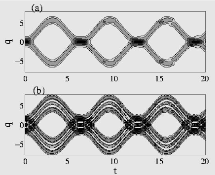
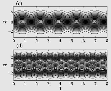
Figure 5: The absolute amplitudes of the wave packets corresponding to the previous fig. 4 (a) without RWA (a) and (b) and with RWA (c) and (d). In (a) and (c) the number of photons of the initial state is as in fig. 5 (a); $n=0$, while in (b) and (d) $n=2$.

Figure 6 gives the effect of the $p$ dependent coupling of the two displaced oscillators in the JC model. It shows the amplitudes $|\psi_{\pm}(q,t)|$ (upper plots) and $|\psi_{\uparrow,\downarrow}(q,t)|$ (lower plots), for the Rabi model with initial Fock state $|n=4\rangle$. The parameters are as in fig. 1 (d) and it is clear how the lower adiabatic wave packet slides down the displaced oscillators, while the upper adiabatic wave packet is squeezed at first. In the JC model, the wave packets would look very similar to those of fig. 5 (c) and (d), since we know that the population Rabi oscillates between the two Fock states $|n=4\rangle$ and $|n=5\rangle$. We can thus conclude that the spreading and squeezing of the wave packets in the Rabi model is due to the absence of the $p$ dependent coupling. This has been verified numerically by artificially neglecting the $p$ term from the JC model and a similar evolution as in the Rabi case is obtained. This effect of the $p$ term obviously holds for any initial Fock state, also for large photon numbers $n$, which has a broad wave packet. This may seem counterintuitive since for large $n$ the wave packet is non vanishing where the two energy curves are far apart and no coupling is expected to take part. However, as $n$ increases, the wave packet width also increases in momentum space and the $p$-coupling between the curves becomes stronger.

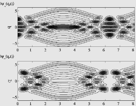
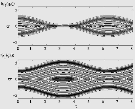
Figure 6: The four different absolute amplitudes for the Rabi model in the strong coupling regime corresponding to fig. 1 (a), $g_{0}=1$ and $\Omega=0.1$.

V.2 Collapse-revivals

One of the more interesting phenomenon of the JC model is the collapse-revival effect cr . This is a direct consequence of the ”graininess” of the field: Various parts of the state will Rabi oscillate with different frequencies, depending on the photon number $n$, leading to a collapse of various physical quantities, such as the atomic inversion $\langle\sigma_{z}\rangle$. However, after some particular time the parts may come back in phase and a revival occurs. Revivals for evolving wave packets exist due to the anharmonicity of the potential surface, and depending on the order $n$ of the anharmonicity terms ($\sim x^{n}$) different types of revivals are obtained, see the review wprevivals . For initial squeezed sates, the JC model may also exhibit super and fractional revivals apart from the regular revivals fracrev .

In jcrwa it was shown, in the weak coupling limit, that the inclusion of the counter rotating terms to the dynamics induces a fast oscillating pattern on top of the regular JC one. This is, however, in the weak coupling limit where we expect only small changes, while we expect larger effects if the coupling is increased. In the papers jcrwa ; displace2 an approximate method was introduced to study the collapse-revivals in the Rabi model. In fig. 7 the atomic inversion is plotted; (a) the Rabi model, (b) the adiabatic approximation and (c) the JC model. The parameters are in this case $\nu=4$, $\Omega=5$ and $g_{0}=0.3$. Even though the fidelity (36) has a minimum as low as $\approx 0.8$, the agreement between the exact (a) and adiabatic approximated (b) results are very good. There is, however, a great difference between the Rabi and JC results. The ”plateaus” between revivals are not as pronounced in the Rabi model, and the revivals occur earlier.

In the adiabatic regime the revivals may be easily understood and one may estimate the revival time. The two adiabatic potentials (32), for example in fig. 1 (a), are almost harmonic with frequencies slightly bigger and smaller than $\omega$. As the initial coherent states evolve on these potentials they will first come out of phase and later return, giving the revival. The anharmonicity and the non adiabatic contributions lead to non perfect revivals. These arguments are confirmed in fig. 8, where the amplitudes of the wave packets for the Rabi model (a), and for the JC model in (b), both corresponding to fig. 7, are shown. A rough estimation of the revival time can be derived. In the adiabatic limit we may consider the wave packets as evolving on the disconnected adiabatic energy curves

$${V_{\pm}^{Rabi}=\frac{x^{2}}{2}\pm\sqrt{\frac{\Omega^{2}}{4}+2g_{0}^{2}x^{2}}\approx\frac{\omega_{\pm,Rabi}^{2}x^{2}}{2}\pm\frac{\Omega}{2}}\\ \\$$ (37)

and working with the boson operators for the JC model

$$H_{JC}\approx\omega a^{\dagger}a\pm\sqrt{\frac{\Omega^{2}}{4}+g_{0}^{2}a^{\dagger}a}\approx\omega_{\pm,JC}a^{\dagger}a\pm\frac{\Omega}{2},$$ (38)

where we have expanded the square roots and introduced the renormalized frequencies

$${\omega_{\pm}\equiv\omega_{\pm,Rabi}=\omega_{\pm,JC}=\sqrt{1\mp\frac{2g_{0}^{2}}{\Omega}}}\approx 1\mp\frac{g_{0}^{2}}{\Omega},$$ (39)

The revival times then approximate

$${t_{R}=\frac{2\pi}{\omega_{-}-\omega_{+}}}\approx\frac{\pi\Omega}{g_{0}^{2}}.\\ \\$$ (40)

We see that this rough estimation gives identical revival times for both the JC and the Rabi models and it is independent of the initial state. Using the parameters of fig. 7 we find $t_{R}\approx 174$. In the Rabi case, instead of an analytically approximate result of the revival times given above, we numerically calculate the curvatures of the adiabatic potentials. Such an approach for the above example gives a revival time $t_{R}=125.8$, which is much better compared to fig. 7. However, it should be mentioned that measuring the curvature is not absolute since it depends on the $x$-interval used. It is known that the revival time depends on the initial state of the field. This is easily understood, since the coupled harmonic oscillators depend on ”momentum” $p$, which is directly related to the amplitude of the initial coherent state. For large photon numbers, the adiabatic limit $g_{0}\sqrt{n}\ll\Delta$ breaks down, and the revival time given above is of dubious validity. We can conclude that the above analytical estimate is only valid in the very adiabatic limit, and as such, it is interesting; in the adiabatic limit the revival time does not depend on the initial state and consequently the average number of photons $\bar{n}$.

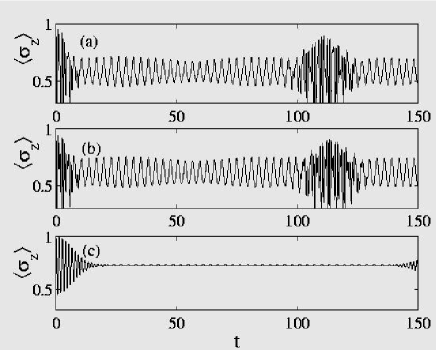
Figure 7: The atomic inversion for the Rabi model (a), adiabatic approximation of the Rabi model (b) and JC model (c). Clearly the JC model does not describe the dynamics properly in this case. The parameters are $\Omega=5$, $g_{0}=0.3$ and $\nu=4$.

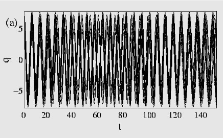
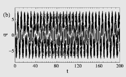
Figure 8: The absolute amplitudes of the wave packets are shown in (a) corresponding to the Rabi case of the previous figure 7, and (b) for the JC model. The two parts first come out of phase (collapse) and then return back in phase (revival). It is seen that the revival occurs at later times with the JC, as seen also in the previous figure.

At some point, the adiabatic approximation breaks down and the above picture of the collapse-revivals fails. Still one may have interesting collapse-revival patters, as is seen in fig. 9. This figure shows the same as fig. 7, but for the parameters $\Omega=0.2$, $\nu=4$ and $g_{0}=2$. The revivals are present in the Rabi model and seem very stable, while in the adiabatic and JC situations they die out fast. The amplitudes of the wave packets are displayed in fig. 10, where (a) gives the Rabi case and (b) the JC situation. The plot clearly indicates the existence of the collapse-revival effect. As the adiabatic approximation is not valid we can no longer try to understand the evolution from the an adiabatic point of view. However, since $\Omega<g_{0}\langle n\rangle$ one may see the wave packet as evolving along the diabatic energies described by the displaced harmonic oscillators. Now they share the same frequency $\omega$ (the anharmonicity comes from the avoided level crossing), so that the oscillation periods are identical. Just like in fig. 5 (a), we see revivals in fig. 9 (a), which occur when the splitted wave packets return to their initial position. For other parameter regimes, where neither the adiabatic nor the diabatic frame holds, the inversion pattern for the Rabi model looks more random.

Figure 9: Same as fig. 7, but with $\Omega=0.2$ and $g_{0}=2$ instead. The revivals are most pronounced for the non-RWA case (a).

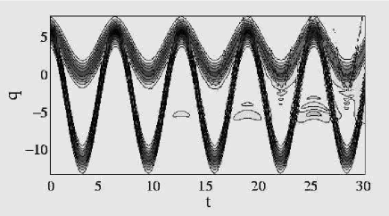
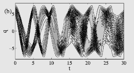
Figure 10: The absolute amplitudes of the original basis ($\{|\pm\rangle\}$) wave packets $\psi_{\pm}(q,t)$ corresponding to the previous fig. 9. Plot (a) gives the amplitudes for the Rabi model and the (b) the same for the JC model.

V.3 Squeezing

Another non-classical property of the field interacting with an atom is squeezing, see jcsqueez . The field is said to be squeezed if one of the quadrature measures $\langle\Delta q^{2}\rangle=\langle q^{2}\rangle-\langle q\rangle^{2}$ or $\langle\Delta p^{2}\rangle=\langle p^{2}\rangle-\langle p\rangle^{2}$ is smaller than 1/2. The Squeezing in the Rabi model has been studied in rabisqueez , and it was found that squeezing for the vacuum is mostly pronounced when $\Omega\gg g_{0}$ and $g_{0}^{2}\gg\Omega$. The second condition implies that the lower adiabatic energy curve has two minima, as in fig. 1 (b)-(d). Dipole squeezing for the Rabi model was considered in disq . In the standard JC model, the amount of squeezing is improved for large amplitude initial states, meaning states with a large average number of photons. The asymptotic solutions in these limits have been applied to study squeezing of the JC model gbsqueez .

In fig. 11 the quadrature for $q$ is shown for four different cases. In the first two plots, (a) and (b), the state of the field is initially in vacuum and (a) $g_{0}=0.1$ and $\Omega=0.2$, while in (b) $g_{0}=0.1$ and $\Omega=2$. In rabisqueez , it is shown that enhanced squeezing may be achieved if the atom is initially in a linear combination of its internal states, such that the wave packet is evolving mainly on one of the adiabatic energy curves. This comes from the fact that squeezing comes from the anharmonicity of the energy curves. Note that in both (a) and (b) the system is highly detuned ($\Omega=2,0.2$) resulting in a small squeezing. In (c) and (d) the state of the field is initially in a coherent state with $\nu=4$, and (c) $g_{0}=0.3$ and $\Omega=5$, and in (d) $g_{0}=0.2$ and $\Omega=1$. Thus, in (d) the system is in resonance, $\Omega=\omega$.

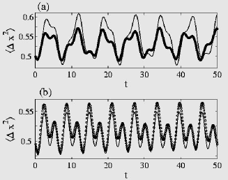
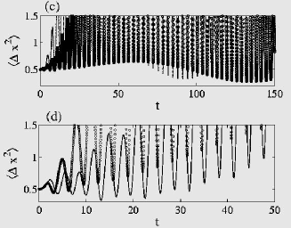
Figure 11: The absolute quadrature $\langle\Delta x^{2}\rangle$ for the JC (circles) and the Rabi (solid) models. In (a) $g_{0}=0.1$, $\Omega=0.2$ and $\nu=0$, in (b) $g_{0}=0.1$, $\Omega=2$ and $\nu=0$, in (c) $g_{0}=0.3$, $\Omega=5$ and $\nu=4$ and in (d) $g_{0}=0.2$, $\Omega=1$ and $\nu=4$.

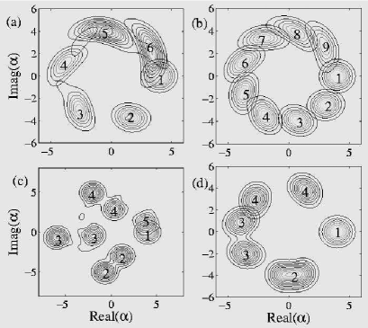
Figure 12: Evolution of the $Q$-function for the Rabi model (left plots) and the JC model (right plots). In (a) and (b) $g_{0}=0.3$, $\Omega=5$ and $\nu=4$, while in (c) and (d) we display a resonant situation $\Omega=1$, and with $g_{0}=1$. Numbers indicate time ordering and the final times (indicated by up to 9 in (a) and (b) and by up to 5 in (c) and (d)) are $t_{f}=400$ for the upper plots and $t_{f}=6$ for the lower ones.

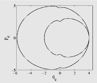
Figure 13: The classically obtained phase space trajectories (41) corresponding to the previous example of fig. 12 (c).

Squeezing also manifests itself in the various quasi phase distributions of the field. Here we give examples of the $Q$-function lamb , defined as $Q(\alpha)=\pi^{-1}\langle\alpha|\rho_{f}|\alpha\rangle$, where $|\alpha\rangle$ is a coherent state, and $\rho_{f}=\langle+|\rho|+\rangle+\langle-|\rho|-\rangle$ is the field density operator and $\rho$ the full atom-field density operator. For a coherent state of the field, the $Q$-function is given by a symmetric Gaussian in the complex $\alpha$-plane, while if it is squeezed, the Gaussian is no longer symmetric, but squeezed in some direction. The $Q$-function for various types of JC models has been studied in jcq and for the Rabi model in rabiq . Figure 12 gives the $Q$-function at different times for the Rabi model (left plots) and for the JC model (right plots), with an initial coherent state with $\nu=4$. In (a) and (b) $g_{0}=0.3$ and $\Omega=5$, and therefor the system is largely detuned which is seen since the $Q$-function does not split into two clear parts, as in (c) and (d) where $g_{0}=1$ and $\Omega=1$. In the last two plots the $Q$-function clearly splits up, however it is seen that for the Rabi model the two parts of the function comes back in phase contrary to what is seen for the JC model. The total time evolved in (a) and (b) is $t_{f}=400$, while in (c) and (d) it is only $t_{f}=6$. Since the coupling is larger in (c) and (d) together with having the resonance condition, the characteristic timescales become much shorter. During the splitting the system quantities collapse and the revival occurs when the parts come back together again. Therefor, in the Rabi model a revival takes place very early, compared to the JC model. It should also be noted that at half the revival time in the Rabi model the field has split into a Schrödinger cat state cat with approximately same phase but different amplitudes, which was discussed by Phoenix rabiq . This is not the case of the JC model, where the splitting is solely in phase and not amplitude.

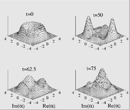
Figure 14: The evolution of a Fock state $|n=6\rangle$ in the Rabi model for different times and $\Omega=1$ and $g_{0}=0.5$.

To understand this amplitude splitting we write $\alpha=\frac{1}{\sqrt{2}}(q_{c}-ip_{c})$ and approximate the real and imaginary parts of $\alpha$ by its classical variables; $\dot{q}_{c}=\frac{\partial H_{\pm}}{\partial p_{c}}$ and $\dot{p}_{c}=-\frac{\partial H_{\pm}}{\partial q_{c}}$. In this semi-classical approximation we use the adiabatic potential (32) as the classical potential governing the evolution $H_{\pm}=\frac{p_{c}^{2}}{2}+V_{\pm}(q_{c})$, and taking into account the level splitting (replace $q_{c}$ by $|q_{c}|$ in the last term), we find

$$\begin{array}[]{l}\dot{q_{c}}=p_{c},\\ \\ \displaystyle{\dot{p_{c}}=-q_{c}+\frac{16\Omega^{2}g_{0}^{4}q_{c}}{\left(\Omega^{2}+2g_{0}^{2}q_{c}^{2}\right)^{3}}\mp\frac{4g_{0}^{2}|q_{c}|}{\sqrt{\Omega^{2}+8g_{0}^{2}q_{c}^{2}}}},\end{array}$$ (41)

where the $\mp$-sign corresponds to which potential sheet $V_{\pm}(q_{c})$ is being used. In fig. 13 we present the classical phase space trajectories for the example of fig. 12 (c). The ’kinks’ at $q_{c}=0$ are due to the second term of $V_{\pm}(q)$ in eq. (32), arising from the variations of the potential. For the JC system, on the other hand, the Hamilton equations of motion are of the form

$$\begin{array}[]{l}\dot{q_{c}}=f_{\pm}(q_{c},p_{c}),\\ \\ \displaystyle{\dot{p_{c}}=-f_{\pm}(p_{c},q_{c})},\end{array}$$ (42)

resulting in perfect circular trajectories due to the rotational symmetry in 2-d. Another way to explain this splitting is given in clsb , where one considers the energy manifolds

$$\varepsilon_{\pm}(p,q)=\frac{p^{2}}{2}+\frac{q^{2}}{2}\pm\sqrt{\frac{\Omega^{2}}{4}+2g_{0}^{2}q^{2}}.$$ (43)

The contours obtained by keeping $\varepsilon_{\pm}(p,q)=\varepsilon_{0}$, where $\varepsilon_{0}$ is the initial energy, govern the adiabatic trajectories in phase space.

As was noted above for the resonant situation and strong coupling, $g_{0}\sim\omega$, the Rabi model gives very interesting behaviours, different from the JC model. This does not only happen for initial coherent field states. For a Fock state $|n\rangle$, the $Q$-function is a ”ring” with radii $|\alpha|=\sqrt{n}$ and thus completely undetermined phase. In the JC model, a Fock state evolves according to Rabi oscillations between $|n\rangle$ and $|n+1\rangle$ (the atom is initially in the excited state $|+\rangle$), and therefor, the $Q$-function will have a ”breathing” amplitude motion, but the phase stays undetermined. For the Rabi model however, the phase may not stay equally distributed over $2\pi$, and sort of cat states may form. This is verified in fig. 14, where the $Q$-function is plotted for four different times, $t=0,50,62.5$ and 75 for an initial Fock state with $n=6$ and $\Omega=1$ and $g_{0}=0.5$. Clearly, at some specific times $t$, the $Q$-function consists of four distinct blobs and at other times two. For other initial Fock states and other parameters one may obtain $Q$-functions consisting of more than four blobs. These states could be of interest for quantum information processing qinfo .

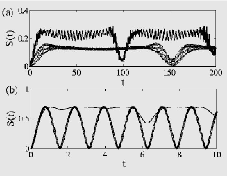
Figure 15: The entropy for an initial coherent state (a) as in fig. 7 but with $\nu=3$, and a Fock state (b) with $g_{0}=1$, $\Omega=1$ and $n=0$. Circles display the entropy for the JC model and solid line the Rabi results.

V.4 Entanglement

Figure 16: The absolute value of the autocorrelation function for the JC (solid line) and the Rabi (dotted line) model, for an initial coherent state with $\nu=15$ and $g_{0}=1$ and $\Omega=1$ (a) and $g_{0}=0.3$ and $\Omega=5$ (b).

The entanglement shared between the field and the atom is well studied in the JC model entangle . For example, it is known that for initial coherent states of the field, the atom is entangled with the field at all times except for half the revival times, where it disentangles from the field provided a large field amplitude gb . Also for the Rabi model, entanglement has been analysed rabient . There are many measures of entanglement between two interacting subsystems $A$ and $B$, where one of the more established ones is the von Neumann entropy

$$S_{A}=-\mathrm{Tr}\left[\rho_{A}\log\left(\rho_{A}\right)\right],$$ (44)

and $\rho_{A}=\mathrm{Tr}_{B}\left[\rho\right]$ is the reduced density operator for subsystem $A$. For a pure disentangled state we have $S_{A}=0$, and it can be shown that if the system starts out in a pure state $S_{A}(t)=S_{B}(t)$ lieb . For the two-level atom-field system studied here, defining the coefficients

$$c_{n}^{\pm}(t)=\int\psi_{n}^{*}(q)\psi_{\pm}(q,t)\,dq,$$ (45)

we find the eigenvalues $\lambda_{\pm}$ of the reduced density matrix for the atom as

$$\begin{array}[]{lll}\lambda_{\pm}&=&\displaystyle{\frac{1}{2}\pm\sqrt{\frac{1}{4}+\left|\sum_{n}c_{n}^{+}(t)c_{n}^{*-}(t)\right|^{2}}}\\ \\ &&\displaystyle{\sqrt{+\sum_{n}\left|c_{n}^{+}(t)\right|^{2}\left(\sum_{n}\left|c_{n}^{+}(t)\right|^{2}-1\right)}}\end{array}$$ (46)

and the entropy

$$S_{A}=-\lambda_{+}\log\left(\lambda_{+}\right)-\lambda_{-}\log\left(\lambda_{-}\right).$$ (47)

Other measures for entanglement between bipartite systems are possible bengtsson .

Examples of the entropy are presented in fig. 15 for an initial coherent state (a), corresponding to the example of fig 7 but with $\nu=3$, and a Fock state (b) at resonance $\Omega=1$ and $g_{0}=1$. As expected, the entanglement is in general larger in the Rabi model. For the coherent states, we see the typical disentanglement at the revival time in both models. For a Fock state we know that in the JC model, the atom disentangle from the field periodically with the Rabi oscillations. This is not the case in the Rabi model, since a set of Fock states of the field will be coupled to the atom and the disentanglement must occur between all field states and the atom simultaneously.

V.5 Autocorrelation function

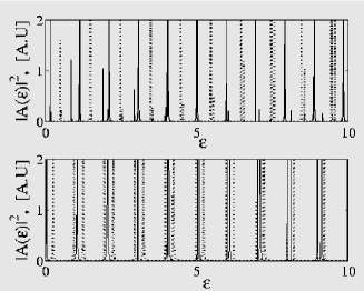
Figure 17: The absolute value squared of the fourier transformed autocorrelation functions of the previous fig. 16. Dotted line corresponds to the Rabi model, while solid line the JC model.

The autocorrelation function

$$A(t,s)=\langle\Psi(t)|\Psi(s)\rangle,\hskip 56.9055ptt>s,$$ (48)

contains much information about the dynamics of a given system. The mathematical properties of the autocorrelation function have been studied by numerous authors auto . Here we will take time $s=0$ (and for simplicity denote the autocorrelation function by $A(t)$), and thus, the autocorrelation function measures fidelity between the initial state and the time evolved state. Expanding the initial state in eigenstates of the Hamiltonian (assuming a discrete spectrum), $|\Psi_{0}\rangle=\sum_{n}c_{n}|\psi_{n}\rangle$, we get

$$A(t)=\sum_{n}\mathrm{e}^{iE_{n}t}|c_{n}|^{2}.$$ (49)

Fourier transforming the autocorrelation function then gives a direct relation to the spectrum, $E_{n}$ of the Hamiltonian

$$|A(\epsilon)|\propto\sum_{n}|c_{n}|^{2}\delta(\epsilon-E_{n}).$$ (50)

Note that in the numerical simulations, time $t$ is given on a lattice and the lattice length $L_{t}$ and spacing $dt$ determine the $\epsilon$-lattice according to the FFT, and also the widths of the $\delta$-function peaks in the spectrum.

In fig. 16 we give an example of the autocorrelation function $A(t)$ for an initial coherent state with amplitude $\nu=15$, and parameters $g_{0}=1$ and $\Omega=1$ (a) and $g_{0}=0.3$ and $\Omega=5$ (b). The dotted line corresponds to the Rabi model while solid line to the JC model. We note that the peaks occur at around times $t=2n\pi$ ($\omega=1$), $n=0,1,2,...$, and that there are two such reviving peaks for each $2n\pi$ and they become more separated for larger times. The autocorrelation function also contains the information about the revival times; when the distance between the two seperated peaks becomes equal to $2\pi$, interference of the wave packets take place resulting in a revival. Since the separation is faster for the JC model in the (a) plot, the revivals will occur earlier in the JC model compared to the Rabi model. The Rabi model seperation is not as smooth as for the JC model which will tend to smear out the revivals, which was already seen in fig. 7. In (b), corresponding to fig. 7, the separation speed is slightly larger for the Rabi model and the revival times is therefor shorter than for the JC model. Measuring the revival times from fig. 16 (a) and (b) for the JC model one finds $t_{R}\approx 94.2$ and $t_{R}\approx 343.4$ respectively, which coincide well with the known analytical approximate expression scully

$$t_{R}\approx 2\pi\frac{\sqrt{\bar{n}}}{g_{0}}\left(1+\frac{\Delta^{2}}{4g_{0}^{2}\bar{n}}\right)^{1/2}.$$ (51)

Since the wave packet evolves on potential surfaces that are not fully harmonic, small spreading occur and the peaks in the autocorrelation function will as well broaden. This in turn leads to decreasing revival amplitudes and the characteristic revival widths become longer, see fig. 9 (c).

Figure 17 shows one part of the fourier transformed autocorrelation functions of fig. 16. Clear peaks indicating the eigen enrgies are noted for both models. There seems to be two different energy spacings between the peaks, one slightly larger and one slightly lower than $\epsilon=1$. In the JC model this is easily understood from the analytic expression (30) for the energies, which for large values on $n$ can be linearly approximated over short $n$-intervals. From the fact that $\bar{n}\gg 1$ it follows that also $q\gg 1$ and we are in the adiabatic regime, where the potential curves are well described by two centered harmonic oscillators with frequencies slightly larger and smaller than one. This, of course, also applies to the Rabi model, and in pertrabi it is shown, in a perturbative way, that the spectrum of the Rabi model approaches an equidistant one in the strong coupling limit. When $\bar{n}$ is decreased the linearization of the energies (30) is no longer justified, which as well follows from the fact that the adiabatic approximation breaks down in such regimes.

VI Conclusions

In this paper we have used a wave packet approach to get a deeper understanding of two of the most commonly used systems in quantum optics and solid state physics; the JC and Rabi models. The wave packet method is purely numerical, but once the evolved wave packets are obtained, all various physical quantities are easily obtainable. Also, for the JC model, which is analytically solvable, one is often left with an infinite sum representing some physical quantity, and either approximations or numerical methods are used to get a ”closed” form of the quantity. More important, from the knowledge of how the wave packet evolves on the two coupled potential curves, one can understand several phenomena such as Rabi oscillations, entanglement and collapse-revivals, and even find approximate results for some quantities in the adiabatic or diabatic limits. Another advantage of this approach is that it is numerically easily obtained for any parameter regimes, especially in the strong coupling regime, where other approaches such as truncation methods tend to be cumbersome.

The focus has been to study some of the known phenomena of the models and compare the two. Several differences have been observed, and, of course, especially when the RWA is known to break down. The comparison between the two models is, however, mainly to understand the wave packet evolutions, and not to point out the physical differences between the two. For very strong couplings, the Rabi model shows many interesting effects, for example splitting of the phase-space function into several parts, and also splitting in amplitude. This effect has not been studied in detail earlier rabiq . Another interesting aspect seen from the wave packet simulations is the effect of the ”momentum” coupling between the two energy curves, present in the JC model. It has been shown that this term bounds the wave packet close to the origin, making it not slide down the two energy curves. The link between the JC model and curve crossing problems is of great interest since knowledge from either of the two may give insight into the other one. The semi-classical treatment presented in subsection II.3 shows how to derive time dependent two-level Hamiltonians, which have aspplications in several fields of quantum mechanics ccross ; ccross2 .

The method of wave packet propagation may easily be applied to similar or extended models, for example Kerr systems kerr , pumped systems pump , the Dicke model lamb ; dickem and multi-level models multilev and it is believed that much insight of these systems may be gained. The relation between the models studied in this paper and models describing diatomic molecular dynamics is planed for a future project (see also molekyl ), and especially study the effect of anharmonicity in the potential curves on the physical quantities. For such analysis it is likely that shape invariant potential techniques (SUSY) may be applicable susy . Interference effects between the evolved wave packets, but for a molecular system, will be presented elsewhere asa . These results may have interesting applications in the JC or Rabi model.

- (1) E. T. Jaynes, and F. W. Cummings, Proc. IEEE 51, 89 (1963).
- (2) B. W. Shore, and P. L. Knight, J. Mod. Opt. 40, 1195 (1993).
- (3) I. I. Rabi, Phys. Rev. 49, 324 (1926); 51, 652 (1937).
- (4) L. Allen and J. H. Eberly, Optical Resonance and Two-level Atoms (Dover Publications, 1087).
- (5) M. D. Crisp, Phys. Rev. A 43, 2430 (1991).
- (6) Quantum entanglement and information processing, edited by D. Esteve, J. -M. Raimond, and J. Dalibard, (Elsevier, 2004).
- (7) J. H. Eberly, N. B. Narozhny, and J. J. Sanchez-Mondragon, Phys. Rev. Lett. 44, 1323 (1980); N. B. Narozhny, J. J. Sanchez-Mondragon, and J. H. Eberly, Phys. Rev. A 23, 236 (1981); G. Rempe, and H. Walther, Phys. Rev. Lett. 58, 353 (1987).
- (8) J. R. Kuklinski, and J. L. Madajczyk, Phys. Rev. A 37, 3175 (1988); M. Hillery, Phys. Rev. A 39, 1556 (1989).
- (9) S. J. D.Phoenix, and P. L. Knight, Phys. Rev. A 44, 6023 (1991); S. Furuichi, and M. Ohya, Lett. Math. Phys. 49, 279 (1999); S. Bose, I. Fuentes-Guridi, P. L. Knight, and V. Vedral, Phys. rev. Lett. 87, 050401 (2001).
- (10) M. Brune, S. Haroche, J. M. Raimond, L. Davidovich, and N. Zagury, Phys. Rev. A 45, 5193 (1992); G. C. Guo, and S. B. Zheng, Phys. Lett. A 223, 332 (1996); C. C. gerry, Phys. Rev. Lett. 55, 2478 (1997); C. C. Gerry, Phys. Rev. B 57, 7474 (1998); S. E. Barnes, Phys. Rev. Lett. 87, 167201 (2001).
- (11) J. J. Slosser, P. Meystre, and S. L. Braunstein, Phys. Rev. Lett. 63, 934 (1989); M. Weidinger, B. T. H. Varcoe, R. Heerlein, and H. Walther, Phys. Rev. Lett. 82, 3795 (1999); S. Brattke, B. T. H. Varcoe, and H. Walther, Phys. Rev. Lett. 86, 3534 (2001).
- (12) H. J. Carmichael, Phys. Rev. Lett. 55, 2790 (1985); P. K. Aravind, J. Opt. Soc. Am. A 4, 26 (1987); M. Hennrich, A. Kuhn, and G. Rempe, Phys. Rev. Lett. 94, 053604 (2005); F. Dubin, D. Rotter, M. Mukherjee, C. Russo, J. Eschner, and R. Blatt, quant-ph/0610065.
- (13) D. Leibfried, R. Blatt, C. Monroe, and D. Wineland, Rev. Mod. Phys. 75, 281 (2003).
- (14) J. M. Raimond, M. Brune, and S. Haroche, Semicond. Sci. Technol. 17, 355 (2002); E. K. Irish, and K. Schwab, Phys. Rev. B 68, 155311 (2003); A. Wallraf, D. I. Schuster, A. Blais, L. Frunzio, J. Majer, M. H. Devoret, S. M. Girvin, and R. J. Schoelkopf, Nature 431, 162 (2004).
- (15) I. Chiorescu, P. Bertet, K. Semba, Y. Nakamura, C. J. P. M. Harmans, and J. E. Mooil, Nature 431, 159 (2004).
- (16) N. Hatakenaka, and S. Kurihara, Phys. Rev. A 54, 1729 (1996); A. T. Sornborger, A. N. Cleland, and M. R. Geller, Phys. Rev. A 70, 052315 (2004);.
- (17) J. M. Raimond, M. Brune, and S. Haroche, Rev. Mod. Phys. 73, 565 (2001).
- (18) D. Meiser, and P. Meystre, quant-ph/0605020.
- (19) A. A. Clerk, and J. E. Sipe, Found. Phys. 28, 639 (1998); I. Dolce, R. Passante, and F. Persico, Phys. Lett. A 155, 152 (2006).
- (20) V. E. Lembessis, and D. Ellinas, J. Opt. B: Quant. Semiclass. 7, 319 (2005).
- (21) G. Berlin, and J. Alinga, J. Opt. B: Quant. Semiclass. 6, 231 (2004).
- (22) S. Guerin, R. G. Unanyan, L. P. Yatsenko, and H. R. Jauslin, Opt. Exress 4, 84 (1999); J. Cheng, and J. Zhon, Phys. Rev. A 64, 065402 (2001).
- (23) V. Kimberg, F. F. Guimaraes, V. C. Felicissimo, and F. Gelmakhanor, Phys. Rev. A 73, 023409 (2006).
- (24) M. A. Kmetic, and W. J. Meath, Phys. Rev A 41, 1556 (1990); A. Brown, W. J. Meath, and P. Tran, Phys. Rev A 65, 063401 (2002).
- (25) F. De Zela, E. Solano, and A. Gago, Opt. Commun. 142, 106 (1997); Z. Liu, and L. Zeng, J. Mod. Opt. 45, 945 (1998); F. De Zela, Lecture Notes in Physics 575, 310 (2001).
- (26) M. Jalenska-Kuklinska, and M. Kus, Phys. Rev. A 41, 2889 (1988); R. Graham, and M. Höhnerbach, Z. Phys. B 57, 233 (1984).
- (27) A. A. Ferro, J. D. Hybil, and D. M. Jones, J. Chem. Phys. 114, 4649 (2001); C. Serrat, arXiv: org:phys/0507061;
- (28) Z. Dutton, K. U. R. M. Murali, W. D. Oliver, and T. P. Orlando, Phys. Rev. B 73, 104516 (2006).
- (29) A. Kujawski, Z. Phys. B 85, 129 (1991).
- (30) J. C. Peploski, and L. Eno, J. Chem. Phys. 88, 6303 (1988).
- (31) M. Kus̀, and M. Lewenstein, J. Phys. A: Math. Gen. 19, 305 (1984); H. G. Reik, M. Doucha, Phys. Rev. Lett. 57, 787 (1986); H. G. Riek, P. Lais, M. E. Stutzle, and M. Doucha, J. Phys. A: Math. Gen. 20, 6327 (1987).
- (32) S. J. D. Phoenix, J. Mod. Opt. 36, 1163 (1989).
- (33) K. Zaheer, and M. S. Zubairy, Opt. Comm. 73, 325 (1989).
- (34) S. J. D. Phoenix, J. Mod. Opt. 38, 695 (1991); G. A. Finney, and J. Gea-Banacloche, Phys. Rev. A 50, 2040 (1994).
- (35) J. S. Peng, and G.-X. Li, Phys. Rev. A 45, 3289 (1992).
- (36) M. F. Fang, and P. Zhou, Physica A 234, 571 (1996).
- (37) E. A. Tur, Opt. Spectro. 91, 899 (2001); E. A. Tur, arXiv: math-ph/0211055.
- (38) K. Zaheer, and M. S. Zubairy, Phys. Rev. A 37, 1628 (1988).
- (39) S. Swain, J. Phys. A: Math. Gen. 6, 192 (1973); S. Swain, J. Phys. A: Math. Gen. 6, 1919 (1973); E. A. Tur, Opt. Spectro. 89, 574 (2000).
- (40) G. Benivegna, and A. Messina, Phys. Rev. A 35, 3313 (1987); G. Qin, K.-L. Wang, T.-Z. Li, R.-S. Han, and M. Feng, Phys. Lett. A 239, 272 (1998); R. F. Bishop, N. J. Davidson, R. M. Quick, and D. M. van der Walt, Phys. Lett. A 254, 215 (1999).
- (41) R. F. Bishop, N. J. Davidson, R. M. Quick, and D. M. va n der Walt, Phys. Rev. A 54, R4657 (1996); R. F. Bishop, and C. Emary, J. Phys. A: Math. Gen. 34, 5635 (2001).
- (42) M. D. Crisp, Phys. Rev. A 46, 4138 (1992).
- (43) E. K. Irish, J. Gea-Banacloche, I. Martin, and K. C. Schwab, Phys. Rev. B 72, 195410 (2005).
- (44) A. Pereverzev, and E. R. Bittner, quant-ph/0510225.
- (45) T. Sandu, arXiv:cond-mat/0608483.
- (46) T. Sandu, V. Chihaia, and W. P. Kirk, J. Lumin. 101, 1001 (1993).
- (47) M. I. Salkola, A. R. Bishop, V. M. Kenkre, and S. Raghavan, Phys. Rev. B 54, R12645 (1996).
- (48) R.-H. Xie, T.-J. Zhou, and Q. Rao, J. Mod. Opt. 43, 337 (1996).
- (49) I. D. Feranchuk, L. I. Komarov, and A. P. Ulyanenkov, J. Phys. A: Math. Gen. 29, 4035 (1996).
- (50) J. Q. Shen, quant-ph/0311140.
- (51) P. W. Milonni, J. R. Ackerhalt, and H. W. Galbraith, Phys. Rev. A 50, 966 (1983); M. Kus, Phys. Rev. Lett. 54, 1343 (1985); A. Kujawski, and M. Munz, Z. Phys. B 76, 273 (1989); L. Mller, J. Stolze, H. Leschke, and P. Nagel, Phys. Rev. A 44, 1343 (1991).
- (52) T. Fukuo, T. Ogawa, and K. Nakamura, Phys. Rev. A 58, 3293 (1998).
- (53) V. Bargmann, Pure Appl. Math. 14, 187 (1961); V. Bargmann, Proc. Natl Acad. Sci. U.S. 48, 199 (1962).
- (54) S. Stenholm, Opt. Commun. 36, 75 (1981).
- (55) S. Schweber. Ann. Phys. 41, 205 (1967); M. Szopa, G. Mys, and A. Ceulemans, J. Phys. A: Math. Gen. 37, 5402 (1996).
- (56) F. T Smith, Phys. Rev. 179, 111 (1969); J. B. Delos, and W. R. Thorson, J. Chem. Phys. 70, 1775 (1979).
- (57) M. Wagner, Z. Phys. B 32, 225 (1979).
- (58) L. D. Landau, Phys. Z. Sowjet Union 2, 46 (1932); C. Zener, Proc. R. Soc. Lond. A 137, 696 (1932).
- (59) M. O. Scully, and M. S. Zubairy, Quantum optics, (Cambridge, 1997).
- (60) J. Larson, J. Salo, and S. Stenholm, Phys. Rev. A 72, 013814 (2005).
- (61) M. Holthaus, J. Opt. B: Quant. Semiclass. Opt. 2, 589 (1999).
- (62) M. S. Child, Molecular Collision Theory, (Dover Publications, New York 1974); B. W. Shore, The Theory of Coherent Atomic Excitation, (John Wiley & Sons, New York 1990); E. E. Nikitin, and S. Ya. Umenskii, The theory of Slow Atomic Collisions, (Springer verlag, Heidelberg 1999).
- (63) Bohm, Quantum Mechanics, (Dover Publications, New York 1989); Messiah, Quantum Mechanics, (Dover Publications, New York 1999).
- (64) S. Teufel, Adiabatic Perturbation Theory in Quantum Dynamics, (Springer, 2003).
- (65) J. Larson, and S. Stenholm, Phys. Rev. A 73, 033805 (2006). (2006).
- (66) M. Alexanian, and S. K. Bose, Phys. Rev. A 52, 2218 (1995); A. B. Klimov, and L. L. Sanchez-Soto, Phys. Rev. A 61, 063802 (2000); A. B. Klimov, L. L. Sanchez-Soto, A. Navarro, and E. C. Yustas, J. Mod. Opt. 49, 2211 (2002).
- (67) M. D. Fleit, J. A. Fleck, and A. Steiger, J. Comp. Phys. 47, 412 (1982).
- (68) M. Frasca, Phys. Rev. A 66, 023810 (2002); K. Fujii, J. Phys. A: Math. Gen. 36, 2109 (2003).
- (69) R. W. Robinett, Phys. Rep. 392, 1 (2004).
- (70) M. V. Satyanarayana, P. Rice, R. Vyas, and H. J. Carmichel, J. Opt. Soc. Am. B 6, 228 (1989); S. S. Averbukh, Phys. Rev. A 46, R2205 (1992); P. F. Góra, and C. Jedrzejek, Phys. Rev. A 48, 3291 (1993).
- (71) C. W. Woods, and J. Gea-Banacloche, J. Mod. Opt 40, 2361 (1993).
- (72) L. Mandel, and E. Wolf, Optical Coherence and Quantum Optics, (Cambridge, 1995).
- (73) M. J. Werner, and H. Risken, Quant. Opt. 3, 185 (1991); J. Eiselt, and H. Risken, Phys. Rev. A 43, 346 (1991); C. A. Miller, J. Hilsenbeck, and H. Risken, Phys. Rev. A 46, 4323 (1992).
- (74) M. A. Nielsem, and I. l. Chuang, Quantum Computing and Quantum information, (Cambridge, 2000); H. Jeong, and T. C. Ralph, quant-ph/0509137.
- (75) J. Gea-Banacloche, Phys. Rev. Lett. 65, 3385 (1990); J. Gea-Banachloche, Phys. Rev. A 44, 5913 (1991); V. Buzek, H. Moya-Cessa, P. L. KNight, and S. J. D. Phoenix, Phys. Rev. A 45, 8190 (1992); A. Auffeves, P. Maioli, T. Meunier, S. Gleyzes, G. Nogues, M. Brune, J. M. Raimond, and S. Haroche, Phys. Rev. Lett 91, 230405 (2003).
- (76) H. Araki, and E. Lieb, Comm. Math. Phys. 18, 160 (1970).
- (77) I. Bengtsson, and K. Ẑyczkowski, Geometry of Quantum States, (Cambridge University Press, 2006).
- (78) H. Bohr, Almost periodic functions, (Chelsea, New York 1947); P. Bocchieri, and A. Loinger, Phys. Rev. 107, 337 (1957); R. von Baltz, Eur. J. Phys. 11, 215 (1990).
- (79) N. Rosen, and C. Zener, Phys. Rev. 40, 502 (1932); Y. N. Demkov, and M. Kunike, Vestn. Leningr. Univ. Ser. Fiz. Khim. 16, 39 (1969); A. Bambini, and P. R. Berman, Phys. Rev. A 23, 2496 (1981); F. T. Hioe, and C. E. Carroll, J. Opt. Soc Am. B 2, 497 (1985); B. M. Garraway, and K. -A. Suominen, Rep. Prog. Phys. 58, 365 (1995)
- (80) G. S. Agarwal, and R. R. Puri, Phys. Rev. A 39, 2 969 (1989); A. Joshi, and R. R. Puri, Phys. Rev. A 45, 5056 (1992); J. Liu, and Y. Wang, Phys. Rev. A 54, 2326 (1996).
- (81) P. Alsing, D. S. Guo, and H. J. Carmichael, Phys. Rev. A 45, 5135 (1992); C. C. Gerry, Phys. Rev. A 65, 063801 (2002); E. Solano, G. S. Agarwal, and H. Walther, Phys. Rev. Lett. 90, 027903 (2003); H. Moya-Cessa, D. Jonathan, and P. L. Knight, J. Mod. Opt. 50, 265 (2003); J. Gea-Banacloche, T. C. Rice, and L. A. Orozco, Phys. Rev. Lett. 94, 053603 (2005).
- (82) Y. K. Wang, and F. T. Hioe, Phys. Rev. A 7, 831 (1973); M. Frasca, J. Phys. B: At. Mol. Opt. Phys. 37, 1273 (2004); W. Hou, and B. B. Hu, Phys. Rev. A 69, 042110 (2004).
- (83) A. Messina, S. Maniscalco, and A. Napoli, J. Mod. Opt. 50, 1 (2003).
- (84) R. D. Coalson, J. Chem. Phys. 86, 995 (1987); J. Alvarellos, and H. Metiu, J. Chem. Phys. 88, 4957 (1988); A. Eisfeld, L. Braun, W. T. Strunz, J. S. Briggs, J. Beck, and V. Engel, J. Chem. Phys. 122, 134103 (2005).
- (85) A. N. F. Aleixo, A. B. Balantekin, and M. A. C. Ribeiro, J. Phys. A: Math. Gen. 33, 3173 (2000);A. N. F. Alexio, and A. B. Balantekin, J. Phys. A: Math. Gen. 38, 8603 (2005).
- (86) W. Dong, Å. Larson, and T. Hansson, in preparation.