Information/disturbance trade-off in single and sequential measurements on a qudit signal

Abstract

We address the trade-off between information gain and state disturbance in measurement performed on qudit systems and devise a class of optimal measurement schemes that saturate the ultimate bound imposed by quantum mechanics to estimation and transmission fidelities. The schemes are minimal, i.e. they involve a single additional probe qudit, and optimal, i.e. they provide the maximum amount of information compatible with a given level of disturbance. The performances of optimal single-user schemes in extracting information by sequential measurements in a $N$-user transmission line are also investigated, and the optimality is analyzed by explicit evaluation of fidelities. We found that the estimation fidelity does not depend on the number of users, neither for single-measure inference nor for collective one, whereas the transmission fidelity decreases with $N$. The resulting trade-off is no longer optimal and degrades with increasing $N$. We found that optimality can be restored by an effective preparation of the probe states and present explicitly calculations for the 2-user case.

1 Introduction

Any measurement aimed to extract information about a quantum state alters the state itself, i.e. introduces a disturbance [1]. In addition, quantum information cannot be perfectly copied, neither locally [2] nor at distance [3]. Overall, there is an information/disturbance trade-off which unavoidably limits the accuracy of any kind of measurement, independently of the implementation scheme [4]. On the other hand, in a multiuser transmission line each user should decode the transmitted symbol and leave the carrier for the subsequent user. Indeed, what they need is a device able to retrieve as much information as possible, without destroying the carrier. Since in a quantum channel symbols are necessarily encoded in states of a physical system, the ultimate bounds on the channel performances are posed by quantum mechanics.

The trade-off between information gain and quantum state disturbance can be quantified using fidelities. Let us describe a generic scheme for indirect measurement as a quantum operation, i.e. without referring to any explicit unitary realization. The operation is described by a set of measurement operators $\{A_{k}\}$, with the trace-preserving condition $\sum_{k}A^{\dagger}_{k}A_{k}={\mathbbm{I}}$. The probability-operator measure (POVM) of the measurement is given by $\{\Pi_{k}\equiv A_{k}^{\dagger}A_{k}\}$, whereas its action on the input state is expressed as $\varrho\rightarrow\sum_{k}A_{k}\varrho A_{k}^{\dagger}$. This means that, if $\varrho$ is the initial quantum state of the system under investigation, the probability distribution of the outcomes is given by $p_{k}=\hbox{Tr}[\varrho\>\Pi_{k}]=\hbox{Tr}[\varrho\>A^{\dagger}_{k}A_{k}]$. The conditional output state, after having detected the outcome $k$, is given by $\sigma_{k}=\>A_{k}\varrho A_{k}^{\dagger}/p_{k}$, whereas the overall quantum state after the measurement is described by the density matrix $\sigma=\sum_{k}p_{k}\>\sigma_{k}=\sum_{k}A_{k}\varrho A_{k}^{\dagger}$.

Suppose you have a quantum system prepared in a pure state $|\psi\rangle$. If the outcome $k$ is observed at the output of the measuring device, then the estimated signal state is given by $|\phi_{k}\rangle$ (the typical inference rule being $k\rightarrow|\phi_{k}\rangle$ with $|\phi_{k}\rangle$ given by the set of eigenstates of the measured observable), whereas the conditional state $|\psi_{k}\rangle=1/\sqrt{p_{k}}A_{k}|\psi\rangle$ is left for the subsequent user. The amount of disturbance is quantified by evaluating the overlap of the conditional state $|\psi_{k}\rangle$ to the initial one $|\psi\rangle$, whereas the amount of information extracted by the measurement corresponds to the overlap of the inferred state $|\phi_{k}\rangle$ to the initial one. The corresponding fidelities, for a given input signal $|\psi\rangle$, are given by

$$F_{\psi} =\sum_{k}p_{k}\frac{|\langle\psi|A_{k}|\psi\rangle|^{2}}{p_{k}}=\sum_{k}|\langle\psi|A_{k}|\psi\rangle|^{2}$$ (1)

$$G_{\psi} =\sum_{k}p_{k}|\langle\psi|\phi_{k}\rangle|^{2}\;,$$ (2)

where we have already performed the average over the outcomes. The relevant quantities to assess the performances of the device are given by the average fidelities

$$F=\int_{\mathbbm{A}}d\psi\>F_{\psi}\qquad G=\int_{\mathbbm{A}}d\psi\>G_{\psi}\;,$$ (3)

which are obtained by averaging $F_{\psi}$ and $G_{\psi}$ over the possible input states, i.e. over the alphabet ${\mathbbm{A}}$ of transmittable symbols (states). $F$ will be referred to as the transmission fidelity and $G$ to as the estimation fidelity.

Let us first consider two extreme cases. If nothing is done, the signal is preserved and thus $F=1$. However, at the same time, our estimation has to be random and thus $G=1/d$ where $d$ is the dimension of the Hilbert space. This corresponds to a blind quantum repeater [13] which re-prepares any quantum state received at the input, without gaining any information on it. The opposite case is when the maximum information is gained on the signal, i.e. when the optimal estimation strategy for a single copy is adopted [14, 15, 16]. In this case $G=2/(d+1)$, but then the signal after this operation cannot provide any more information on the initial state and thus $F=2/(d+1)$. In between these two extrema there are intermediate cases, i.e. quantum measurements providing only partial information while partially preserving the quantum state of the signal for subsequent users.

The fidelities $F$ and $G$ are not independent on each other. Assuming that ${\mathbbm{A}}$ corresponds to the set of all possible quantum states, Banaszek [4] has explicitly evaluated the expressions of fidelities in terms of the measurement operators, thus rewriting Eqs. (3) as

$$F =\frac{1}{d(d+1)}\left(d+\sum_{k}\left|\hbox{Tr}\left[A_{k}\right]\right|^{2}\right)\>,$$ (4)

$$G =\frac{1}{d(d+1)}\left(d+\sum_{k}\langle\phi_{k}|\Pi_{k}|\phi_{k}\rangle\right)\;,$$ (5)

where $|\phi_{k}\rangle$ is the set of states used to estimate the initial signal. Of course, the estimation fidelity is maximized upon choosing $|\phi_{k}\rangle$ as the eigenvector of the POVM-element $\Pi_{k}$ corresponding to the maximum eigenvalues.

Using Eqs. (4) and (5)it is possible to derive the ultimate bound that fidelities should satisfy according to quantum mechanics. For randomly distributed $d$-dimensional signals, i.e. when the alphabet ${\mathbbm{A}}$ corresponds to the set of all quantum states of a qudit, the information-disturbance trade-off reads as follows [4]

$$(F-F_{0})^{2}+d^{2}(G-G_{0})^{2}+2(d-2)(F-F_{0})(G-G_{0})\leq\frac{d-1}{(d+1)^{2}}\;,$$ (6)

where $F_{0}=\frac{1}{2}(d+2)/(d+1)$ and $G_{0}=\frac{1}{2}\>3/(d+1)$. From Eq. (6) one may derive the maximum transmission fidelity compatible with a given value of the estimation fidelity or, in other words, the minimum unavoidable amount of noise that is added, in average, to a set of random qudits if one wants to acquire a given amount of information. Notice that the trade-off crucially depends on the alphabet of transmittable symbols. Ultimate bound on fidelities have been derived for different set of signals. These include many copies of identically prepared pure qubits [5], a single copy of a pure state generated by independent phase-shifts [6], an unknown spin coherent state [7], and single copy of an unknown maximally entangled state [8]. Optimal measurement schemes, which saturate the bounds, have been also devised [9, 10, 11] and implemented [12].

In this paper we review our results [9] on the unitary realizations of optimal estimation of qudits and present novel results about the information/disturbance trade-off in a multiuser transmission line. As we will see, our schemes are minimal, since they involve a single additional probe qudit, and optimal i.e. the corresponding fidelities saturate the bound (6). We investigate their performances in extracting information in a multiuser transmission line where the unknown signal state $|\psi\rangle$ is measured sequentially by $N$ users, each of them using optimal single-user device.

The paper is structured as follows. In Section 2 the optimal scheme for the estimation of a generic qudit is reviewed in details. In Section 3 we analyze the trade-off for a multiuser transmission line, focusing attention on low-dimensional qudit ($d=\{2,3,4\}$). The optimal trade-off for qubit in a $2$-user transmission line is explicitly evaluated. Section 4 closes the paper with some concluding remarks.

2 Minimal implementation of optimal measurement schemes for qudit

In this section we describe a class of measurement schemes devised to estimate the state of a random qudit without its destruction [9]. The schemes are minimal, since they involve a single additional probe qudit, and optimal because they saturate the bound (6). The measurement scheme is shown in Fig. 1. The signal qudit is coupled with a probe qudit prepared in the state

$$|\omega\rangle_{p}=\cos\theta|0\rangle_{p}+\gamma\sin\theta\>\frac{1}{\sqrt{d}}\sum_{s=0}^{d-1}|s\rangle_{p}$$ (7)

where $\gamma=\left(\sqrt{1+d\tan^{2}\theta}-1\right)/\sqrt{d}\tan\theta$ is a normalization factor. The interaction is given by the unitary gate ${\mathbf{C}}_{d}$ that acts as ${\mathbf{C}}_{d}|i\rangle|s\rangle_{p}=|i\rangle|i\oplus s\rangle_{p}$ where $\oplus$ denotes sum modulo $d$ [17]. After the interaction the spin of the probe is measured in the $z$-direction.

Figure 1: Minimal implementation of optimal measurement scheme for qudits.

The measurement operators are $A_{k}={}_{p}\langle k|{\mathbf{C}}_{d}|\omega\rangle_{p}=\sum_{ij}(A_{k})_{ij}|i\rangle\langle j|$ where

$$(A_{k})_{ij}=\delta_{ij}\left[\delta_{kj}\cos\theta+\frac{\gamma}{\sqrt{d}}\sin\theta\right]\;.$$ (8)

The inference rule is $k\rightarrow|k\rangle$, where $|k\rangle$ is an eigenstate of $S_{z}$. The fidelities are evaluated using Eqs. (4), (5) and (8), arriving at

$$F = \frac{1}{d+1}\left[1+\left(\cos\theta+\gamma\sqrt{d}\sin\theta\right)^{2}\right]\;,$$ (9)

$$G = \frac{1}{d+1}\left[1+\left(\cos\theta+\frac{\gamma}{\sqrt{d}}\sin\theta\right)^{2}\right]\;.$$ (10)

Upon inserting Eqs. (9) and (10) into Eq. (6) we found that the bound is saturated. In other words, the scheme of Fig. 1 provides an optimal measurement scheme for qudits.

The optimal preparation of the probe state can be intuitively understood as follows: for $\theta=0$ the elements of the measurement operators reduce to $(A_{k})_{ij}=\delta_{ij}\delta_{kj}$, which lead to fidelities $F=2/(d+1)$ and $G=2/(d+1)$, i.e. to the extreme case with the maximum information and maximum noise. On the other hand, for $\theta=\pi/2$ the measurement operator have elements $(A_{k})_{ij}=\delta_{ij}\frac{1}{\sqrt{d}}\sum_{s}\delta_{k,j\oplus s}$ which lead to $F=1$ and $G=1/d$, i.e. to the extreme case where the signal is preserved but the estimation has to be random. In fact, the linear combinations (7) are enough, by varying the value of $\theta$, to explore the entire optimal trade-off (6).

3 Sequential measurements in a multiuser transmission line

Let us consider the multiuser transmission line schematically depicted in Fig. 2. Each of the $N$ users detects the received signal by means of the device described in the previous section. At first we consider all the N probes prepared in the same state (i.e. with the same value of $\theta$). The measurements are sequential, i.e the $k$-th user measures the signal outgoing the $(k-1)$-th measurement stage. If the initial state is $|\psi\rangle$ the first user obtains the result $k_{1}$ with probability $p_{k_{1}}=\langle\psi|A^{\dagger}_{k_{1}}A_{k_{1}}|\psi\rangle$, leaving the conditional state $|\psi_{k_{1}}\rangle=1/\sqrt{p_{k_{1}}}A_{k_{1}}|\psi\rangle$ to the subsequent user. The second user obtains the result $k_{2}$ with conditional probability $p_{k_{2},k_{1}}=\langle\psi|\left(A_{k_{2}}A_{k_{1}}\right)^{\dagger}A_{k_{2}}A_{k_{1}}|\psi\rangle$ and leave the conditional state $|\psi_{k_{1},k_{2}}\rangle=\frac{1}{\sqrt{p_{k_{2}k_{1}}}}A_{k_{2}}A_{k_{1}}|\psi\rangle$. Analogously, the $N$-th user obtains the result $k_{N}$ with conditional probability

$$p_{k_{N},k_{N-1},\dots,k_{1}}=\langle\psi|(A_{k_{N}}A_{k_{N-1}}\dots A_{k_{1}})^{{\dagger}}A_{k_{N}}A_{k_{N-1}}\dots A_{k_{1}}|\psi\rangle\>,$$ (11)

corresponding to the conditional state

$$|\psi_{k_{N},k_{N-1},\dots,k_{1}}\rangle =\frac{A_{k_{N}}A_{k_{N-1}}\dots A_{k_{1}}|\psi\rangle}{\sqrt{p_{k_{N},k_{N-1},\dots,k_{1}}}}\>.$$ (12)

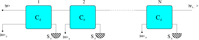
Figure 2: Sequential measurements in a multiuser transmission line.

The unconditional probability of getting the outcome $k$ for the $N$-th user is obtained upon summing over all possible results obtained in the previous $N-1$ steps, i.e.

$$p_{k} =\hbox{Tr}\left[A_{k}\left(\sum_{k_{1},k_{2},\dots,k_{N-1}}A_{k_{N-1}}A_{k_{N-2}}\dots A_{k_{1}}|\psi\rangle\langle\psi|(A_{k_{N-1}}A_{k_{N-2}}\dots A_{k_{1}})^{{\dagger}}\right)A_{k}^{{\dagger}}\right]\>.$$ (13)

The corresponding conditional state reads as follows

$$\varrho_{k}^{N} =\frac{1}{p_{k}}A_{k}\left(\sum_{k_{1},k_{2},\dots,k_{N-1}}A_{k_{N-1}}A_{k_{N-2}}\dots A_{k_{1}}|\psi\rangle\langle\psi|(A_{k_{N-1}}A_{k_{N-2}}\dots A_{k_{1}})^{{\dagger}}\right)A_{k}^{{\dagger}}\>.$$ (14)

Notice that by using the independence of the measurement steps, i.e $\left[A_{k_{i}},A_{k_{j}}\right]=0$, and the normalization condition $\sum_{k_{i}}A_{k_{i}}^{{\dagger}}A_{k_{i}}={\mathbbm{I}}$, $\forall i$, the unconditional probability can be written as $p_{k}=\hbox{Tr}[|\psi\rangle\langle\psi|\>A_{k}^{{\dagger}}A_{k}]$, that is, $p_{k}$ does not depend on the number $N$ of measurement steps. The above formula also indicates that the POVM describing the measurement of the $N$-th user is given by $\{\Pi_{k}=A_{k}^{{\dagger}}A_{k}\}$, which is the same POVM of the single-user scheme described in the previous section. Using the single-measure inference rule $k\rightarrow|k\rangle$, with $|k\rangle$ eigenstate of $S_{z}$, the estimation fidelity $G$ does not depend on the number of measurement steps, and is equal to the single-user one of Eq. (10).

The transmission fidelity at the $N$-th step for a given input signal $|\psi\rangle$ is given by

$$F_{\psi,N} =\sum_{k}p_{k}\hbox{Tr}[|\psi\rangle\langle\psi|\varrho_{k}^{N}]=\sum_{k,k_{1},k_{2},\dots,k_{N-1}}|\langle\psi|A_{k}A_{k_{N-1}}A_{k_{N-2}}\dots A_{k_{1}}|\psi\rangle|^{2}=\sum_{\{k_{i}\}}|\langle\psi|A_{\{k_{i}\}}|\psi\rangle|^{2}$$

where $A_{\{k_{i}\}}=A_{k}A_{k_{N-1}}A_{k_{N-2}}\dots A_{k_{1}}$ and $\sum_{\{k_{i}\}}=\sum_{k}\sum_{k_{N-1}}\sum_{k_{N-2}}\dots\sum_{k_{1}}$ denotes sum over all indices $k_{i}$. Since $\sum_{\{k_{i}\}}A_{\{k_{i}\}}^{{\dagger}}A_{\{k_{i}\}}={\mathbbm{I}}$, we can evaluate the average fidelity by means of (4) with the substitution $k\rightarrow\{k_{i}\}$. Since all the operators commute, the sum can be evaluated as follows

$$\sum_{\{k_{i}\}}\left|\hbox{Tr}\left[A_{\{k_{i}\}}\right]\right|^{2} =\sum_{n_{0}}^{N}\sum_{n_{1}}^{N-n_{0}}\dots\sum_{n_{d-2}}^{N-(n_{0}+\dots+n_{d-3})}\frac{N!}{n_{0}!n_{1}!\dots n_{d-2}!(N-(n_{0}+n_{1}+\dots n_{d-2}))!}$$

$$\times\left|\hbox{Tr}\left[A_{0}^{n_{0}}A_{1}^{n_{1}}\dots A_{d-2}^{n_{d-2}}A_{d-1}^{N-(n_{0}+\dots+n_{d-2})}\right]\right|^{2}$$

where the matrix elements of the operator under trace are given by

$$\left(A_{0}^{n_{0}}A_{1}^{n_{1}}\dots A_{d-2}^{n_{d-2}}A_{d-1}^{N-(n_{0}+\dots+n_{d-2})}\right)_{ij}=\delta_{ij}J(\theta)^{N-n_{i}}L(\theta)^{n_{i}}$$ (15)

with $L(\theta)=\left[(\gamma\sin\theta)/\sqrt{d}+\cos\theta\right]$, $J(\theta)=\left[(\gamma\sin\theta)/\sqrt{d}\right]$ and $n_{d-1}=N-(n_{0}+\dots+n_{d-2})$. For qubit ($d=2$) and qutrit ($d=3$) we obtain

$$F_{N}(d=2) =\frac{1}{3}\left[2+\sin^{2N}\theta\right]\qquad F_{N}(d=3)=\frac{1}{2}\left[1+\sin^{2N}\theta\right]\>.$$ (16)

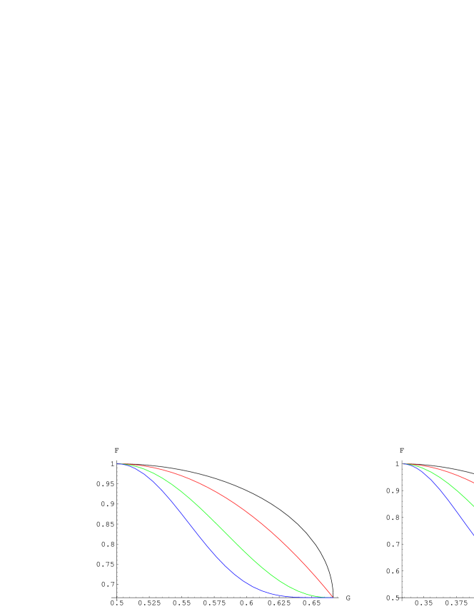
Figure 3: Information/disturbance trade-off for qudit in a $N$-users transmission line. (Black): $N=1$; (Red): $N=2$; (Green): $N=5$; (Blue): $N=10$. From left to right the trade-off for $d=\{2,3,4\}$.

The corresponding information/disturbance trade-offs $F_{N}=F_{N}(G)$ for dimension $d=\{2,3,4\}$ are depicted in Fig. 3 for different values of $N$. As it is apparent from the plots, the trade-off degrades with the number of users $N$.

Let us now consider a different estimation strategy for the scheme depicted in Fig. 2: where the $N$-th user has at disposal the whole set of outcomes $\{k_{i}\}=\{k_{1},k_{2},\dots,k_{N}\}$. The dynamics of the scheme is described by the overall measurement operators $A_{\{k_{i}\}}$. The transmission fidelity does not change whereas the estimation fidelity should be evaluated taking into account the global information coming from the whole set of outcomes. The collective inference rule is given by $\{k_{i}\}\rightarrow\varrho_{\{k_{i}\}}$ where

$$\varrho_{\{k_{i}\}}=\frac{n_{0}}{N}|0\rangle\langle 0|+\frac{n_{1}}{N}|1\rangle\langle 1|+\dots+\frac{N-(n_{0}+n_{1}+\dots+n_{d-2})}{N}|d-1\rangle\langle d-1|$$ (17)

and $n_{j}$ is the number of outcomes $j=\{0,1,\dots,d-1\}$ occurring in the sequence ${\{k_{i}\}}$. The explicit evaluation of the estimation fidelity according to this rule gives the same results of Eq. (10) for dimensions $d=\{2,3,4\}$ (we have been not not able to prove this for any value of $d$). In turn, this means that the trade-off is not altered and shows that taking account collectively the whole set of outcomes does not lead to better performances.

As it is apparent from Fig. 3 there is a region in the $(G,F)$ plane between the optimal trade-off ($N=1$) and the curve corresponding to $N=2$. A question arises on whether the $N=2$ scheme may be optimized in order to reach points in this region. The answer is affirmative, by using a suitable preparation of the probe qudits. In the following we explicitly show how the optimization procedure works in the case of qubit.

Consider two users $A$ and $B$ which prepare their probes with different parameter $\theta_{A}$ and $\theta_{B}$ and then perform a sequential measurement using each the optimal scheme of the previous section. After the second step, the estimation fidelity $G$ is again the optimal one given by Eq. (10) and depends only on the parameter $\theta_{B}$. On the other hand, the transmission fidelity can be calculated by means of (4): the measurement operators $A_{\{k_{i}\}}=A_{k_{B}}A_{k_{A}}$ are given by

$$A_{0}A_{0} =\left(\begin{array}[]{cc}L(\theta_{A})L(\theta_{B})&0\\ 0&J(\theta_{A})J(\theta_{B})\end{array}\right)\qquad A_{0}A_{1}=\left(\begin{array}[]{cc}L(\theta_{B})J(\theta_{A})&0\\ 0&L(\theta_{A})J(\theta_{B})\end{array}\right)$$ (22)

$$A_{1}A_{0} =\left(\begin{array}[]{cc}L(\theta_{A})J(\theta_{B})&0\\ 0&L(\theta_{B})J(\theta_{A})\end{array}\right)\qquad A_{1}A_{1}=\left(\begin{array}[]{cc}J(\theta_{A})J(\theta_{B})&0\\ 0&L(\theta_{A})L(\theta_{B})\end{array}\right)$$ (27)

The fidelity is given by

$$F_{2}(\theta_{A},\theta_{B}) =\frac{1}{24}\left[18-2\cos(2\theta_{A})-2\cos(2\theta_{B})+\cos(2(\theta_{A}-\theta_{B}))+\cos(2(\theta_{A}-\theta_{B}))\right]\>.$$ (28)

The corresponding trade-off is shown in Fig. 4. As a matter of fact, the second user can tune the probe parameter $\theta_{B}$ to achieve points between the optimal trade-off and the curve obtained for $\theta_{A}=\theta_{B}$. In particular, if $\theta_{A}=\pi/2$, i.e. if the first scheme is a blind repeater, then the optimal trade-off can be re-obtained by varying $\theta_{B}$. In the general case, the estimation fidelity can take all the allowed values, while the transmission fidelity $F_{2}$ take values in the range from $F_{min}=2/3$ to $F_{2}(\theta_{A},\pi/2)=(5-\cos 2\theta_{A})/6$. In other words, the user $B$, by knowing the preparation of the first probe and varying the value of $\theta_{B}$, may achieve the desired point on the curves $F=F_{2,\theta_{A}}(G)$ depicted in Fig. 4, i.e. he can tune the trade-off and decide whether improving the estimation fidelity or the transmission fidelity. Besides, this also means that by a suitable choice of both parameters $\theta_{A}$ and $\theta_{B}$, the entire region below the optimal trade-off (bound included) is accessible. The same argument may be applied to $d$-dimensional signals.

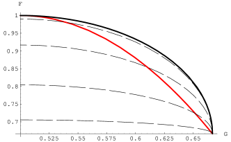
Figure 4: Information/disturbance trade-off for qubits in a $2$-user line with different probes’ parameter $\theta_{A}$ and $\theta_{B}$. In red the trade-off obtained for $\theta_{B}=\theta_{A}$ and varying this single parameter. The black solid line corresponds to the optimal trade-off obtained for $\theta_{A}=\pi/2$ and varying $\theta_{B}$. Black dashed curves correspond to trade-offs $F=F_{2,\theta_{A}}(G)$ obtained varying $\theta_{B}$ at fixed values of $\theta_{A}$. From top to bottom $\theta_{A}=\{4\pi/9;\pi/3;2\pi/9;\pi/9\}$.

4 Conclusions

We have suggested a class of indirect measurement schemes, involving unitary interactions of a signal qudit with a single probe qudit, which are suited to extract information from a random set of qudit signals introducing the minimum amount of disturbance. The schemes are indeed optimal, i.e correspond to estimation and transmission fidelities which saturate the ultimate bound imposed by quantum mechanics. The performances of optimal single-user schemes in extracting information by sequential measurements in a multiuser transmission line have been also investigated. We have explicitly evaluated fidelities and found that estimation fidelity does not depend on the number of users, neither for single-measure inference nor for collective one, whereas the transmission fidelity decreases with the number of steps. The resulting trade-off is no longer optimal and degrades with increasing $N$. Optimality can be restored by a suitable preparation of the probe states: the optimization procedure have been explicitly reported for qubit 2-user case.

This work has been supported by MIUR through the project PRIN-2005024254-002.

References

References

• [1] Hofmann H F, Phys. Rev. A 62, 022103 (2000).
• [2] Wootters W K and Zurek W K, Nature (London) 299, 802 (1982); Buzek V, Hillery M, Phys. Rev. A 54, 1844 (1996); Gisin N, Massar S, Phys. Rev. Lett. 79, 2153 (1997); Werner R F, Phys. Rev. A 58, 1827 (1998).
• [3] Murao M et al., Phys. Rev. A 59, 156 (1999); van Loock P, Braunstein S, Phys Rev Lett. 87, 247901 (2001); Ferraro A et al., J. Opt. Soc. Am. B 21, 1241 (2004).
• [4] Banaszek K, Phys. Rev. Lett. 86, 1366 (2001).
• [5] Banaszek K, Devetak I, Phys. Rev. A 64, 052307 (2001).
• [6] Mista L Jr., Fiurasek J, Filip R. Phys. Rev. A 72, 012311 (2005).
• [7] Sacchi M F , preprint ArXiv quant-ph/0610246.
• [8] Sacchi M F, Phys. Rev. Lett. 96, 220502 (2006).
• [9] Genoni M G , Paris M G A, Phys. Rev. A 71, 052307 (2005).
• [10] Mista L Jr., Filip R, Phys. Rev. A 72, 034307 (2005).
• [11] Buscemi F, Sacchi M F, preprint ArXiV quant-ph/0610232.
• [12] Sciarrino F et al, Phys. Rev. Lett. 96, 020408 (2006).
• [13] Paris M G A, Fortschr. Phys. 51, 202 (2003).
• [14] Massar S and Popescu S, Phys. Rev. Lett. 74, 1259 (1995).
• [15] AcΓ­n A, Latorre J I, Pascual P, Phys. Rev. A 61, 022113 (2000).
• [16] Bruss D and Macchiavello C, Phys. Lett. A 253, 149 (1999).
• [17] Gernot A, Delgado A, Gisin N, Jex I, J. Phys. A 34, 8821