Relation between phase space coverage and entanglement for spin-1/2 systems

Abstract

For systems of two and three spins 1/2 it is known that the second moment of the Husimi function can be related to entanglement properties of the corresponding states. Here, we generalize this relation to an arbitrary number of spins in a pure state. It is shown that the second moment of the Husimi function can be expressed in terms of the lengths of the concurrence vectors for all possible partitions of the $N$-spin system in two subsystems. This relation implies that the phase space distribution of an entangled state is less localized than that of a non-entangled state. As an example, the second moment of the Husimi function is analyzed for an Ising chain subject to a magnetic field perpendicular to the chain axis.

I Introduction

In the last few years there has been growing activity in the study of the behavior of spin chains viewed from a quantum information perspective. The relations between condensed matter physics and quantum information are twofold in this case. On the one hand, spin chains can provide a tool for quantum communication bose03 ; burga05 . On the other hand, the concept of entanglement has been employed to study spin systems, in particular at a quantum phase transition oster02 ; osbor02 ; vidal03 ; lator04 . Furthermore, the concept of matrix product states has led to new insights into the density matrix renormalization group algorithm (DMRG) with which the ground state properties of spin systems can be determined verst04 ; schol05 .

Recently, A. Sugita sugit03 has pointed out for two spins 1/2 a relation between an entanglement measure, the so-called concurrence woott01 , and a property of the phase-space representation of the state of the two spins. More specifically, this relation involves the second moment of the Husimi function, a positive definite phase space distribution. husim40 ; lee95 This quantity can be viewed as an inverse participation ratio in phase space and measures to which extent the phase space is covered by the Husimi function. It turns out that the more the state extends over phase space, the more the state is entangled. In particular, the Husimi function of a factorizable state minimally covers the phase space. A first impression of this difference between the phase space representations of entangled and non-entangled states can be obtained from Fig. 1. In this figure, the basic structure of the Husimi function is visualized by full lines where the maxima of the Husimi function are located. At dashed lines and on gray planes the Husimi function vanishes. The comparison of a factorizing state on the left and a maximally entangled state on the right indicates that in the latter case the extension of the Husimi function is larger. The figure will be explained in more detail in Sec. II below where these first observations will be made more precise.

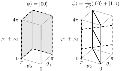
Figure 1: Basic structure of the Husimi function of a factorizing state (left) and a Bell state (right). The full lines indicate the positions of the maxima of the Husimi function. Along the dashed lines and on the gray planes the Husimi function vanishes. The entangled state has a more complex phase space structure than the non-entangled state. For details see Sec. II.

For three spins an expression for the second moment of the Husimi function was given by Sugita in terms of the concurrence between two of the three spins and the so-called 3-tangle coffm00 . As the Husimi function can be defined for an arbitrary number of spins, it is interesting to determine whether and if yes how its second moment is related to entanglement measures for an arbitrary number of spins.

Another motivation for this study arises from the fact that recently phase space methods have been employed to analyze condensed matter systems. In particular the occurrence of a metal-insulator transition in disordered and quasiperiodic systems has been analyzed by means of the inverse participation ratio in phase space wobst03 ; aulba04 . It appears natural to extend these studies to interacting systems. Unfortunately, already the numerical treatment of two particles moving in one dimension is quite demanding. Here, spin systems like the one which we will discuss in Sec. IV present significant advantages. For the interpretation of the phase space properties, it is again interesting to know the relation between the second moment of the Husimi function and the entanglement of the state under consideration.

The phase space approach has occasionally been used in the context of quantum information in the past. The state and time evolution of a quantum computer have been described by means of a discrete Wigner function mique02 ; paz05 . More closely related to the present work is the investigation of the entanglement in bipartite systems on the basis of the Wehrl entropy where each subsystem is described in terms of a sufficiently large spin minte04a . Furthermore, the relation between nonlinear bipartite systems and the classical phase space dynamics has been considered hines05 . In contrast, here we consider the phase space properties of an arbitrary number of distinguishable spins by means of a corresponding number of spin-1/2 coherent states. A single number extracted from such a phase space representation can at best describe entanglement in a very global sense. Therefore, our intention is not to introduce a new quantity to measure entanglement but rather to provide a link between phase space properties and entanglement.

We start in Sec. II by reviewing the phase space representation for spin-1/2 systems and presenting Sugita’s results in a form suitable for the ensuing discussion. In Sec. III the second moment of the Husimi function will be expressed in terms of projectors acting on the Hilbert space and an auxiliary copy. In this way, we make connection to the work by Mintert et al. minte05 which allows us to obtain a relation to concurrences. Finally, in Sec. IV we discuss as an illustrative example the Ising spin chain in presence of a magnetic field perpendicular to the chain axis.

II Phase space for spins

We will restrict our discussion to spin-1/2 systems where the spin-coherent states, the analogue of the coherent states for the harmonic oscillator, are given by radcl71 ; perel86

$$|\vartheta,\varphi\rangle=\cos\left(\frac{\vartheta}{2}\right)|0\rangle+\sin\left(\frac{\vartheta}{2}\right)\mathrm{e}^{i\varphi}|1\rangle$$ (1)

so that each point on the Bloch sphere characterized by the two angles $\vartheta$ and $\varphi$ represents a spin-coherent state. We employ the notation common in quantum information, where $|0\rangle$ and $|1\rangle$ correspond to the eigenstates of the Pauli matrix $\sigma_{z}$ with eigenvalue $+1$ and $-1$, respectively. A coherent state for a system consisting of $N$ distinguishable spins can be expressed as product of coherent states for each of the spins

$$|\mu\rangle=\prod_{i=1}^{N}|\vartheta_{i},\varphi_{i}\rangle\,.$$ (2)

The spin-coherent states (2) enable us to define a positively definite phase space distribution

$$\mathcal{H}(\mu)=\langle\mu|\rho|\mu\rangle$$ (3)

which is the spin analogue of the Husimi- or Q-function familiar from the harmonic oscillator. husim40 ; lee95 In (3), $\rho$ denotes the density matrix of the state for which the phase space distribution is determined.

In order to quantify the extension of a state in phase space, we introduce the second moment of the Husimi function

$$\mathcal{P}=3^{N}\int d\mu\,\mathcal{H}(\mu)^{2}$$ (4)

with the Haar measure $d\mu=\prod_{i=1}^{N}\sin(\vartheta_{i})d\vartheta_{i}d\varphi_{i}/4\pi$. The prefactor is chosen such that a separable state leads to $\mathcal{P}=1$. Up to a factor $(3/2)^{N}$, $\mathcal{P}$ is the inverse participation ratio in phase space. Its inverse measures the extension of the Husimi function in phase space. We note that the second moment of the Husimi function corresponds to the first nontrivial term in the expansion of the Wehrl entropy $\int d\mu\mathcal{H}(\mu)\ln[\mathcal{H}(\mu)]$. wehrl79

To get a feeling for the physical content of the Husimi function $\mathcal{H}$ and its second moment $\mathcal{P}$, we review results obtained for systems containing two or three distinguishable spins. For a pure two-spin state

$$|\psi\rangle=a|00\rangle+b|01\rangle+c|10\rangle+d|11\rangle$$ (5)

with $|a|^{2}+|b|^{2}+|c|^{2}+|d|^{2}=1$ the second moment of the Husimi function is obtained as

$$\mathcal{P}=1-|ad-bc|^{2}\,.$$ (6)

For separable states, one has $ad=bc$ and therefore $\mathcal{P}=1$. On the other hand, the minimal value of the second moment of the Husimi function for systems consisting of two spins is obtained for Bell states with $\mathcal{P}=3/4$. These results indicate the existence of a relation between this phase space quantity and the amount of entanglement.

In order to illustrate the difference between the two cases, it is useful to first consider the Husimi function which, for two spins 1/2, in general is a function of the four angles $\vartheta_{1},\vartheta_{2},\varphi_{1},$ and $\varphi_{2}$. For the factorizing state $|\psi\rangle=|00\rangle$, one obtains the Husimi function

$$\mathcal{H}=\frac{1}{4}\big{(}1+\cos(\vartheta_{1})\big{)}\big{(}1+\cos(\vartheta_{2})\big{)}$$ (7)

while for the Bell state $|\psi\rangle=(|00\rangle+|11\rangle)/\sqrt{2}$ one finds

$$\mathcal{H}=\frac{1}{4}\big{(}1+\cos(\vartheta_{1})\cos(\vartheta_{2})+\sin(\vartheta_{1})\sin(\vartheta_{2})\cos(\varphi_{1}+\varphi_{2})\big{)}\,.$$ (8)

The fact that these Husimi functions depend only on three independent variables allows us to represent their structure in Fig. 1. For the factorizing state $|00\rangle$, the maximum depicted by a full line lies at $\vartheta_{1}=\vartheta_{2}=0$ as should be expected on the basis of (1). The gray areas delimited by the dashed lines indicate the planes at $\vartheta_{1}=\pi$ and $\vartheta_{2}=\pi$ where the Husimi function vanishes. Similarly, for the Bell state in Fig. 1b, the maxima at $\vartheta_{1}=\vartheta_{2}=0$ and $\pi$ indicate the presence of the states $|00\rangle$ and $|11\rangle$. The relative phase between the two states is encoded in the position of the bridges along $\vartheta_{1}=\vartheta_{2}$. The dashed lines again indicate zeroes of the Husimi function. We remark that the independence of the Husimi function on $\varphi_{1}-\varphi_{2}$ is specific to superpositions of the states $|00\rangle$ and $|11\rangle$.

The second moment of the Husimi function (6) for two spins is related to the concurrence hill97

$$\mathcal{C}=|\langle\psi|\sigma_{y}\otimes\sigma_{y}|\psi^{*}\rangle|$$ (9)

where the star denotes the complex conjugate in the eigenbasis of $\sigma_{z}$. An alternative expression, which will be useful in the following, can be obtained by introducing an auxiliary Hilbert space with a copy of the state $|\psi\rangle$. We denote the state in both Hilbert spaces as a column vector $\genfrac{|}{\rangle}{0.0pt}{1}{\psi}{\psi}$. Then the concurrence becomes

$$\mathcal{C}=\left|\left(\left\langle\begin{matrix}0\\ 1\end{matrix}\right|-\left\langle\begin{matrix}1\\ 0\end{matrix}\right|\right)\left(\left\langle\begin{matrix}0\\ 1\end{matrix}\right|-\left\langle\begin{matrix}1\\ 0\end{matrix}\right|\right)\left|\begin{matrix}\psi\\ \psi\end{matrix}\right\rangle\right|$$ (10)

where the first bracket operates in the Hilbert space of the first spin while the second bracket operates in the Hilbert space of the second spin. A more general discussion of expressing the concurrence in terms of projectors can be found in Ref. minte05, . Beyond these formal considerations, such an auxiliary Hilbert space has very recently been employed to directly measure the concurrence of two photons. walbo06

For the general two-spin state (5), the concurrence is given by

$$\mathcal{C}=2|b^{*}c^{*}-a^{*}d^{*}|$$ (11)

so that by comparison of (6) and (11) one immediately obtains the relation

$$\mathcal{P}=1-\frac{\mathcal{C}^{2}}{4}\,.$$ (12)

For three spins, the second moment of the Husimi function can be expressed in terms of the concurrences between two of the three spins $A$, $B$, and $C$ and the 3-tangle $\tau_{ABC}$ coffm00 as

$$\mathcal{P}=1-\frac{1}{4}(\mathcal{C}_{AB}^{2}+\mathcal{C}_{AC}^{2}+\mathcal{C}_{BC}^{2})-\frac{3}{8}\tau_{ABC}\,.$$ (13)

For the generalization to an arbitrary number of spins it is more suggestive to express this result in terms of the concurrences between one spin and the two others as

$$\mathcal{P}=1-\frac{1}{8}(\mathcal{C}_{A(BC)}^{2}+\mathcal{C}_{B(AC)}^{2}+\mathcal{C}_{C(AB)}^{2})\,.$$ (14)

We remark here that the cases of two and three spins are the simplest in the sense that each partition into two subsystems will yield a single concurrence. This is in general no longer true for more than three spins, the case which we are going to address now.

III Second moment of the Husimi function as a projection

For the following considerations it is convenient to express the second moment of the Husimi function (4) in terms of projectors onto symmetric and antisymmetric subspaces. We start by considering a system consisting of a single spin 1/2. The key idea is to express the square in the integrand of (4) in terms of a tensor product of the spin Hilbert space and an auxiliary copy of this Hilbert space. The similarity with the auxiliary Hilbert space introduced in (10) already hints at the possibility of a general relation between the second moment $\mathcal{P}$ and the concurrence $\mathcal{C}$.

In order to distinguish between tensor products of different spins which we note horizontally, the tensor product between one spin Hilbert space and its auxiliary copy will be denoted vertically. The density matrix $\varrho=\rho\otimes\rho$ refers to the tensor product of the density matrices in these two spaces. The second moment of the Husimi function can then be written as

$$\mathcal{P}=\mathrm{Tr}\left(3\int d\mu\varrho\left|\begin{matrix}\mu\\ \mu\end{matrix}\right\rangle\left\langle\begin{matrix}\mu\\ \mu\end{matrix}\right|\right)\,.$$ (15)

By construction, the states $\genfrac{|}{\rangle}{0.0pt}{1}{\mu}{\mu}$ do not contain contributions antisymmetric under exchange of the two Hilbert spaces.

Expressing the projectors in terms of the coherent states (1), one can carry out the integrals over the angles $\vartheta$ and $\varphi$. It turns out that the second moment of the Husimi function can be expressed as

$$\mathcal{P}=\mathrm{Tr}\left(\varrho P_{s}\right)=\langle P_{s}\rangle\,.$$ (16)

Here, $P_{s}=P_{s}^{(1)}+P_{s}^{(2)}+P_{s}^{(3)}$ with

$$P_{s}^{(1)}=\left|\begin{matrix}0\\ 0\end{matrix}\right\rangle\left\langle\begin{matrix}0\\ 0\end{matrix}\right|,\quad P_{s}^{(2)}=\left|\begin{matrix}1\\ 1\end{matrix}\right\rangle\left\langle\begin{matrix}1\\ 1\end{matrix}\right|$$

$$P_{s}^{(3)}=\frac{1}{2}\left(\left|\begin{matrix}0\\ 1\end{matrix}\right\rangle+\left|\begin{matrix}1\\ 0\end{matrix}\right\rangle\right)\left(\left\langle\begin{matrix}0\\ 1\end{matrix}\right|+\left\langle\begin{matrix}1\\ 0\end{matrix}\right|\right)$$ (17)

projects onto the symmetric eigenstates of two qubits while

$$P_{a}=\openone-P_{s}=\frac{1}{2}\left(\left|\begin{matrix}0\\ 1\end{matrix}\right\rangle-\left|\begin{matrix}1\\ 0\end{matrix}\right\rangle\right)\left(\left\langle\begin{matrix}0\\ 1\end{matrix}\right|-\left\langle\begin{matrix}1\\ 0\end{matrix}\right|\right)$$ (18)

projects onto the antisymmetric eigenstate. Expectation values like in (16) are always to be understood in the extended space containing the original Hilbert space as well as a copy.

It is straightforward to generalize this reasoning to more than one qubit because a coherent state according to (2) is defined as a product of coherent states for each qubit. For $N$ qubits, the expression (16) then becomes

$$\mathcal{P}=\langle P_{s}^{\otimes N}\rangle\,.$$ (19)

Making use of the decomposition $\openone=(P_{s}+P_{a})^{\otimes N}$ we can write this expression in the more complicated but useful form

$$\mathcal{P} =\left\langle\openone-(P_{s}+P_{a})^{\otimes N}+P_{s}^{\otimes N}\right\rangle$$ (20)

$$=1-\left\langle\left\{P_{s}^{\otimes N-1}\otimes P_{a}\right\}+\left\{P_{s}^{\otimes N-2}\otimes P_{a}^{\otimes 2}\right\}\right.$$

$$\qquad\qquad\qquad\left.+\dots+\left\{P_{a}^{\otimes N}\right\}\right\rangle\,.$$

The curly braces imply a sum over all different orderings of projection operators. Noting that

$$P_{s}-P_{a}=\left|\begin{matrix}0\\ 0\end{matrix}\right\rangle\left\langle\begin{matrix}0\\ 0\end{matrix}\right|+\left|\begin{matrix}1\\ 1\end{matrix}\right\rangle\left\langle\begin{matrix}1\\ 1\end{matrix}\right|+\left|\begin{matrix}0\\ 1\end{matrix}\right\rangle\left\langle\begin{matrix}1\\ 0\end{matrix}\right|+\left|\begin{matrix}1\\ 0\end{matrix}\right\rangle\left\langle\begin{matrix}0\\ 1\end{matrix}\right|$$ (21)

one can demonstrate the relation

$$\text{Tr}\left(\varrho(P_{s}-P_{a})^{\otimes N}\right)=\text{Tr}(\rho^{2})$$ (22)

which allows us to rewrite (20) as

$$\mathcal{P} =\frac{1}{2}(1+\text{Tr}(\rho^{2}))$$ (23)

$$\quad-\left\langle\left\{P_{s}^{\otimes N-2}\otimes P_{a}^{\otimes 2}\right\}+\left\{P_{s}^{\otimes N-4}\otimes P_{a}^{\otimes 4}\right\}+\dots\right\rangle\,.$$

From (23) it follows that for mixtures all terms in (20) will contribute while for pure states the terms with an odd number of projectors $P_{a}$ onto antisymmetric states are irrelevant. All these contributions clearly vanish because a state $\genfrac{|}{\rangle}{0.0pt}{1}{\psi}{\psi}$ is symmetric under exchange of the Hilbert space and its auxiliary copy.

For the further discussion, we will restrict ourselves to pure states where the second moment of the Husimi function now reads

$$\mathcal{P}=1-\left\langle\left\{P_{s}^{\otimes N-2}\otimes P_{a}^{\otimes 2}\right\}+\left\{P_{s}^{\otimes N-4}\otimes P_{a}^{\otimes 4}\right\}+\dots\right\rangle\,.$$ (24)

In particular, for at most three qubits only one term in the expectation value will contribute, yielding the simple relations (12) and (13).

The expression (24) depends on a linear combination of projectors with equal weight. It represents a special case of a class of operators which can be employed to define a concurrence. Following Ref. minte05, , we introduce the $N$-partite concurrence of a pure state $|\psi\rangle$ describing a system consisting of $N$ spins

$$c_{N}(\psi)=2^{1-N/2}\sqrt{(2^{N}-2)\langle\psi|\psi\rangle^{2}-\sum_{i}\text{Tr}\rho_{i}^{2}}$$ (25)

and find for the second moment of the Husimi function

$$\mathcal{P}=1-\frac{c_{N}(\psi)^{2}}{4}\,.$$ (26)

In (25), $\rho_{i}$ is the reduced density matrix of a subsystem and the sum runs over the $2^{N}-2$ subsystems containing at most $N-1$ spins. Alternatively, one can make use of the relation woott01 ; yu06

$$c_{N}^{2}=2^{2-N}\bar{\mathcal{C}}^{2}$$ (27)

where

$$\bar{\mathcal{C}}=\left(\sum_{\mathrm{partitions}}\sum_{\alpha}\mathcal{C}_{\alpha}^{2}\right)^{1/2}$$ (28)

describes the total length of the concurrence vectors for all partitions of the system into two subsystems. The index $\alpha$ denotes the components of the concurrence vector for a given partition. We thus arrive at the relation between the second moment of the Husimi function and the total length of the concurrence vectors

$$\mathcal{P}=1-\frac{1}{2^{N}}\bar{\mathcal{C}}^{2}\,.$$ (29)

This relation generalizes the results (12) and (13) which are immediately recovered by noting that for two and three spins each concurrence vector contains only one component and that there exist one and three partitions, respectively.

From (29) one can conclude, that entanglement leads to a decrease of the second moment of the Husimi function and thus to a larger spread of the phase space distribution. The relevant measure of the entanglement here is the total length of the concurrence vectors.

It is instructive to determine the second moment $\mathcal{P}$ for two different entangled states, the $N$-qubit GHZ and W states. For the $N$-qubit GHZ state

$$|\text{GHZ}_{N}\rangle=\frac{1}{\sqrt{2}}(|00\cdots 0\rangle+|11\cdots 1\rangle)\,.$$ (30)

one finds

$$\mathcal{P}(|\text{GHZ}_{N}\rangle)=\frac{1}{2}+\frac{1}{2^{N}}\,.$$ (31)

This result makes sense even for only one or two qubits. In the first case, one finds $\mathcal{P}=1$ indicating a “separable” state while in the second case the second moment of the Husimi function of a Bell state is recovered. As the number of qubits increases, $\mathcal{P}$ decreases and approaches the value of $1/2$ in the limit $N\to\infty$.

For the $N$-qubit W state

$$|\text{W}_{N}\rangle =\frac{1}{\sqrt{N}}(|100\cdots 0\rangle+|010\cdots 0\rangle+\cdots)$$ (32)

$$=\frac{1}{\sqrt{N}}\big{[}|1\rangle\otimes|00\cdots 0\rangle+|0\rangle\otimes\sqrt{N-1}|\text{W}_{N-1}\rangle\big{]}$$

one can derive the recursion relation

$$\mathcal{P}(|\text{W}_{N}\rangle)=\frac{(N-1)^{2}}{N^{2}}\mathcal{P}(|\text{W}_{N-1})+\frac{1}{N}\,.$$ (33)

With the initial condition $\mathcal{P}(|\text{W}_{1}\rangle)=1$ one arrives at the solution

$$\mathcal{P}(|\text{W}_{N}\rangle)=\frac{1}{2}+\frac{1}{2N}\,.$$ (34)

As for the GHZ state, the case of two qubits reproduces the second moment of the Husimi function of a Bell state. With an increasing number of qubits, $\mathcal{P}$ decreases and approaches $1/2$ in the limit $N\to\infty$. However, for all $N>2$, the second moment of the Husimi function of a W state is larger than that of a GHZ state. This reflects the fact that the concurrence $c_{N}$ for a GHZ state is larger than that of a W state. carva04 Although $\mathcal{P}$ does not allow to distinguish the different kinds of entanglement present in the two classes of states, a difference is nevertheless visible in the phase space structure which is more extended for a GHZ state.

From the results (31) and (34) one might infer that $\mathcal{P}$ possesses a lower bound of $1/2$. This is however not the case. According to (19), the second moment of the Husimi function for a system consisting of subsystems not entangled among each other is given by the product of the respective $\mathcal{P}$’s of the subsystems. For $N$ pairs of spins in a Bell state, one finds $\mathcal{P}=(3/4)^{N}$ which clearly goes to zero for $N\to\infty$.

IV Ising model in a magnetic field

In the last few years the connection between entanglement and quantum phase transitions has been studied extensively, for example see Refs. oster02, ; osbor02, ; vidal03, ; lator04, ; gunly01, ; fazio05, . In most cases the concurrence has been used as a measure for bipartite entanglement. Taking a different perspective we concentrate on the phase space properties of such a transition. In the previous section we have seen how the concurrence is related to the second moment of the Husimi function. It is therefore interesting to study this phase space quantity for a model exhibiting a quantum phase transition.

As an example we consider a one-dimensional chain of spins 1/2 described by the Hamiltonian

$$H=-J\sum_{i}\left[\sigma_{i}^{z}\sigma_{i+1}^{z}+g\left(\sigma_{i}^{z}\cos\Theta+\sigma_{i}^{x}\sin\Theta\right)\right]\,.$$ (35)

The first term for $J>0$ gives rise to a ferromagnetic coupling between neighboring spins while the second term arises due to a magnetic field which is oriented at an angle $\Theta$ with respect to the $z$-axis. The parameter $g$ describes the ratio between the magnetic field strength and the interaction strength between two neighboring spins. For the case of a transverse magnetic field, $\Theta=\pi/2$, this model undergoes a quantum phase transition at $g=1$. sachd99

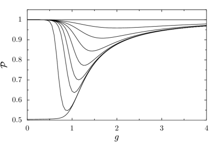
Figure 2: The second moment $\mathcal{P}$ of the Husimi function of a one-dimensional ferromagnetic Ising model with 8 spins and periodic boundary conditions is shown as a function of the coupling constant $g$ for various angles between the $z$-axis and the magnetic field taking the values $\Theta/\pi=0,0.42,0.46,0.48,0.49,0.495,0.4975,0.4995,$ and $0.5$ from the upper to the lower curve.

For $\Theta=0$, the ground state of (35) will be given by a factorizing state either with all spins in state $|0\rangle$ or $|1\rangle$ depending on the sign of $g$. Then, $\mathcal{P}=1$ independent of $g$. For angles $0<\Theta<\pi/2$ and $g\ll 1$, the spins will mostly be in the factorizing state $|0\dots 0\rangle$. However, as $g$ increases, entanglement is build up and the extension of the state in phase spaces increases. Correspondingly, $\mathcal{P}$ will decrease. On the other hand, for $g\gg 1$ the ferromagnetic coupling becomes irrelevant. Then, all spins point in the direction of the magnetic field and $\mathcal{P}$ should reach an asymptotic value of 1. For a transverse magnetic field, $\Theta=\pi/2$, the ground state in the thermodynamic limit, $N\to\infty$, for $g<1$ will be a GHZ state. According to (31), we expect $\mathcal{P}=1/2$. On the other hand, for $g\gg 1$, the asymptotic value $\mathcal{P}=1$ should again be reached.

In Fig. 2, we present numerical results for a system of 8 spins and angles $\Theta$ varying from $0$ to $\pi/2$. From the numerically obtained ground state of (35), the second moment of the Husimi function has been determined by evaluation of (19). The lowest curve represents the case of the transverse Ising model. For $g\ll 1$, one finds a value for $\mathcal{P}$ very close to $1/2$ as expected from (31). For a finite number of spins, $\mathcal{P}$ displays a slight increase even below $g=1$ where in the thermodynamic limit $\mathcal{P}$ is expected to remain at a value of 1/2 before increasing for $g>1$ and reaching $\mathcal{P}=1$ asymptotically. Even for angles $0<\Theta<\pi/2$, the curves in Fig. 2 clearly show that entanglement is built up around $g=1$. The precursor of the quantum phase transition thus manifests itself also in the phase space properties for angles close to $\pi/2$.

We remark that while here we have focussed on the ground state properties, the second moment of the Husimi function can also be determined at finite temperatures. Extensions to the antiferromagnetic coupling and the two-dimensional Ising model are possible within the limits imposed by finite computer resources. schen05

V Conclusions

The relation between the second moment of the Husimi function and the concurrence derived in sugit03 for two and three spins has been generalized to an arbitrary number of spins. The extension of a state in phase space is thus related to its global entanglement properties. Generally, entanglement will imply a delocalization of the Husimi function of a state. Furthermore, the result (26) provides a phase space interpretation of the $N$-partite concurrence (25).

The relation between phase space properties and entanglement has been illustrated by calculating the second moment of the Husimi function for the one-dimensional Ising model with magnetic field. The precursor of a quantum phase transition is clearly seen in the presence of a transverse magnetic field even for a relatively small number of spins. For fields deviating from the transverse direction, the build-up of entanglement close to the critical value of the field can still be observed in the phase space properties.

References

- (1) S. Bose, Phys. Rev. Lett. 91, 207901 (2003).
- (2) D. Burgarth and S. Bose, New J. Phys. 7, 135 (2005) and references therein.
- (3) A. Osterloh, L. Amico, G. Falci, and Rosario Fazio, Nature, 416, 608 (2002).
- (4) T. J. Osborne, and M. A. Nielsen, Phys. Rev. A 66, 032110 (2002).
- (5) G. Vidal, J. I. Latorre, E. Rico, and A. Kitaev, Phys. Rev. Lett. 90, 227902 (2003).
- (6) J. I. Latorre, E. Rico, and G. Vidal, Quantum Inform. Comput. 4, 48 (2004).
- (7) F. Verstraete, D. Porras, and J. I. Cirac, Phys. Rev. Lett. 93, 227205 (2004).
- (8) U. Schollwöck, Rev. Mod. Phys. 77, 259 (2005)
- (9) A. Sugita, J. Phys. A 36, 9081 (2003).
- (10) W. K. Wootters, Quant. Inf. Comp. 1, 27 (2001).
- (11) K. Husimi, Proc. Phys. Math. Soc. Japan 22, 264 (1940).
- (12) H.-W. Lee, Phys. Rep. 259, 264 (1995).
- (13) V. Coffman, J. Kundu, and W. K. Wootters, Phys. Rev. A 61, 052306 (2000).
- (14) A. Wobst, G.-L. Ingold, P. Hänggi, and D. Weinmann, Phys. Rev. B 68, 085103 (2003).
- (15) C. Aulbach, A. Wobst, G.-L. Ingold, P. Hänggi, and I. Varga, New J. Phys. 6, 70 (2004).
- (16) C. Miquel, J. P. Paz, and M. Saraceno, Phys. Rev. A 65, 062309 (2002).
- (17) J. P. Paz, A. J. Roncaglia, and M. Saraceno, Phys. Rev. A 72, 012309 (2005).
- (18) F. Mintert and K. Życzkowski, Phys. Rev. A 69, 022317 (2004).
- (19) A. P. Hines, R. H. McKenzie, and G. J. Milburn, Phys. Rev. A 71, 042303 (2005).
- (20) F. Mintert, A. R. R. Carvalho, M. Kuś, and A. Buchleitner, Phys. Rep. 415, 207 (2005).
- (21) J. M. Radcliffe, J. Phys. A 4, 313 (1971).
- (22) A. Perelomov, Generalized Coherent States and Their Applications (Berlin, 1986).
- (23) A. Wehrl, Rep. Math. Phys. 16, 353 (1979).
- (24) S. Hill and W. K. Wootters, Phys. Rev. Lett. 78, 5022 (1997).
- (25) S. P. Walborn, P. H. Souto Ribeiro, L. Davidovich, F. Mintert, and A. Buchleitner, Nature 440, 1022 (2006)
- (26) C.-S. Yu and H.-S. Song, Phys. Rev. A 73, 022325 (2006).
- (27) A. R. R. Carvalho, F. Mintert, and A. Buchleitner, Phys. Rev. Lett. 93, 230501 (2004).
- (28) R. Fazio and C. Macchiavello, Ann. Phys. (Leipzig) 14, 177 (2005).
- (29) D. Gunlycke, V. M. Kendon, V. Vedral, and S. Bose, Phys. Rev. A 64, 042302 (2001).
- (30) S. Sachdev, Quantum phase transitions (Cambridge, 1999).
- (31) S. Schenk, diploma thesis (Universität Augsburg, 2005).