Diluted maximum-likelihood algorithm for quantum tomography

Abstract

We propose a refined iterative likelihood-maximization algorithm for reconstructing a quantum state from a set of tomographic measurements. The algorithm is characterized by a very high convergence rate and features a simple adaptive procedure that ensures likelihood increase in every iteration and convergence to the maximum-likelihood state. We apply the algorithm to homodyne tomography of optical states and quantum tomography of entangled spin states of trapped ions and investigate its convergence properties.

I Introduction.

Quantum tomography (QT) is a family of methods for reconstructing a state of a quantum system from a variety of measurements performed on many copies of the state. QT is of particular importance for quantum information processing, where it is used to evaluate the fidelity of quantum state preparation, capabilities of quantum information processors, communication channels, and detectors. Theoretically proposed in tomoprop and first experimentally implemented in the early 1990s smi93 , QT has become a standard tool in many branches of quantum information technology.

Aside from the experimental procedure of conducting a set of tomographically complete measurements on a system, QT requires a numerical algorithm for extracting complete information about the state in question from the measurement results. From a variety of algorithms proposed, two main approaches have become popular among experimentalists. One approach is based on linear inversion: because the statistics of the measurement results is a linear function of the density matrix, the latter can be obtained from the former by solving a system of linear equations. Examples are the inverse Radon transformation her80 or the quantum state sampling method sampling , that were almost exclusively used in optical homodyne tomography until recently.

The second approach is maximum-likelihood (MaxLik) quantum state reconstruction, which aims to find, among all possible density matrices, the one which maximizes the probability of obtaining the given experimental data set hradil97 . To date, the maximum-likelihood approach has been applied to various quantum problems from quantum phase estimation Qphase to reconstruction of entangled optical states Rehacek01 ; White01 .

MaxLik reconstruction has several advantages with respect to linear inversion. First, with linear inversion, statistical and systematic errors of the quantum measurements are transferred directly to the density matrix, which may result in unphysical artifacts such as negative diagonal elements. Second, MaxLik allows one to incorporate additional information that may be known about the density matrix into the reconstruction procedure. Third, experimental imperfections (such as detector inefficiencies) can be directly incorporated in to the MaxLik reconstruction procedure.

One approach to quantum MaxLik reconstruction is to express the density matrix as a function of a set of independent parameters, in a way that upholds the positivity and unity-trace constraints for all parameter values. Then one can apply any iterative optimization method to find the set of parameter values that maximize the likelihood. Because the log likelihood function for QT is convex, the optimization problem is well behaved and most iterative optimization methods are guaranteed to converge to the unique solution. This approach was used by James et al. in their work on tomography of optical qubits White01 . In application to homodyne tomography, the method was elaborated by Banaszek et al. B5 and used in an experiment by D’Angelo et al. DAngelo .

Generic numerical optimization methods are often slow when the number of parameters (the square of the Hilbert space dimension) is large. An alternative algorithm described below, which takes advantage of the structure of the MaxLik reconstruction problem and has good convergence properties was proposed by lnp and later adapted to different physical systems such as external degrees of freedom of a photon vortex and the optical harmonic oscillator mll . Thanks to its good properties, this method has been widely used in recent experiments on optical homodyne tomography of both single- and multimode optical states mllapp . Despite its success, no argument guaranteeing monotonic increase of the likelihood in every iteration step has been presented. Although to our knowledge the experimental practice has not yet faced a counterexample, theoretically such counterexamples do exist and there remains a risk that the algorithm could fail for a particular experiment.

In this paper, we propose an iteration which depends on a single parameter $\epsilon$ that determines the “length” of the step in the parameter space. For $\epsilon\to\infty$, the iteration becomes that of Ref. vortex ; mll . On the other hand, we prove that the likelihood will increase in every iteration step for $\epsilon\to 0$. We thus obtain a simple adaptive procedure, which, by choice of parameter $\epsilon$, allows us to find a compromise between the convergence rate and the guarantee on the likelihood increase.

II The nonlinear iterative algorithm.

We now describe the iterative scheme used in Refs. vortex ; mll . A generic tomographic measurement is described by a positive-operator-valued measure (POVM), with the outcome of the $j$’th measurement associated with a specific positive operator $\hat{\Pi}_{j}\geq 0$, with $\sum_{j}\hat{\Pi}_{j}$ normalized to the identity operator. In the case of sharp von Neumann measurements, $\hat{\Pi}_{j}$ is a projection operator.

Let $N$ be the total number of measured quantum systems and $f_{j}$ be the number of occurrences for each measurement result $\hat{\Pi}_{j}$. The likelihood of a particular data set $\{f_{j}\}$ for the quantum state $\hat{\rho}$ is given by $\mathcal{L}(\hat{\rho})=\prod_{j}{\rm pr}_{j}^{f_{j}}$, with

$${\rm pr}_{j}={\rm Tr}[\hat{\Pi}_{j}\hat{\rho}]$$ (1)

being the probability of each outcome.

Our goal is to find the density matrix $\hat{\rho}$ which maximizes the log-likelihood

$$\log\mathcal{L}(\hat{\rho})=\sum_{j}f_{j}\log({\rm pr}_{j}).$$ (2)

As was shown in Ref. hradil97 , a state $\hat{\rho}_{0}$ that maximizes the likelihood (2) obeys a simple nonlinear extremal equation

$$\hat{R}(\hat{\rho}_{0})\hat{\rho}_{0}=\hat{\rho}_{0}\hat{R}(\hat{\rho}_{0})=\hat{\rho}_{0},$$ (3)

where we introduced the state dependent operator

$$\hat{R}(\hat{\rho})=\frac{1}{N}\sum_{j}\frac{f_{j}}{{\rm pr}_{j}}\hat{\Pi}_{j}.$$ (4)

Note that $R(\hat{\rho})$ is a non-negative operator. Following Ref. Fiurasek01 , where a similar method was proposed to estimate an unknown quantum measurement, Eq. (3) can be stated in a slightly different but equivalent form

$$\hat{R}(\hat{\rho}_{0})\hat{\rho}_{0}\hat{R}(\hat{\rho}_{0})=\hat{\rho}_{0}.$$ (5)

For simplicity, we assume that the measurements are sufficient to ensure that there is a unique maximum likelihood state $\hat{\rho}_{0}$.

In the case where the density matrix $\hat{\rho}$ is restricted to matrices that are diagonal, the problem of finding a solution to Eq. (3) can be solved by the well-known expectation-maximization algorithm VardiLee . If $\hat{R}$ is always diagonal in the same basis, expectation-maximization reduces to computing the next iterate according to $\hat{\rho}^{(k+1)}=\hat{R}(\hat{\rho}^{(k)})\hat{\rho}^{(k)}$ in the hope of converging to a fixed point that necessarily satisfies Eq. (3). The expectation-maximization algorithm is guaranteed to increase the likelihood at every iteration step. However, this iteration cannot be used for the quantum problem because without the diagonal restriction, it does not preserve the positivity of the density matrix. A possible remedy is to apply the expectation-maximization iteration to the diagonalized density matrix followed by a unitary transformation of the density matrix eigenbasis Rehacek01 ; Guta .

Refs. vortex ; mll instead propose to base the iterative algorithm on Eq. (5). We choose an initial density matrix such as $\hat{\rho}^{(0)}=\mathcal{N}[\hat{1}]$ (which avoids any initial problems with zero ${\rm pr}_{j}$), and compute the next iterate $\hat{\rho}^{(k+1)}$ from $\hat{\rho}^{(k)}$ using

$$\hat{\rho}^{(k+1)}=\mathcal{N}\left[\hat{R}(\hat{\rho}^{(k)})\hat{\rho}^{(k)}\hat{R}(\hat{\rho}^{(k)})\right],$$ (6)

where $\mathcal{N}$ denotes normalization to trace $1$ and the positivity of the density matrix is explicitly preserved in each step. Hereafter we refer to scheme of Eq. (6) as the “$R\rho R$ algorithm”.

Despite the $R\rho R$ algorithm being a quantum generalization of the well-behaving classical expectation-maximization algorithm, its convergence is not guaranteed in general. This is evidenced by the following counterexample. Assume that we made three measurements on a qubit with a single apparatus with $\hat{\Pi}_{0}=\left|0\right\rangle\!\left\langle 0\right|$, $\hat{\Pi}_{1}=\left|1\right\rangle\!\left\langle 1\right|$, detecting $\left|0\right\rangle$ once and $\left|1\right\rangle$ twice. The measurement is tomographically incomplete because no information is gained about the off-diagonal elements of the density matrix. From Eq. (4), we find $\hat{R}=(\hat{\Pi}_{0}/\rho_{00}+2\hat{\Pi}_{1}/\rho_{11})/3$. Using the uniformly mixed $\hat{\rho}^{(0)}=\hat{\Pi}_{0}/2+\hat{\Pi}_{1}/2$ as a starting point, we obtain, in step 1:

$$\hat{R}=\frac{2}{3}\hat{\Pi}_{0}+\frac{4}{3}\hat{\Pi}_{1};\qquad\hat{\rho}^{(1)}=\hat{\Pi}_{0}/5+4\hat{\Pi}_{1}/5;$$ (7)

and in step 2:

$$\hat{R}=\frac{5}{3}\hat{\Pi}_{0}+\frac{5}{6}\hat{\Pi}_{1};\qquad\hat{\rho}^{(2)}=\hat{\rho}^{(0)}.$$ (8)

The iterations produce a cycle of length two. The second step strictly decreases the likelihood.

III The “diluted” iterative algorithm.

To improve the convergence of the $R\rho R$ iteration let us modify it along the lines used for calculating the mutual entropy of entanglement in mutual , namely by mixing the generator of the nonlinear map (5) with a unity operator

$$\hat{\rho}^{(k+1)}\equiv\hat{I}(\hat{\rho}^{(k)},\epsilon)=\mathcal{N}\left[\frac{\hat{\mathbb{I}}+\epsilon\hat{R}}{1+\epsilon}\hat{\rho}^{(k)}\frac{\hat{\mathbb{I}}+\epsilon\hat{R}}{1+\epsilon}\right],$$ (9)

where $\epsilon$ is a positive number. Loosely speaking, the nonlinear map is diluted and the iteration step is controlled by $\epsilon$. Now let us prove that using the modified algorithm (9), the likelihood is increased in each step if $\epsilon\ll 1$ is sufficiently small.

In the linear approximation with respect to $\epsilon$, we can rewrite Eq. (9) as

$$\hat{\rho}^{(k+1)}=\hat{\rho}^{(k)}+\Delta\hat{\rho}$$ (10)

with

$$\Delta\hat{\rho}=\epsilon(\hat{R}\hat{\rho}^{(k)}+\hat{\rho}^{(k)}\hat{R}-2\hat{\rho}^{(k)}).$$ (11)

To obtain Eqs. (10) and (11), we approximated $(1+\epsilon)^{-2}\approx 1-2\epsilon$ and used the relation

$${\rm Tr}(\hat{R}\hat{\rho})={\rm Tr}(\hat{\rho}\hat{R})=1,$$ (12)

which is a consequence of the definition (4) of $\hat{R}$. The normalization factor $\mathcal{N}$ is $1$ to first order in $\epsilon$.

We now evaluate the likelihood associated with the new state $\hat{\rho}^{(k+1)}$ and compare it to that of $\hat{\rho}^{(k)}$, neglecting terms of second and higher order in $\epsilon$:

$$\log\mathcal{L}(\hat{\rho}^{(k+1)}) = \sum f_{j}\log{\rm Tr}(\hat{\Pi}_{j}\hat{\rho}^{(k+1)})$$

$$= \sum f_{j}\log[{\rm pr}_{j}+{\rm Tr}(\hat{\Pi}_{j}\Delta\hat{\rho})]$$

$$= \sum f_{j}\log{\rm pr}_{j}+\log[1+\frac{1}{{\rm pr}_{j}}{\rm Tr}(\hat{\Pi}_{j}\Delta\hat{\rho})]$$

$$= \log\mathcal{L}(\hat{\rho}^{(k)})+\sum\frac{f_{j}}{{\rm pr}_{j}}{\rm Tr}(\hat{\Pi}_{j}\Delta\hat{\rho})$$

$$= \log\mathcal{L}(\hat{\rho}^{(k)})+{\rm Tr}(\hat{R}\Delta\hat{\rho})$$

$$= \log\mathcal{L}(\hat{\rho}^{(k)})+2\epsilon[{\rm Tr}(\hat{R}\hat{\rho}^{(k)}\hat{R})-1].$$

In the second equality above, we used Eq. (1); in the fourth, the definition (2) of the likelihood and the approximation $\log(1+\alpha)\approx\alpha$ for $\alpha\ll 1$; and in the sixth, the cyclic property of the trace and Eqs. (11) and (12).

We complete the proof by showing that

$$\mathrm{Tr}(\hat{R}\hat{\rho}\hat{R})=\mathrm{Tr}(\hat{R}\hat{\rho}\hat{R})\mathrm{Tr}\hat{\rho}\geq\mathrm{Tr}^{2}(\hat{R}\hat{\rho})=1.$$ (14)

Indeed, the positive density matrix has a positive square root $\hat{\rho}=(\hat{\rho}^{1/2})^{2}$, and thus $\mathrm{Tr}(\hat{R}\rho\hat{R})\mathrm{Tr}\hat{\rho}=(\hat{R}\hat{\rho}^{1/2},\hat{R}\hat{\rho}^{1/2})(\hat{\rho}^{1/2},\hat{\rho}^{1/2})$ and $\mathrm{Tr}^{2}(\hat{R}\hat{\rho})=|(\hat{R}\hat{\rho}^{1/2},\hat{\rho}^{1/2})|^{2}$, where the scalar product of matrices is defined as $(\hat{A},\hat{B})=\sum_{i,j}A^{*}_{ij}B_{ji}={\rm Tr}(\hat{A}^{\dagger}\hat{B})$. Consequently the Cauchy-Schwarz inequality can be applied to yield the inequality in Eq. (14).

We have thus proven that under the application of iterations (9), the likelihood is non-decreasing provided that $\epsilon$ is chosen sufficiently small in every step. Suppose we find a density matrix $\hat{\rho}$ such that there is no $\epsilon>0$ that yields a proper increase in the likelihood when the iteration (9) is applied. Then

$${\rm Tr}(\hat{R}\hat{\rho}\hat{R})=1.$$ (15)

According to Eqs. (12), (14), and the equality condition in the Cauchy-Schwarz inequality, Eq. (15) can be fulfilled if and only if $\hat{R}\hat{\rho}^{1/2}=\hat{\rho}^{1/2}$ or, equivalently, $\hat{R}\hat{\rho}=\hat{\rho}$. The latter equality characterizes the maximum likelihood state, so $\hat{\rho}=\hat{\rho}_{0}$.

Proper use of the diluted iterations requires a strategy for choosing $\epsilon$ at each step. Asymptotic convergence of the diluted iterations may depend on this strategy. As we show in the Appendix, one strategy that converges to $\hat{\rho}_{0}$ is to choose the $\epsilon$ which maximizes the likelihood increase in every iteration. However, this strategy is computationally expensive because it requires solving a one-dimensional optimization problem.

One possible alternative approach is as follows.

• begin with the $R\rho R$ (6) iterations, which are identical to the diluted iterations (9) with $\epsilon\to\infty$. Verify that the likelihood increases in each step.

• In the event the likelihood does not increase and before terminating the iterations, use the diluted iteration (9), trying smaller values of $\epsilon$ to determine whether significant increases in likelihood are still possible. If so, continue the iterations as needed with these smaller values of $\epsilon$.

• When the iterations appear to have converged or stagnated, find the value of $\epsilon$ at which the likelihood increase is maximized and attempt additional iterations using this value. If the likelihood and/or the density matrix does not exhibit significant further changes, one can be sure the iteration sequence has converged to the maximum-likelihood solution.

Another approach is to choose $\epsilon$ randomly according to a distribution with nonzero density in a neighborhood of $0$. To ensure non-decreasing likelihood, each iteration requires repeatedly choosing $\epsilon$ randomly until one is found for which the likelihood increases. The argument in the Appendix can be expanded to show that if $\epsilon$ is chosen in this way, then the iteration has a non-zero probability of escaping from any non-maximum likelihood density matrix.

We note again that in all practical cases studied so far the $R\rho R$ algorithm exhibited good convergence and monotonic increase of the likelihood. The diluted iteration may become necessary for low-dimensional systems where the nonlinear $R\rho R$ iteration may “overshoot”. Characterizing the situations where this can happen is an open problem.

Finally, let us mention that in some tomography schemes, one or more POVM elements (measurement channels) $\Pi_{j}$ are not accessible and, consequently, $\hat{G}\equiv\sum_{j}\hat{\Pi}_{j}$ may not be normalizable to the unity operator on the reconstruction subspace. Then the extremal map (5) should be replaced by $\hat{G}^{-1}\hat{R}(\hat{\rho}_{0})\hat{\rho}_{0}\hat{R}(\rho_{0})\hat{G}^{-1}=\hat{\rho}_{0}$ to avoid biased results, see e.g. Rehacek01 . Obviously, the corresponding iterative procedure can be diluted in a similar way as was done with the original $R\rho R$ algorithm.

IV Examples

First, consider the counterexample discussed above. A simple numerical test shows that replacing the $R\rho R$ iteration by (9) warrants convergence for any finite $\epsilon$; the likelihood monotonically increases for $\epsilon\lesssim 25.7$.

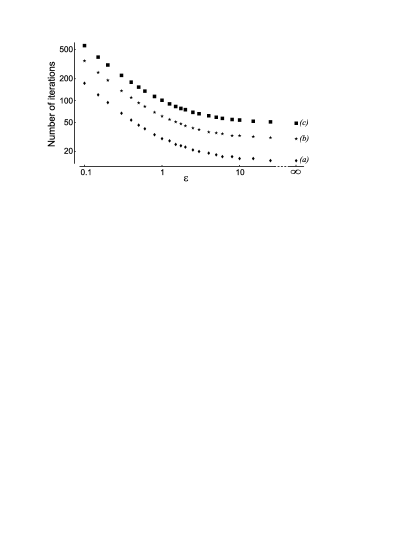
Figure 1: Iterations required for homodyne tomography data. The number of iterations required for convergence as a function of $\epsilon$. Results for three tolerances are shown: $10^{-3}$ (a), $10^{-5}$ (b) and $10^{-7}$ (c). The rightmost column represents the $R\rho R$ algorithm ($\epsilon\to\infty$). The dataset is the same as that used in Ref. mll : 14,153 quadrature samples of the state approximating a coherent superposition of the vacuum and the single-photon states.

Second, we studied the dataset of 14,153 points obtained in the experiment on homodyne tomography of the coherent superposition of the vacuum and the single-photon Fock state catalysis . This is the same dataset as that analyzed in Ref. mll . This reference discusses the specifics of application of the likelihood-maximization procedure to continuous-variable measurements. We studied the dependence of the convergence speed on the parameter $\epsilon$.

The Hilbert space was restricted to 14 photons. We first ran the iterations for a very long time until the density matrix and the likelihood no longer changed. In this way, we obtained the density matrix $\hat{\rho}_{0}$ that maximizes the likelihood for this dataset with high accuracy (limited by the floating point representation).

We then re-initialized the density matrix and ran the diluted $R\rho R$ algorithm with various values of $\epsilon$. We repeated the iterations until the pairwise difference between all matrix elements of $\hat{\rho}^{(k)}$ and $\hat{\rho}_{0}$ was below a pre-selected tolerance for each matrix element. Three tolerance values were investigated: $10^{-3}$, $10^{-5}$ and $10^{-7}$. The numerical experiment was conducted on a 2.8-GHz Pentium 4 computer tradenames . The code was written in Delphi tradenames . Each iteration took about 0.3 s.

The result of this experiment is shown in Fig. 1. The $R\rho R$ algorithm showed monotonic likelihood increase and converged to the set tolerances within 15, 30, and 49 iterations, respectively. The convergence rate of the diluted algorithm improves with increasing $\epsilon$ and approached that of the $R\rho R$ algorithm for large values of $\epsilon$. One sign of systematic overshoot of the $R\rho R$ algorithm would be a minimum in the three curves of Fig. 1 at $\epsilon<\infty$. We did not observe such an effect.

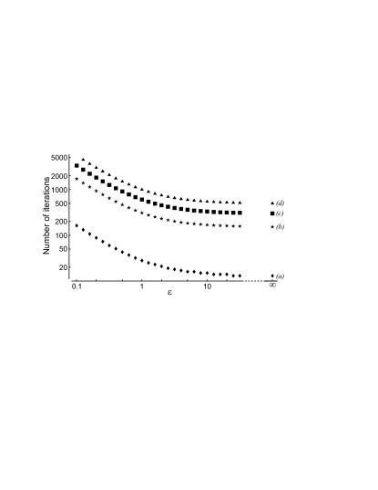
Figure 2: Required iterations for ion-qubit tomography data. See the caption of Fig. 1 for an explanation of the axes and interpretation of the curves. The tolerances used are $10^{-2}$ (a), $10^{-3}$ (b), $10^{-4}$ (c) and $10^{-7}$ (d). The underlying data was used in the analysis for reichle:qc2006a .

Third, we considered a dataset consisting of 21,832 individual experiments with four ion qubits. The goal of the experiment was to purify one entangled pair of ions from two reichle:qc2006a . In order to determine the fidelity of the purified pair and for the purpose of checking that the experiment did not introduce spurious entanglement, incomplete state tomography was used. Specifically, each tomographic measurement involved first determining the number of qubits in state $\left|0\right\rangle$ among the first pair of qubits and then performing a pair of $\pi/2$ pulses at various phases on the second pair of qubits (the purified pair) before determining its number of ions in state $\left|0\right\rangle$. Repetition of these combinations of pulses and measurements suffices for determining the fidelity of the purified entangled state. The actual measurements involve counting the number of photons scattered from an ion pair. This number has a Poissonian distribution whose mean depends on the number of ions in state $\left|0\right\rangle$. Thus, each experiment results in two counts, one from each measurement. Every combination of counts can be associated with a measurement operator of a POVM that also depends on the phases in the pair of $\pi/2$ pulses. Although we cannot determine the density matrix of the complete four-qubit state $\hat{\rho}$ with these measurements, there is sufficient information to deduce the density matrix $\hat{\rho}^{\prime}$ obtained from $\hat{\rho}$ by phase decohering the first pair of qubits in the logical basis and then symmetrizing each pair of qubits. The symmetrization process is equivalent to randomly switching the qubits in each pair. The diluted $R\rho R$ iteration with the appropriate POVMs preserves the decohered and symmetrized form of density matrices. Starting from the completely mixed initial state, it converges to the maximum likelihood solution for $\hat{\rho}^{\prime}$. The code for the ion-qubit tomography was written in R Rref and required about .3 s per iteration on a 1.6 GHz Pentium 4 laptop. The behavior of the iterations is shown in Fig. 2 and is similar to the behavior of the iterations for the homodyne tomography shown in Fig. 1. Again, no sign of overshoot was detected in these curves.

In summary, we have proposed an iterative likelihood-maximization procedure for quantum tomography, which is applicable when the $R\rho R$ iteration does not monotonically increase the likelihood. We have found the sufficient condition under which the iterations converge to the maximum-likelihood solution. The new algorithm has been tested on two sets of experimental data.

Appendix A Convergence of diluted iterations

Consider the diluted iterations (9). For any fixed $\epsilon$, we cannot exclude the possibility that the iteration stagnates, even if the likelihoods continue to increase. The problem is that the direction of change in $\hat{\rho}$ for small $\epsilon$, which is computed as a fixed function of $\hat{\rho}$, may differ substantially from the direction of steepest ascent. Although the likelihood is guaranteed to increase for sufficiently small $\epsilon$, the direction of change could become increasingly parallel to surfaces of constant likelihood, thus leading to an iteration that never reaches the maximum likelihood solution $\hat{\rho}_{0}$. Alternatively, if $\epsilon$ is held fixed, the iterations could converge into a limit cycle or a more complicated limit set, thus avoiding $\hat{\rho}_{0}$.

Here we show that if at each step, $\epsilon$ is chosen to maximize the likelihood increase, the iterations converge to $\hat{\rho}_{0}$ in the limit. To see this, we first notice that $\hat{R}(\hat{\rho})$ is continuous as a function of $\hat{\rho}$ on the set $S$ of density matrices for which the likelihood is not $0$. This is because, if $\hat{\rho}\in S$, then ${\rm pr}_{j}>0$ for all $j$ with $f_{j}>0$. It follows that the iterate $\hat{I}$ defined by Eq. (9) is also a continuous function of the density matrix and $\epsilon\geq 0$.

The initial density matrix $\hat{\rho}^{(0)}$ (the completely mixed state) is in $S$ because, for any $j$, ${\rm pr}_{j}(\hat{\rho}^{(0)})={\rm Tr}[\hat{\Pi}_{j}\hat{\rho^{(0)}}]\propto{\rm Tr}[\hat{\Pi}_{j}]>0$. The choice of $\epsilon$ guarantees that the likelihood is non-decreasing, so each subsequent iterate $\hat{\rho}^{(k)}$ must be in $S$ as well. The sequence $\hat{\rho}^{(k)}$ is bounded and must thus have at least one limit point $\hat{\rho}_{l}$, which also belongs to the interior of $S$.

Suppose that $\hat{\rho}_{l}\not=\hat{\rho}_{0}$. As we showed in the text, this implies that the likelihood of $\hat{I}(\hat{\rho}_{l},\epsilon)$ strictly increases for sufficiently small $\epsilon$. In particular, there is a $\delta>0$ and an $\epsilon$, such that the likelihood increase at $\hat{\rho}_{l}$ is at least $\delta$. Because the likelihood increase is also a continuous function of $\hat{\rho}$ and $\epsilon$ on a neighborhood of $\hat{\rho}_{l}$, there is a (possibly smaller) neighborhood $S_{\delta}$ in which the maximum likelihood increase exceeds $\delta/2$. Because $\hat{\rho}_{l}$ is a limit point, one can choose an iterate $\hat{\rho}^{(k)}$ in $S_{\delta}$ so that its likelihood is within (say) $\delta/4$ of that of $\hat{\rho}_{l}$. Then the next iterate’s likelihood exceeds that of $\hat{\rho}_{l}$ by at least $\delta/4$. Since the likelihood is non-decreasing, and by continuity, future iterates cannot have $\hat{\rho}_{l}$ as a limit point, contradicting the assumption on $\hat{\rho}_{l}$. We conclude that $\hat{\rho}_{l}=\hat{\rho}_{0}$, as desired.

References

- (1) R. G. Newton and B. L. Young, Ann. Phys. (New York), 49, 393 (1968); J. L. Park and W. Band, Found. Phys., 1, 211 (1971); W. Band, and J. L. Park, Am. J. Phys., 47, 188 (1979); Found. Phys., 1, 133 (1970); Found. Phys., 1, 339 (1971); J. Bertrand and P. Bertrand, Found. Phys. 17, 397 (1987); K. Vogel and H. Risken, Phys. Rev. A 40, 2847 (1989).
- (2) D. T. Smithey, M. Beck, M G. Raymer and A. Faridani, Phys. Rev. Lett. 70, 1244 (1993); D. T. Smithey,M. Beck, J. Cooper, M. G. Raymer and A. Faridani, Physica Scripta T48, 35 (1993).
- (3) G. T. Herman, Image Reconstruction from Projections: The Fundamentals of Computerized Tomography (Academic Press, New York, 1980).
- (4) G. M. D’Ariano, C. Macchiavello, and M. G. A. Paris, Phys. Rev. A 50, 4298 (1994); G. M. D’Ariano, M. G. A. Paris, M. F. Sacchi, in Quantum State Estimation, M. Paris and J. Rehacek (Eds.), Lect. Notes Phys. 649 (Springer, Berlin Heidelberg, 2004); U. Leonhardt et al., Opt. Commun. 127, 144 (1996).
- (5) Z. Hradil, Phys. Rev. A 55, R1561 (1997).
- (6) Y. Vardi and D. Lee, J. R. Statist. Soc B 55, 569 (1993).
- (7) J. Řeháček, Z. Hradil, M. Zawisky, S. Pascazio, H. Rauch, and J. Peřina, Phys. Rev. A 60, 473 (1999).
- (8) J. Řeháček, Z. Hradil, and M. Ježek, Phys. Rev. A 63, 040303(R) (2001).
- (9) D.F.V. James, P.G. Kwiat, W.J. Munro, and A.G. White, Phys. Rev. A 64, 052312 (2001).
- (10) K. Banaszek, G. M. D’Ariano, M. G. A. Paris, M. F. Sacchi, Phys. Rev. A 61, 010304(R) (1999).
- (11) M. D’Angelo, A. Zavatta, V. Parigi, M. Bellini, quant-ph/0602150
- (12) Z. Hradil, J. Řeháček, J. Fiurášek, and M. Ježek in Quantum State Estimation edited by M. Paris and J. Řeháček, Lect. Notes Phys. 649 (Springer, Berlin Heidelberg, 2004).
- (13) G. Molina-Terriza, A. Vaziri, J. Rehacek, Z. Hradil, A. Zeilinger, Phys. Rev. Lett. 92, 167903 (2004).
- (14) A. I. Lvovsky, J. Opt. B: Q. Semiclass. Opt. 6 S556 (2004).
- (15) A. Ourjoumtsev, R. Tualle-Brouri, P. Grangier, Phys. Rev. Lett. 96, 213601 (2006); Science 312, 83 (2006); J. S. Neergaard-Nielsen et al., quant-ph/0602198; S. A. Babichev, B. Brezger, A. I. Lvovsky, Phys. Rev. Lett. 92, 047903 (2004); S. A. Babichev, J. Appel, A. I. Lvovsky, Phys. Rev. Lett. 92, 193601 (2004).
- (16) J. Fiurášek, Phys. Rev. A 64, 024102 (2001).
- (17) L. M. Artilles, R. D. Gill, and M. I. Guta, J. R. Statist. Soc B 67, 109 (2005).
- (18) J. Rehacek, Z. Hradil, Phys. Rev. Lett. 90, 127904 (2003).
- (19) A. I. Lvovsky and J. Mlynek, Phys. Rev. Lett. 88 250401 (2002).
- (20) R. Reichle, D. Leibfried, E. Knill, J. Britton, R. B. Blakestad, J. D. Jost, C. Langer, R. Ozeri, S. Seidelin and D. J. Wineland, Nature 443, 838 (2006).
- (21) The use of trade names is for informational purposes only and does not imply endorsement by NIST.
- (22) The R Project for Statistical Computing, http://www.r-project.org.