Efficient classical simulation of the approximate quantum Fourier transform

Abstract

We present a method for classically simulating quantum circuits based on the tensor contraction model of Markov and Shi (quant-ph/0511069). Using this method we are able to classically simulate the approximate quantum Fourier transform in polynomial time. Moreover, our approach allows us to formulate a condition for the composability of simulable quantum circuits. We use this condition to show that any circuit composed of a constant number of approximate quantum Fourier transform circuits and $\log$ depth circuits with limited interaction range can also be efficiently simulated.

One of the most useful ways of investigating the power, and limitations, of quantum computation is to identify classes of quantum algorithms which can be efficiently simulated on a classical computer. A well-known example of such a class are circuits composed of Clifford group operations, which are shown by the Gottesman-Knill theorem gottesman to be efficiently simulable. Recently a number of new methods for simulating quantum computation have appeared jozsa ; markov ; briegel ; us , both for the circuit model and the measurement-based model of quantum computation. Unlike the Gottesman-Knill theorem which is based on restricting the set of allowed gates, all these new methods rely on the topology (the ‘graph’ of connections) of the simulated circuit. In particular two of these new methods, due to Jozsa jozsa and Markov and Shi markov , both use the formalism of tensor contraction for simulations in the quantum circuit model, which is the focus of this paper.

We base our approach on Markov and Shi’s formalism, which has the advantage of being able to simulate generalised quantum dynamics and mixed states (this would be particularly useful in simulating noisy gates), as well as working directly with the natural graph of the circuit. Using this approach, we show how the approximate quantum Fourier transform (AQFT) can be efficiently simulated on a classical computer (i.e. simulated in a time polynomial in the number of input qubits). Additionally, our method allows us to formulate a simple condition for the composability of two simulable circuits. That is, if the simulation procedures for two circuits obey a particular condition, we are assured that the composed circuit (created by connecting the outputs of one to the inputs of the other) will also be efficiently simulable. We use this condition to show that any circuit composed of constant number of AQFT circuits and $\log$ depth quantum circuits with bounded interaction range can be efficiently simulated on a classical computer. Obviously, this implies that the AQFT can be efficiently simulated when applied to any state produced by such circuits.

Simulating Quantum Computation In order to simulate a quantum computation, we first associate a graph with the circuit in the obvious way, representing each input qubit, gate, and output qubit by a vertex, and each wire by an edge (e.g. a two-qubit gate would correspond to a vertex of degree four). Next, we label each edge with a different index (i,j,k, etc.). Each index ranges over four possible values, corresponding to the four components of a qubit’s density operator. Finally, to each vertex we associate a tensor describing the operation performed at that point. This tensor has indices corresponding to all edges connected to that vertex (so that its rank is equal to the degree of the vertex). For clarity, we use raised indices to denote output wires, and lowered indices to denote input wires.

Following Markov and Shi’s approach markov , we associate tensors with basic circuit elements as follows, using the operator basis $e_{i}=\{|0\rangle\langle 0|,|0\rangle\langle 1|,|1\rangle\langle 0|,|1\rangle\langle 1|\}$ for single qubits, and $e_{ij}=e_{i}\otimes e_{j}$ for two qubits:

1. Inputting a qubit in state $\rho$:

   $$\lx@xy@svg{\hbox{\raise 0.0pt\hbox{\kern 0.0pt\hbox{\ignorespaces\ignorespaces\ignorespaces\hbox{\vtop{\kern 0.0pt\offinterlineskip\halign{\entry@#!@&&\entry@@#!@\cr&&&\crcr}}}\ignorespaces{\hbox{\kern 0.0pt\raise 0.0pt\hbox{\hbox{\kern-3.0pt\raise 0.0pt\hbox{\hbox{\kern 3.0pt\raise 0.0pt\hbox{$\textstyle{}$}}}}}}}{\hbox{\kern 14.22636pt\raise 0.0pt\hbox{\hbox{\kern-10.17015pt\raise-1.18056pt\hbox{$\textstyle{\rho}$}}}}}{\hbox{\kern 28.45273pt\raise 0.0pt\hbox{\hbox{\kern-1.72256pt\raise 5.0pt\hbox{$\textstyle{i}$}}}}}\ignorespaces\ignorespaces\ignorespaces\ignorespaces{}{\hbox{\lx@xy@droprule}}\ignorespaces{}{\hbox{\lx@xy@droprule}}{\hbox{\lx@xy@droprule}}{\hbox{\kern 42.6791pt\raise 0.0pt\hbox{\hbox{\kern-3.0pt\raise 0.0pt\hbox{\hbox{\kern 3.0pt\raise 0.0pt\hbox{$\textstyle{\ignorespaces\ignorespaces\ignorespaces\ignorespaces}$}}}}}}}\ignorespaces\ignorespaces\ignorespaces\ignorespaces{}{\hbox{\lx@xy@droprule}}\ignorespaces{}{\hbox{\lx@xy@droprule}}{\hbox{\lx@xy@droprule}}\ignorespaces}}}}\ignorespaces\qquad T^{i}=\mathrm{tr}(e^{\dagger}_{i}\rho) \textstyle{\rho} \textstyle{i} \textstyle{\rho} \textstyle{i}$$ (1)

2. Performing a single-qubit operation $\rho\rightarrow G[\rho]$:

   $$\lx@xy@svg{\hbox{\raise 0.0pt\hbox{\kern 0.0pt\hbox{\ignorespaces\ignorespaces\ignorespaces\hbox{\vtop{\kern 0.0pt\offinterlineskip\halign{\entry@#!@&&\entry@@#!@\cr&&&&\crcr}}}\ignorespaces{\hbox{\kern 0.0pt\raise 0.0pt\hbox{\hbox{\kern-3.0pt\raise 0.0pt\hbox{\hbox{\kern 3.0pt\raise 0.0pt\hbox{$\textstyle{}$}}}}}}}{\hbox{\kern 14.22636pt\raise 0.0pt\hbox{\hbox{\kern-1.72256pt\raise 5.0pt\hbox{$\textstyle{i}$}}}}}\ignorespaces\ignorespaces\ignorespaces\ignorespaces{}{\hbox{\lx@xy@droprule}}\ignorespaces{}{\hbox{\lx@xy@droprule}}{\hbox{\lx@xy@droprule}}{\hbox{\kern 28.45273pt\raise 0.0pt\hbox{\hbox{\kern 0.0pt\raise 0.0pt\hbox{$\textstyle{\lx@xy@svgnested{\hbox{\raise 0.0pt\hbox{\kern 6.93127pt\hbox{{\hbox{\kern-6.93127pt\raise 0.0pt\hbox{\hbox{\kern 3.00003pt\raise-3.41666pt\hbox{$\textstyle{G}$}}}}}\ignorespaces\ignorespaces\ignorespaces\ignorespaces\ignorespaces{\hbox{\lx@xy@droprule}}\ignorespaces\ignorespaces\ignorespaces\ignorespaces\ignorespaces\ignorespaces{\hbox{\lx@xy@droprule}}\ignorespaces\ignorespaces\ignorespaces\ignorespaces\ignorespaces\ignorespaces{\hbox{\lx@xy@droprule}}\ignorespaces\ignorespaces\ignorespaces\ignorespaces\ignorespaces{\hbox{\lx@xy@droprule}}}}}}}$}}}}}\ignorespaces\ignorespaces\ignorespaces\ignorespaces{}{\hbox{\lx@xy@droprule}}\ignorespaces{}{\hbox{\lx@xy@droprule}}{\hbox{\lx@xy@droprule}}{\hbox{\kern 56.54164pt\raise 0.0pt\hbox{\hbox{\kern-2.34525pt\raise 6.94444pt\hbox{$\textstyle{j}$}}}}}\ignorespaces\ignorespaces\ignorespaces\ignorespaces{}{\hbox{\lx@xy@droprule}}\ignorespaces{}{\hbox{\lx@xy@droprule}}{\hbox{\lx@xy@droprule}}{\hbox{\kern 70.768pt\raise 0.0pt\hbox{\hbox{\kern-3.0pt\raise 0.0pt\hbox{\hbox{\kern 3.0pt\raise 0.0pt\hbox{$\textstyle{\ignorespaces\ignorespaces\ignorespaces\ignorespaces}$}}}}}}}\ignorespaces\ignorespaces\ignorespaces\ignorespaces{}{\hbox{\lx@xy@droprule}}\ignorespaces{}{\hbox{\lx@xy@droprule}}{\hbox{\lx@xy@droprule}}\ignorespaces}}}}\ignorespaces\qquad T^{j}_{i}=\mathrm{tr}(e^{\dagger}_{i}G[e_{j}]) \textstyle{i} \textstyle{G} \textstyle{j} \textstyle{i} \textstyle{G} \textstyle{j}$$ (2)

3. Performing a two-qubit operation $\rho\rightarrow G^{\prime}[\rho]$

   $$\lx@xy@svg{\hbox{\raise 0.0pt\hbox{\kern 0.0pt\hbox{\ignorespaces\ignorespaces\ignorespaces\hbox{\vtop{\kern 0.0pt\offinterlineskip\halign{\entry@#!@&&\entry@@#!@\cr&&&&\\&&&&\crcr}}}\ignorespaces{\hbox{\kern 0.0pt\raise 0.0pt\hbox{\hbox{\kern-3.0pt\raise 0.0pt\hbox{\hbox{\kern 3.0pt\raise 0.0pt\hbox{$\textstyle{}$}}}}}}}{\hbox{\kern 14.22636pt\raise 0.0pt\hbox{\hbox{\kern-1.72256pt\raise 5.0pt\hbox{$\textstyle{i}$}}}}}\ignorespaces\ignorespaces\ignorespaces\ignorespaces{}{\hbox{\lx@xy@droprule}}\ignorespaces{}{\hbox{\lx@xy@droprule}}{\hbox{\lx@xy@droprule}}{\hbox{\kern 28.45273pt\raise 0.0pt\hbox{\hbox{\kern 5.00002pt\raise-4.19444pt\hbox{$\textstyle{\hphantom{G^{\prime}}}$}}}}}\ignorespaces\ignorespaces\ignorespaces\ignorespaces{}{\hbox{\lx@xy@droprule}}\ignorespaces{}{\hbox{\lx@xy@droprule}}{\hbox{\lx@xy@droprule}}\ignorespaces\ignorespaces{\hbox{\kern 33.45274pt\raise-17.23032pt\hbox{\hbox{\kern 0.0pt\raise-4.19444pt\hbox{$\textstyle{G^{\prime}}$}}}}}\ignorespaces\ignorespaces\ignorespaces\ignorespaces\ignorespaces{\hbox{\lx@xy@droprule}}\ignorespaces\ignorespaces\ignorespaces\ignorespaces\ignorespaces{\hbox{\lx@xy@droprule}}\ignorespaces\ignorespaces\ignorespaces\ignorespaces\ignorespaces{\hbox{\lx@xy@droprule}}\ignorespaces\ignorespaces\ignorespaces\ignorespaces\ignorespaces{\hbox{\lx@xy@droprule}}{\hbox{\kern 62.08159pt\raise 0.0pt\hbox{\hbox{\kern-2.76042pt\raise 5.0pt\hbox{$\textstyle{k}$}}}}}\ignorespaces\ignorespaces\ignorespaces\ignorespaces{}{\hbox{\lx@xy@droprule}}\ignorespaces{}{\hbox{\lx@xy@droprule}}{\hbox{\lx@xy@droprule}}{\hbox{\kern 76.30795pt\raise 0.0pt\hbox{\hbox{\kern-3.0pt\raise 0.0pt\hbox{\hbox{\kern 3.0pt\raise 0.0pt\hbox{$\textstyle{\ignorespaces\ignorespaces\ignorespaces\ignorespaces}$}}}}}}}\ignorespaces\ignorespaces\ignorespaces\ignorespaces{}{\hbox{\lx@xy@droprule}}\ignorespaces{}{\hbox{\lx@xy@droprule}}{\hbox{\lx@xy@droprule}}{\hbox{\kern 0.0pt\raise-34.46062pt\hbox{\hbox{\kern-3.0pt\raise 0.0pt\hbox{\hbox{\kern 3.0pt\raise 0.0pt\hbox{$\textstyle{}$}}}}}}}{\hbox{\kern 14.22636pt\raise-34.46062pt\hbox{\hbox{\kern-2.34525pt\raise 6.94444pt\hbox{$\textstyle{j}$}}}}}\ignorespaces\ignorespaces\ignorespaces\ignorespaces{}{\hbox{\lx@xy@droprule}}\ignorespaces{}{\hbox{\lx@xy@droprule}}{\hbox{\lx@xy@droprule}}{\hbox{\kern 28.45273pt\raise-34.46062pt\hbox{\hbox{\kern 5.00002pt\raise-4.19444pt\hbox{$\textstyle{\hphantom{G^{\prime}}}$}}}}}\ignorespaces\ignorespaces\ignorespaces\ignorespaces{}{\hbox{\lx@xy@droprule}}\ignorespaces{}{\hbox{\lx@xy@droprule}}{\hbox{\lx@xy@droprule}}{\hbox{\kern 62.08159pt\raise-34.46062pt\hbox{\hbox{\kern-1.59029pt\raise 5.0pt\hbox{$\textstyle{l}$}}}}}\ignorespaces\ignorespaces\ignorespaces\ignorespaces{}{\hbox{\lx@xy@droprule}}\ignorespaces{}{\hbox{\lx@xy@droprule}}{\hbox{\lx@xy@droprule}}{\hbox{\kern 76.30795pt\raise-34.46062pt\hbox{\hbox{\kern-3.0pt\raise 0.0pt\hbox{\hbox{\kern 3.0pt\raise 0.0pt\hbox{$\textstyle{\ignorespaces\ignorespaces\ignorespaces\ignorespaces}$}}}}}}}\ignorespaces\ignorespaces\ignorespaces\ignorespaces{}{\hbox{\lx@xy@droprule}}\ignorespaces{}{\hbox{\lx@xy@droprule}}{\hbox{\lx@xy@droprule}}\ignorespaces}}}}\ignorespaces\qquad T^{kl}_{ij}=\mathrm{tr}(e^{\dagger}_{ij}G^{\prime}[e_{kl}]) \textstyle{i} \textstyle{G^{\prime}} \textstyle{k} \textstyle{j} \textstyle{l} \textstyle{i} \textstyle{G^{\prime}} \textstyle{k} \textstyle{j} \textstyle{l}$$ (3)

4. Obtaining a measurement result corresponding to a generalised measurement (POVM) operator $E$:

   $$\lx@xy@svg{\hbox{\raise 0.0pt\hbox{\kern 0.0pt\hbox{\ignorespaces\ignorespaces\ignorespaces\hbox{\vtop{\kern 0.0pt\offinterlineskip\halign{\entry@#!@&&\entry@@#!@\cr&&\crcr}}}\ignorespaces{\hbox{\kern 0.0pt\raise 0.0pt\hbox{\hbox{\kern-3.0pt\raise 0.0pt\hbox{\hbox{\kern 3.0pt\raise 0.0pt\hbox{$\textstyle{}$}}}}}}}{\hbox{\kern 14.22636pt\raise 0.0pt\hbox{\hbox{\kern-1.72256pt\raise 5.0pt\hbox{$\textstyle{i}$}}}}}\ignorespaces\ignorespaces\ignorespaces\ignorespaces{}{\hbox{\lx@xy@droprule}}\ignorespaces{}{\hbox{\lx@xy@droprule}}{\hbox{\lx@xy@droprule}}{\hbox{\kern 28.45273pt\raise 0.0pt\hbox{\hbox{\kern 0.0pt\raise 0.0pt\hbox{$\textstyle{\lx@xy@svgnested{\hbox{\raise 0.0pt\hbox{\kern 11.97919pt\hbox{{\hbox{\kern-6.97919pt\raise 0.0pt\hbox{\hbox{\kern 3.00003pt\raise-3.41666pt\hbox{$\textstyle{E}$}}}}}\ignorespaces\ignorespaces\ignorespaces\ignorespaces\ignorespaces{\hbox{\lx@xy@droprule}}\ignorespaces\ignorespaces\ignorespaces\ignorespaces\ignorespaces\ignorespaces{\hbox{\lx@xy@droprule}}\ignorespaces\ignorespaces\ignorespaces\ignorespaces\ignorespaces\ignorespaces{\hbox{\lx@xy@droprule}}\ignorespaces\ignorespaces\ignorespaces\ignorespaces\ignorespaces\ignorespaces{\hbox{\lx@xy@drawline@}}\ignorespaces\ignorespaces\ignorespaces\ignorespaces\ignorespaces{\hbox{\lx@xy@drawline@}}}}}}}$}}}}}\ignorespaces\ignorespaces\ignorespaces\ignorespaces{}{\hbox{\lx@xy@droprule}}\ignorespaces{}{\hbox{\lx@xy@droprule}}{\hbox{\lx@xy@droprule}}\ignorespaces}}}}\ignorespaces\qquad T_{j}=\mathrm{tr}(Ee_{j}) \textstyle{i} \textstyle{E} \textstyle{i} \textstyle{E}$$ (4)

5. Discarding a qubit, or obtaining an unspecified measurement result:

   $$\lx@xy@svg{\hbox{\raise 0.0pt\hbox{\kern 0.0pt\hbox{\ignorespaces\ignorespaces\ignorespaces\hbox{\vtop{\kern 0.0pt\offinterlineskip\halign{\entry@#!@&&\entry@@#!@\cr&&\crcr}}}\ignorespaces{\hbox{\kern 0.0pt\raise 0.0pt\hbox{\hbox{\kern-3.0pt\raise 0.0pt\hbox{\hbox{\kern 3.0pt\raise 0.0pt\hbox{$\textstyle{}$}}}}}}}{\hbox{\kern 14.22636pt\raise 0.0pt\hbox{\hbox{\kern-1.72256pt\raise 5.0pt\hbox{$\textstyle{i}$}}}}}\ignorespaces\ignorespaces\ignorespaces\ignorespaces{}{\hbox{\lx@xy@droprule}}\ignorespaces{}{\hbox{\lx@xy@droprule}}{\hbox{\lx@xy@droprule}}{\hbox{\kern 28.45273pt\raise 0.0pt\hbox{\hbox{\kern 0.0pt\raise 0.0pt\hbox{$\textstyle{\lx@xy@svgnested{\hbox{\raise 0.0pt\hbox{\kern 8.00003pt\hbox{{}\ignorespaces\ignorespaces\ignorespaces\ignorespaces\ignorespaces{\hbox{\lx@xy@droprule}}\ignorespaces\ignorespaces\ignorespaces\ignorespaces\ignorespaces\ignorespaces{\hbox{\lx@xy@droprule}}\ignorespaces\ignorespaces\ignorespaces\ignorespaces\ignorespaces\ignorespaces{\hbox{\lx@xy@droprule}}\ignorespaces\ignorespaces\ignorespaces\ignorespaces\ignorespaces\ignorespaces{\hbox{\lx@xy@drawline@}}\ignorespaces\ignorespaces\ignorespaces\ignorespaces\ignorespaces{\hbox{\lx@xy@drawline@}}}}}}}$}}}}}\ignorespaces\ignorespaces\ignorespaces\ignorespaces{}{\hbox{\lx@xy@droprule}}\ignorespaces{}{\hbox{\lx@xy@droprule}}{\hbox{\lx@xy@droprule}}\ignorespaces}}}}\ignorespaces\qquad T_{j}=\mathrm{tr}(e_{j}) \textstyle{i} \textstyle{i}$$ (5)

Note that these examples can easily be extended to apply to joint input states or measurements, gates acting on more qubits, or gates with different numbers of inputs and outputs. Tensors could even be introduced to represent non-physical (i.e. not completely positive) linear operations if desired.

Once a tensor with the appropriate indices has been assigned to each vertex, taking their product and summing over all indices will yield the probability of obtaining the specified measurement result. This process is illustrated below for the simple circuit shown in fig. 1, in which a two qubit unitary gate $G[\rho]=U\rho U^{\dagger}$ acts on the separable input state $\rho_{1}\otimes\rho_{2}$, and the probability $p$ of the first qubit being found in the state $\left|{0}\right\rangle$ is obtained.

$$p = \sum_{ijkl}T^{i}\,T^{j}\,T^{kl}_{ij}\,T_{k}\,T_{l}$$

$$= \sum_{ijkl}\mathrm{tr}(e^{\dagger}_{i}\rho_{1})\mathrm{tr}(e^{\dagger}_{j}\rho_{2})\mathrm{tr}(e^{\dagger}_{kl}Ue_{ij}U^{\dagger})\mathrm{tr}(|0\rangle\langle 0|e_{k})\mathrm{tr}(e_{l})$$

$$= \sum_{kl}\mathrm{tr}(e^{\dagger}_{kl}U(\rho_{1}\otimes\rho_{2})U^{\dagger})\mathrm{tr}((|0\rangle\langle 0|\otimes I)e_{kl})$$

$$= \mathrm{tr}\left((|0\rangle\langle 0|\otimes I)U(\rho_{1}\otimes\rho_{2})U^{\dagger}\right)$$

Figure 1: The graph and tensors associated with a simple example circuit described below, in which a two-qubit unitary gate acts on the state $\rho_{1}\otimes\rho_{2}$, and the first qubit is measured to be in state $\left|{0}\right\rangle$.

Note that in cases where we wish to measure many output qubits, it may be prohibitive to calculate the probability of all possible output strings (as there are exponentially many possibilities). Instead, a closer analogy to the real quantum computation would be to sample from the probability distribution to obtain a particular random measurement result. This can be achieved by computing the probability of measurement outcomes for the first qubit (with the measurement results for all other qubits unspecified) and randomly selecting a result, then computing the joint probability of measurement results for the second qubit with the chosen result on the first qubit, and randomly selecting one, and so on until a particular measurement result has been selected for each qubit.

The problem with summing over all tensor indices at the same time (as written in equation (Efficient classical simulation of the approximate quantum Fourier transform)) is that there are exponentially many terms, making the computation very slow. To avoid this, we ‘contract’ the tensors together one at a time, breaking the joint sum into a series of separate sums. In each step of the computation we replace two existing tensors with a new tensor obtained by summing over any repeated indices (e.g. $T^{kl}_{ij}T^{no}_{lm}\rightarrow T^{kno}_{ijm}$). We repeat this procedure until we are left with a single tensor with no free indices, which is the desired probability. The aim is to order the contractions so that we never generate tensors with too many indices during this process.

In Markov and Shi’s paper, they describe this contraction process by an ordering on the edges of the graph (i.e. on index summations). However here we take a different approach, in which the contraction process is described by a sequence of sets of vertices $\cal{S}$ $=(s^{1},\ldots,s^{N})$ - each of which corresponds to a particular tensor that is generated during the computation. This allows us to formulate a condition for efficient simulation of composite circuits.

The tensor corresponding to a set of vertices $s$ is that generated by contracting together all initial tensors corresponding to vertices in $s$. In each step of the contraction process we take two existing tensors and generate a new one, so each set $s^{i}\in\cal{S}$ is either the union of two previous sets, or one previous set and a vertex, or two vertices. Denoting the set of all vertices by $V$:

$$s^{i}=\{t_{1}^{i}\cup t_{2}^{i}\}\quad\mbox{where}\quad\begin{array}[]{l}\mbox{either}\;\;\>t_{j}^{i}=s^{k}\>,\>k<i\>,\\ \mbox{or}\quad\quad\>t_{j}^{i}=\{v\}\>,\>v\in V.\end{array}$$ (7)

The calculation of the probability is done in $N$ steps, where in step $i$ we compute a new tensor by summing over all indices corresponding to edges connecting $t_{1}^{i}$ to $t_{2}^{i}$. For the computation to be complete, we require that the final set $s^{N}=V$. Note that sampling from the output probability distribution for many qubits as described above only requires changing the measurement operators applied to the outputs, and hence each run can use the same graph and contraction sequence ${\cal S}$.

The computational difficulty of the simulation is determined by the maximal rank of the tensors generated during the computation. For each $s^{i}$ in $\cal{S}$ we therefore define $E^{i}$ as the number of edges that connect vertices in $s^{i}$ to vertices outside $s^{i}$, which is exactly the rank of the tensor corresponding to $s^{i}$. The simulation corresponding to the sequence $\cal S$ will be an efficient one if $E^{max}=\max_{i}E^{i}=O(\log n)$. This condition assures us that the maximal number of components for each tensor we compute is $O(\mathrm{poly}(n))$. Furthermore, the maximal number of terms summed over when computing each component must also be $O(\mathrm{poly}(n))$, as the two sets $t_{1}^{i}$ and $t_{2}^{i}$ which are combined to form $s^{i}$ can only connect on at most $E^{max}=O(\log n)$ edges.

A class of circuits that is easy to simulate efficiently using this approach is that of log-depth circuits with bounded interaction range (i.e. involving $d=O(\log n)$ timesteps, in which gates act on qubits at most a constant distance $r$ apart). To simulate such circuits, we number all vertices involving qubit 1 first (i.e. gates, inputs and outputs on the upper horizontal line of the circuit), then all vertices involving qubit 2 that are not already included, and so on until we have numbered all the vertices. The sequence $\mathcal{S}$ is then composed of sets containing increasing numbers of vertices in this ordering (e.g. $(\{v^{1}\},\{v^{1},v^{2}\},\ldots)$. It is easy to see that for such simulations, $E^{\max}\leq dr=O(\log n)$. The efficient simulability of such circuits has previously been shown in markov ; us . Furthermore, it was shown by Jozsa jozsa , using a slightly different approach , that the same strategy will work for any circuit in which each qubit line is touched (or crossed) by at most $O(\log n)$ gates.

Simulating the Approximate Quantum Fourier Transform. An important new example of a circuit which can be efficiently simulated by the above scheme is the approximate quantum Fourier transform (AQFT). An efficient circuit for the exact Fourier transform nielsen consists of a sequence of $(n-1)$ ‘ladder circuits’ of decreasing size. The $l^{\mathrm{th}}$ ladder circuit is composed of a Hadamard gate on the $l^{\mathrm{th}}$ qubit, followed by ($n-l$) conditional phase gates connecting qubit $l$ to qubits $l+1,\ldots n$ respectively. These conditional phase gates have the form $R_{k}=exp(\pi i/2^{k})|11\rangle\langle 11|$, where $k$ is the distance over which the gate acts.

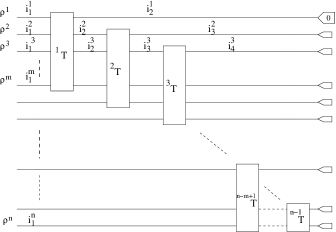
Figure 2: The general structure of the circuit calculating the approximate quantum Fourier transform, showing a measurement of $\left|{0}\right\rangle$ on the first output qubit. Each box corresponds to a ladder circuit, with internal gates as shown in fig.3.

However, it was noted by Coppersmith coppersmith that in many case an exact Fourier transform is not necessary, and that a very good approximation can be obtained by omitting all gates $R_{k}$ with $k>m$ (i.e. gates that act over a large distance, and generate only small phase rotations). In what follows, we take $m=\log(n/\epsilon)$, yielding an error in the final state of $O(\epsilon)$. Furthermore this approximate quantum fourier transform is sufficient for the most useful application of the algorithm - for estimating periodicity, and hence for use in Shor’s factoring algorithm shor . Barenco et al. barenco proved that the AQFT will yield the same probability of success as the exact periodicity-finding algorithm after $O(n^{3}/m^{3})$ runs. A diagram of the AQFT circuit is given in fig. 2. Note that in this circuit, the output qubits occur in reverse order to the inputs (i.e. starting at the bottom).

Figure 3: The gates composing a ladder circuit, consisting of a Hadamard gate and then $m-1$ controlled rotation gates. Note that the last few ladder circuits are actually slightly smaller, although they have the same form.

In order to classically simulate the $AQFT$ circuit we cannot use the same simple ordering $\mathcal{S}$ used for the log-depth circuits above, as $O((\log n)^{2})$ gates cross each qubit line. This leads to tensors with $n^{O(\log\,n)}$ elements, that cannot be computed in polynomial time. Instead, we choose the following contraction ordering: We first contract together all of the tensors corresponding to gates in the first ladder circuit (in any order), then we proceed to do the same for the second ladder circuit, and so on, until we have one combined tensor for each ladder circuit (i.e. until $\mathcal{S}$ contains sets corresponding to the vertices in each ladder circuit). Since there are at most $m=O(\log n)$ two-qubit gates in each ladder circuit, all the tensors we generate have at most $O(\log n)$ indices.

Next we combine the ladder circuits and their associated inputs and outputs, one by one in descending order, until we have contracted together all the remaining tensors. First, we take the tensor for the top ladder circuit and contract it with all the tensors of input and output vertices to which it is connected, in order from top to bottom (i.e. $i_{1}^{1}$ to $i_{1}^{m}$ and $i_{2}^{1}$) . Then we contract this new tensor with the tensor for the second ladder circuit, and again contract it with any input or output vertices to which it is connected (i.e. $i_{1}^{m+1}$ and $i_{2}^{2}$). We continue to contract each new tensor with that of the next ladder circuit, and its inputs and outputs vertices, until all tensors have been included - and thus we have computed the probability of the chosen measurement result.

Note that in each stage of the contraction process, the new tensors we generate only have at most $E^{max}=O(\log n)$ free indices - hence storing and computing these tensors requires only polynomial time and memory space. We have therefore proved that the approximate quantum fourier transform can be efficiently simulated classically.

So far we have assumed that the input to the AQFT circuit is a product state of $n$ qubits (although this need not be a computational basis state). A way to generalize this set of possible input states is to identify classes of efficiently simulable circuits that can be connected to the inputs of the AQFT circuit such that the composed circuit is also efficiently simulable. In the next section, we therefore consider the simulability of composed circuits.

Simulating composed circuits. Consider two efficiently simulable circuits, $A$ and $B$, that we join together to form a composed circuit $C$ by connecting the output wires of $A$ to the input wires of $B$ (for simplicity we assume that both are $n$ qubit circuits, our discussion can be easily generalized to the case where only some of the inputs and output connect). How can we tell if the composed circuit $C$ is efficiently simulable?

In what follows we will use the subscripts $a$ and $b$ to label objects belonging to circuits $A$ and $B$ respectively. Let us also denote the set of output vertices of $A$ by $V_{a}^{out}$ and the set of input vertices of $B$ by $V_{b}^{in}$. Given efficient simulations of $A$ and $B$, $C$ will be efficiently simulable if the following condition holds: For any subset $\omega_{a}=\{v_{a,i_{1}}^{out}\ldots v_{a,i_{k}}^{out}\}$ of $V_{a}^{out}$, if there is a set $s_{a}\in{\cal S}_{a}$ which includes exactly this subset of output vertices (i.e. $s_{a}\cap V_{a}^{out}=\omega_{a}$), then there is a set $s_{b}\in{\cal S}_{b}$ containing exactly the same subset of input vertices (i.e. $s_{b}\cap V_{b}^{in}=\{v_{b,i_{1}}^{in}\ldots v_{b,i_{k}}^{in}\}$).

To prove that this condition is sufficient, we first decompose all the sets in ${\cal S}_{a}$ containing output vertices into their output and non-output components, writing $s^{ij}_{a}=\omega^{i}_{a}\cup\mu^{ij}_{a}$, where $\omega^{i}_{a}\in V_{a}^{out}$ denotes a particular set of output vertices, and $\mu^{ij}_{a}$ denotes a corresponding set of non-output vertices. Similarly, we decompose each set $s_{b}\in{\cal S}_{b}$ containing input vertices in the same way into a set of input vertices $\eta^{i}_{b}$ and their associated non-input vertices $\mu^{ij}_{b}$, such that $s^{ij}_{b}=\eta^{i}_{b}\cup\mu^{ij}_{b}$.

From our simulation procedure it is clear that any two sets in a sequence are either disjoint or are such that one includes the other. It is also clear that the order in which two disjoint sets are constructed is arbitrary (we can choose which set to construct first). Therefore, by re-labelling and re-ordering the sets in $\mathcal{S}_{a}$, we can ensure that all sets not containing output vertices occur first, and that the remaining sets $s^{ij}_{a}$ occur in the order of increasing $i$ and then increasing $j$ (e.g. $s^{11}_{a},s^{12}_{a},s^{13}_{a},s^{21},\ldots$), and similarly for $\mathcal{S}_{b}$ and the input vertices. Furthermore, our composability condition ensures that we can find sequences of this form, such that the output vertices in $\omega^{i}_{a}$ connect precisely with the input vertices in $\eta^{i}_{b}$.

We construct a sequence of sets $\mathcal{S}_{c}$ for the combined circuit $C$ as follows: Starting with circuit $A$, we first include all sets from $\mathcal{S}_{a}$ that do not involve input vertices, then do the same for $\mathcal{S}_{b}$. The next set we include is $\mu^{11}_{a}\cup\mu^{11}_{b}$, in which the first output from $A$ is contracted with an input of $B$ (yielding the union of two non-output sets). We proceed to evolve this set in $A$ by including $\mu^{1j}_{a}\cup\mu^{11}_{b}$ for $j=2,\ldots j^{\max}_{1}$. After this, we shift to evolving circuit $B$, by including sets $\mu^{1j^{\max}_{1}}_{a}\cup\mu^{1k}_{b}$ for $k=1,\ldots k^{\max}_{1}$. Then, beginning with $\mu^{21}_{a}\cup\mu^{21}_{b}$, we repeat the above procedure for $i=2,\ldots,i^{max}$, by including $\mu^{ij}_{a}\cup\mu^{i1}_{b}$ for $j=1,\ldots j^{\max}_{i}$, then $\mu^{ij^{\max}_{2}}_{a}\cup\mu^{ik}_{b}$ for $k=1,\ldots j^{\max}_{i}$, until all vertices in the combined circuit have been included.

The key point is that at any stage in the above process the sets we construct are either identical to a set in the original sequences, or composed of a union of two such sets with some input and output vertices discarded (i.e those across which the circuit is connected). It is therefore clear that $E^{\max}_{c}\leq(E_{a}^{\max}+E_{b}^{\max})$, and hence when both $E_{a}^{\max}$ and $E_{b}^{\max}$ are $O(\log n)$, the simulation process defined by ${\cal S}_{c}$ is an efficient one.

These results can be generalised to apply to any constant number of efficiently simulable circuits connected in series. In such cases, the combined circuit will be efficiently simulable when the above composability condition is satisfied across each circuit boundary.

From the simulation procedures for the AQFT circuit and log-depth limited range circuits given above, we see that both the input and output vertices are included sequentially from bottom to top (i.e. $\omega_{i}=\{v_{1}^{out},\ldots,v_{i}^{out}\}$ and $\eta_{i}=\{v_{1}^{in},\ldots,v_{i}^{in}\}$). As each output set from one circuit corresponds exactly to an input set for the other, these two circuits obey our composability condition. Furthermore, with $\omega_{i}$ and $\eta_{i}$ defined as above, their simulation sequences do not need to be rearranged before they are composed. By joining these two circuits together, we can classically simulate the approximate quantum Fourier transform on any input state that can be produced by log-depth circuit involving limited range interactions.

Because the outputs of the AQFT circuit occur in reverse order, attaching a circuit afterwards is more tricky, but can be achieved by flipping the attached circuit vertically. In order to satisfy the composability condition, tensors in the flipped circuit must still be contracted from top to bottom, but this can easily be achieved for both types of circuit considered here (since the original circuits are also simulable with a bottom to top contraction ordering). We therefore conclude that any circuit which is composed of a constant number of AQFT and log-depth limited range circuits can be simulated efficiently on a classical computer.

- (1) D. Gottesman. quant-ph/9807006.
- (2) R. Jozsa, quant-ph/0603163.
- (3) I. Markov and Y. Shi, quant-ph/0511069.
- (4) M. Van den Nest, W. D r, G. Vidal, H. J. Briegel, quant-ph/0608060.
- (5) N. Yoran and A. J. Short, Phys. Rev. Lett. 96, 170503 (2006).
- (6) M. A. Nielsen and I. L. Chuang, Quantum Computation and Quantum Information (Cambridge University Press, 2000).
- (7) D. Coppersmith, IBM research report RC 19642 (1994).
- (8) P. W. Shor, Proceedings, Annual Symposium on Computer Science (IEEE , Los Alamitos, CA 1996).
- (9) A. Barenco, A. Ekert, K-A. Souminen and P. Törmä, Phys. Rev. A. 54, 139 (1996).