Approximate locality for quantum systems on graphs

Abstract

In this Letter we make progress on a longstanding open problem of Aaronson and Ambainis [Theory of Computing 1, 47 (2005)]: we show that if $A$ is the adjacency matrix of a sufficiently sparse low-dimensional graph then the unitary operator $e^{it{A}}$ can be approximated by a unitary operator $U(t)$ whose sparsity pattern is exactly that of a low-dimensional graph which gets more dense as $|t|$ increases. Secondly, we show that if $U$ is a sparse unitary operator with a gap $\Delta$ in its spectrum, then there exists an approximate logarithm $H$ of $U$ which is also sparse. The sparsity pattern of $H$ gets more dense as $1/\Delta$ increases. These two results can be interpreted as a way to convert between local continuous-time and local discrete-time processes. As an example we show that the discrete-time coined quantum walk can be realised as an approximately local continuous-time quantum walk. Finally, we use our construction to provide a definition for a fractional quantum fourier transform.

In physics the word locality admits many possible interpretations. In quantum field theory and condensed matter physics locality is understood as the clustering of correlations endnote18 ; Weinberg (1996); Peskin and Schroeder (1995); Fredenhagen (1985); Lieb and Robinson (1972); Hastings (2004); Cramer and Eisert (2006). In quantum information theory the quantum circuit model Nielsen and Chuang (2000); Preskill (1998) reigns supreme as the final arbiter of locality where it is natural to define the nonlocality of a physical process to be the minimal number of fundamental two-qubit quantum gates required to simulate the process up to some prespecified error endnote19 . The central role the quantum circuit model plays in assessing the nonlocal “cost” of a physical process strongly motivates us to quantify the relationship between the notions of locality accepted in other branches of physics and the quantum gate cost of quantum information theory.

Thus, we appear to have at least two different interpretations of the word locality for quantum systems: on one hand we have the clustering of many-particle physics, and on the other we have the gate cost of quantum information theory. From a physical perspective it is in intuitively clear that there should be a strong relationship between these two definitions. After all, dynamical clustering implies a bound on the speed of information transmission. Indeed, for many particle systems there are now results quantifying this relationship: a low-dimensional system which exhibits dynamical clustering can be simulated by a constant-depth quantum circuit Osborne (2006).

However, for the case of scalar and spinor quantum particles hopping on finite graphs an explication of the connections between the clustering-type interpretation of locality and the quantum-circuit type interpretation has yet to be completed. An investigation of the graph setting was initiated by Aaronson and Ambainis Aaronson and Ambainis (2005), who established the canonical analogues of the clustering and quantum-circuit definitions of locality. The main questions remaining are now to quantify the relationship between the quantum-circuit locality (what Aaronson and Ambainis call “$Z$-locality” and “$C$-locality”) and the clustering-type interpretation (called “$H$-locality”) for these systems.

The objective of this Letter is to provide a (not necessarily optimal) equivalence between the notions of locality introduced in Aaronson and Ambainis (2005), thus partially resolving one of their longstanding conjectures: we establish that a graph-local continuous-time process can be written (“discretised”) as a product of discrete-time processes (“quantum gates”). Conversely, we show how to compute an approximately local logarithm for a unitary gate which is local on some graph $G$. In other words, we show how to construct a local continuous-time process $\mathcal{C}$ associated with a local discrete-time quantum process $\mathcal{D}$ such that $\mathcal{D}$ may be realised by sampling $\mathcal{C}$ at appropriate intervals.

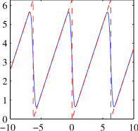
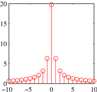
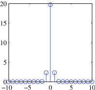
Figure 1: Smoothing out the sawtooth to improve convergence of fourier coefficients: in the first figure the original sawtooth wave is shown in red, along with the smoothed version in blue. In the second figure the absolute values of ($2\pi$ times) the fourier coefficients of the original sawtooth are shown. Note the slow convergence of this sequence. Finally, in the third figure the fourier coefficients of the smoothed sawtooth are shown. Note the improved convergence of the sequence.

All the quantum systems we consider in this Letter are naturally associated with a finite graph $G=(V,E)$, where $V$ is a set of $n$ vertices and $E$ a set of edges. We write $v\sim w$ if $(v,w)\in E$. We summarise this connectivity information using the adjacency matrix $A$, which has matrix elements given by $A_{v,w}=1$ if $v\sim w$ and $A_{v,w}=0$ otherwise. For two vertices $v,w\in V$ we let $\operatorname{dist}(v,w)$ denote the graph-theoretical distance — the length of the shortest path connecting $v$ and $w$, with respect to the edge set $E$. Let $M\in\mathcal{M}_{n}(\mathbb{C})$ be an $n\times n$ matrix. The sparsity pattern $A$ of $M$ is the $n\times n$ $\{0,1\}$-matrix given by: $A_{j,k}=0$ if $M_{j,k}=0$ and $A_{j,k}=1$ if $M_{j,k}\not=0$. It is sometimes convenient in the sequel to arbitrarily assign directions (arrows) to the edges of $G$. In this case we write $e^{+}$ (respectively, $e^{-}$) for the vertex at the beginning (respectively, end) of $e$. Finally, we denote by $D(G)$ the maximum degree of $G$, which is the maximum number of edges which are incident to any vertex in $G$.

There is a canonical way to associate a Hilbert space $\mathcal{H}_{V}$ with a finite graph $G$ with vertex set $V$: we use vertices to label a basis of quantum states, so that $\mathcal{H}_{V}\equiv\langle|v\rangle\,|\,v\in V\rangle$ — this is the Hilbert space of a scalar quantum particle constrained to live on the vertices of $G$.

We now recall the definitions of locality introduced by Aaronson and Ambainis Aaronson and Ambainis (2005) for a quantum particle on a graph. Note that the definitions we present here are not as general as those introduced in Aaronson and Ambainis (2005): Aaronson and Ambainis include the possibility of an extra internal degree of freedom. While, for clarity, we ignore this extra internal degree of freedom it is straightforward to extend our results to cover the more general case.

Definition 1.

A unitary matrix $U$ is said to be $Z$-local on $G$ if $U_{j,k}=0$ whenever $j\not=k$ and $(j,k)\not\in E$.

Definition 2.

A unitary matrix $U$ is said to be $C$-local on $G$ if:

1. the basis states $|v\rangle$ can be partitioned into subsets $\mathcal{P}_{1},\mathcal{P}_{2},\ldots,\mathcal{P}_{q}$ such that $U_{j,k}=0$ whenever $|j\rangle$ and $|k\rangle$ belong to distinct subsets $P_{l}$; and

2. for each $j$, all basis states in $\mathcal{P}_{j}$ are either from the same vertex or from two adjacent vertices.

Definition 3.

A unitary matrix $U$ is said to be $H$-local on $G$ if $U=e^{iH}$ for some hermitian matrix $H$ with $\|H\|_{\infty}\leq\pi$ such that $H_{j,k}=0$ whenever $j\not=k$ and $(j,k)\not\in E$.

The first result we prove in this Letter shows how an $H$-local unitary operator may be written as a product of $C$-local unitary operators. This result is entirely standard and is a straightforward corollary of the sparse hamiltonian lemma of Aharonov and Ta-Shma (2003). We sketch a proof for completeness.

Proposition 4.

Let $H$ be the adjacency matrix of a finite graph $G$. Then $e^{itH}$ may be approximated by a product of $c|t|D(G)$ $C$-local unitary operators, where $c$ is some constant. Because a product of $C$-local unitary operators is $Z$-local on some graph related to $G$ an $H$-local unitary operator is approximately $Z$-local on some graph $G^{\prime}$ related to $G$, which gets denser as $|t|$ increases.

Proof.

The idea behind the proof is as follows. We first write $H=\sum_{j=1}^{D(G)+1}h_{j}$, where $h_{j}=\sum_{e\in\mathcal{C}_{j}}\alpha_{e}^{(j)}$, $\alpha_{e}^{(j)}=|e^{+}\rangle\langle e^{-}|+\text{h.c.}$, and $[\alpha_{e}^{(j)},\alpha_{f}^{(j)}]=0$ (this decomposition follows from a colouring of the edges provided by Vizing’s theorem Vizing (1964): we denote by $\mathcal{C}_{j}$ the set of edges with the same colour). Then we use the Lie-Trotter formula to approximate $e^{itH}$ by powers of $U_{\delta}=(e^{i\delta h_{1}}e^{i\delta h_{2}}\cdots e^{i\delta h_{m}})(e^{i\delta h_{m}}\cdots e^{i\delta h_{1}})$:

$$\|U_{\delta}^{\lfloor\frac{|t|}{2\delta}\rfloor}-e^{itH}\|_{\infty}\leq O(m\Lambda\delta+m\Lambda^{3}|t|\delta^{2}),$$ (1)

where $m=D(G)+1$ and $\Lambda=\max_{j}\|h_{j}\|_{\infty}\leq 2$, where the inequality for $\|h_{j}\|$ follows straightforwardly from, for example, Geršgorin’s circle theorem Horn and Johnson (1990). Finally, we observe that $e^{i\delta h_{j}}$ is a $C$-local unitary operator, for each $j=1,2,\ldots,m$. ∎

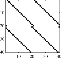
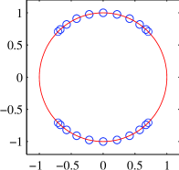
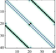
Figure 2: The coined quantum walk $U$ on a ring with $20$ sites. The first figure shows the sparsity pattern of $U$. The second figure shows the spectrum of $U$ with a gap clearly evident. The third figure shows the absolute values of the matrix elements of the logarithm $H$ of $U$ constructed in the proof of Proposition 5. Note the rapid decay of the matrix elements away from the original nonzero entries of $U$.

Proposition 5.

Let $U$ be a unitary matrix whose sparsity pattern $A$ is the adjacency matrix of a digraph $G$. If the arguments $\theta$ of all of the eigenvalues $e^{i\theta}$ of $U$ satisfy $\theta\in[0,2\pi)\setminus(\alpha,\beta)$, with $\Delta=|\alpha-\beta|$, then there exists a unitary matrix $V$ which is $H$-local on a graph $G^{\prime}$ given by the sparsity pattern of $A(G)^{k}$ where $k=c/(\epsilon^{2}\Delta)$, for some constant $c$, such that $\|U-V\|_{\infty}\leq\epsilon$.

Proof.

We begin by writing $U$ in its eigenbasis:

$$U=\sum_{j=1}^{n}e^{i\phi_{j}}|j\rangle\langle j|,$$ (2)

where $|j\rangle$ are the eigenvectors of $U$ and we choose $\phi_{j}\in[0,2\pi)$. By multiplying by an overall unimportant phase $e^{i\zeta}\mathbb{I}$ we can set the zero of angle to arrange for a gap in the spectrum $\operatorname{spec}(U)$ of $U$ to lie over the origin. Such a gap always exists for finite dimensional unitary operators, but not necessarily for infinite operators.

We want to find a hermitian matrix $H$ so that $U=e^{iH}$. We call this the effective hamiltonian for $U$. One such hamiltonian is simply given by

$$H=\sum_{j=1}^{n}\phi_{j}|j\rangle\langle j|.$$ (3)

While this expression is perfectly well-defined, it is very hard to see any kind of sparsity/local structure in $H$. To overcome this we’ll find an alternative expression for $H$ defined by Eq. (3) as a power series in $U$. To do this we suppose that

$$H=\sum_{k=-\infty}^{\infty}c_{k}U^{k},$$ (4)

and we solve for the coefficients $c_{k}$: we equate the coefficient of $|j\rangle\langle j|$ on both sides to find

$$\phi_{j}=\sum_{k=-\infty}^{\infty}c_{k}e^{ik\phi_{j}}.$$ (5)

Hence, if we can find $c_{k}$ such that

$$\theta=\sum_{k=-\infty}^{\infty}c_{k}e^{ik\theta},$$ (6)

for all $\theta\in[0,2\pi)$ then we are done. (Recall that we’ve arranged it so there are no eigenvalues of $U$ on the point $\theta=0$.) To solve for $c_{k}$ we integrate both sides of Eq. (6) with respect to $\theta$ over the interval $[0,2\pi)$ against $\frac{1}{2\pi}e^{-il\theta}$, for $l\in\mathbb{Z}$:

$$\frac{1}{2\pi}\int_{0}^{2\pi}\theta e^{-il\theta}\,d\theta=\frac{1}{2\pi}\sum_{k=-\infty}^{\infty}c_{k}\int_{0}^{2\pi}e^{i(k-l)\theta}\,d\theta.$$ (7)

Thus we learn that the $c_{k}$ are nothing but the fourier coefficients of the periodic sawtooth function $f(\theta+2\pi l)=\theta$, $\theta\in[0,2\pi)$, $l\in\mathbb{Z}$:

$$c_{k}=\begin{cases}\pi,\quad k=0\\ \frac{i}{k},\quad k\not=0.\end{cases}$$ (8)

Now we know the formula for $c_{k}$ we substitute this into Eq. (4):

$$H=\sum_{k=-\infty}^{\infty}\left(\pi\delta_{k,0}+\frac{i(1-\delta_{k,0})}{k}\right)U^{k},$$ (9)

and truncate the series at some cutoff $k\leq K$. If we assume the sparsity pattern of $U$ describes a sufficiently sparse graph $G$ then $U^{k}$ will also describe a sparse graph for any constant $k$ endnote20 , and, as a consequence, the truncated series representation for $H$ would also describe a sparse graph.

Unfortunately we cannot do this: the sawtooth wave has a jump discontinuity and hence the fourier series is only conditionally convergent. Thus it is impossible to truncate the series without a serious error.

The way to proceed is to assume that we have some further information, namely, that $U$ has a gap $\Delta$ in its spectrum. The eigenvalues of $U$ lie on the unit circle in the complex plane so what we mean here is that there is a continuous arc in the unit circle which subtends an angle $\Delta$ where there are no eigenvalues of $U$. We arrange, by multiplying by an unimportant overall phase, for this gap to be centred on the origin.

The idea now is to exploit the existence of the gap to provide a more useful series representation for $H$. We do this by calculating the fourier coefficients $d_{k}$ of the sawtooth wave $f(\theta)$ convolved with a sufficiently smooth smearing function $\chi_{\gamma}(\theta)$; the fourier series then inherits a better convergence from the smoothness properties of the smearing function. That is, we define $d_{k}$ to be the fourier coefficients of

$$g(\theta)=(f\star\chi_{\gamma})(\theta)=\int_{-\infty}^{\infty}f(\theta-y)\chi_{\gamma}(y)dy.$$ (10)

We choose $\chi_{\gamma}(y)$ to be a symmetric $C^{\infty}$ bump function with compact support in the interval $[-\gamma,\gamma]$ (see the Appendix for further details.) Note that, as a consequence of the compact support of $\chi_{\gamma}(y)$, $g(\theta)=f(\theta)$, $\forall\theta\in(\gamma,2\pi-\gamma)$. An application of the convolution theorem then tells us that the fourier coefficients $d_{k}$ are given by

$$d_{k}=\widehat{\chi}_{\gamma}(k)c_{k},$$ (11)

where $\widehat{\chi}_{\gamma}(\omega)$ is the fourier transform of $\chi_{\gamma}(y)$. (See Fig. 1 for an illustration of the smearing of the sawtooth wave.)

Using the fourier coefficients $d_{k}$ it is possible to construct a logarithm $J$ of $U$ which is manifestly sparse if $U$ is. We begin by constructing the following approximate hamiltonian:

$$J=\sum_{k=-\infty}^{\infty}\widehat{\chi}_{\gamma}(k)c_{k}U^{k}.$$ (12)

Choosing $\gamma<\Delta$ allows us to conclude that, in fact, $H=J$, because both $f(\theta)$ and $g(\theta)$ agree on the spectrum of $U$.

Our final approximation $J_{k}$ to $H$ is defined by

$$J_{k}=\sum_{j=-k}^{k}\widehat{\chi}_{\gamma}(j)c_{j}U^{j}.$$ (13)

If $U$ is sparse, with only, say, polynomially many entries in $n$ in each row, then so is $U^{j}$ for $j$ constant. Thus, if we choose $k$ to be a constant, then $J_{k}$ will only be polynomially less sparse than $U$.

How big do we have to choose $k$? To see this we bound the difference between $H$ and $J_{k}$ via an application of the triangle inequality:

$$\|H-J_{k}\|_{\infty}\leq\sum_{|j|>k}|\widehat{\chi}_{\gamma}(j)||c_{j}|.$$ (14)

Now, according to the properties of compactly supported $C^{\infty}$ bump functions described in the Appendix, $\widehat{\chi}_{\gamma}(j)$ has a characteristic width of $1/\gamma$, after which it decays faster than any polynomial. Thus, choosing $k\gtrsim 1/(\epsilon^{j}\Delta)$, for any $j\geq 1$, is sufficient to ensure that $\|H-J_{k}\|_{\infty}$ can be made smaller than any prespecified accuracy $\epsilon$.

Now to conclude, we define $V=e^{iJ_{k}}$ and use the upper bound for $\|H-J_{k}\|_{\infty}$ which we’ve derived above to bound $\|U-V\|_{\infty}$:

$$\|U-V\|_{\infty}\leq\|H-J_{k}\|_{\infty}.$$ (15)

∎

Remark 6.

By choosing the smearing function $\chi_{\gamma}(y)$ to be a gaussian a slightly better error scaling can be achieved at the expense of a slightly more complicated argument: in this case $J$ doesn’t equal $H$ and one must bound the difference between them.

Example 7.

Consider the coined quantum walk on the ring of $n$ vertices: this is the unitary matrix $U$ defined by $U=(|0\rangle\langle 0|\otimes\mathcal{T}+|1\rangle\langle 1|\otimes\mathcal{T}^{{\dagger}})H\otimes\mathbb{I}$, where $\mathcal{T}$ is the unit translation operator $\mathcal{T}|j\rangle=|j+1\mod n\rangle$ and $H$ is the hadamard gate $\frac{1}{\sqrt{2}}\left(\begin{smallmatrix}1&1\\ 1&-1\end{smallmatrix}\right)$. The spectrum of $U$ straightforward to calculate using a fourier series Ambainis et al. (2001); one finds that the eigenvalues $\lambda_{k}^{\pm}$ of $U$ are given by

$$\lambda_{k}^{\pm}=\frac{1}{\sqrt{2}}\cos\left(\frac{2\pi k}{n}\right)\pm\frac{i}{\sqrt{2}}\sqrt{1+\sin^{2}\left(\frac{2\pi k}{n}\right)}.$$ (16)

Clearly there is a gap $\Delta$ in the spectrum for all $n$ subtending an angle of $\theta$ with

$$\theta>2\tan^{-1}(1)=\pi/2.$$ (17)

Thus we find that there exists a logarithm $H$ of $U$ which can be expressed as a sum of a few powers of $U$. Because $U$ is sparse, so is $H$. (See Fig. 2 for an illustration of the logarithm of the coined quantum walk.)

Remark 8.

The quantum fourier transform Nielsen and Chuang (2000); Preskill (1998) is the unitary matrix $Q$ defined by the discrete fourier transform:

$$Q_{j,k}=\frac{1}{\sqrt{n}}e^{\frac{2\pi ijk}{n}}.$$ (18)

The eigenvalues of $Q$ are well known: because $Q^{4}=\mathbb{I}$ the eigenvalues are the fourth roots of unity. Thus $Q$ possesses a gap of size $\Delta=\pi/2$ in its spectrum so we can construct a logarithm $F$ of $Q$ as a series Eq. (12) in $Q$. Although $F$ will be dense, it admits a description which is compact (i.e., we can efficiently evaluate the matrix elements of $F$). Given the logarithm $F$ it is straightforward to compute the square root of $Q$: $\sqrt{Q}=e^{\frac{i}{2}F}=\sum_{j=0}^{\infty}\frac{i^{j}}{2^{j}j!}F^{j}$.

Remark 9.

Our proof of Proposition 5 also holds for unitary operators $U$ which are only approximately $Z$-local, i.e., when the condition that $U_{j,k}=0$ when $(j,k)\not\in E$ is replaced with $U_{j,k}\leq e^{-\kappa\operatorname{dist}(j,k)}$, or similar.

The are several questions left open at this point. Perhaps most interesting is the question of how to provide a combinatorial characterisation of unitary operators which possess a gap in their spectrum. Presumably such a characterisation would take the form of a necessary condition, not unlike the isoperimetric inequality Chung (1997).

Appendix A Properties of smooth cutoff functions

In this Appendix we briefly review the properties of compactly supported $C^{\infty}$ cutoff functions.

Of fundamental utility in our derivations is a class of functions known as compactly supported $C^{\infty}$ bump functions. These functions are defined so that their fourier transform $\widetilde{\chi}_{\gamma}(\omega)$ is compactly supported on the interval $[-\gamma,\gamma]$, and equal to $1$ on the middle third of the interval. Such functions satisfy the following derivative bounds

$$\frac{d^{j}\widehat{\chi}_{\gamma}(\omega)}{d\omega^{j}}\lesssim\gamma^{-j},$$ (19)

for all $j$ with the implicit constant depending on $j$. (If we have two quantities $A$ and $B$ then we use the notation $A\lesssim B$ to denote the estimate $A\leq CB$ for some constant $C$ which only depends on unimportant quantities.) This is just about the best estimate possible given Taylor’s theorem with remainder and the constraints that $\widehat{\chi}_{\gamma}(\omega)$ is equal to $1$ at $\omega=0$ and $\widehat{\chi}_{\gamma}(\omega)$ is compactly supported.

The function $\chi_{\gamma}(t)$ has support throughout $\mathbb{R}$ but it is decaying rapidly. To see this consider

$$\chi_{\gamma}(t)=-\frac{1}{2\pi}\int_{-\infty}^{\infty}\frac{1}{it}e^{-it\omega}\frac{d}{d\omega}\widehat{\chi}_{\gamma}(\omega)d\omega$$ (20)

which comes from integrating by parts. Continuing is this fashion allows us to arrive at

$$\chi_{\gamma}(t)=\frac{1}{2\pi}\int_{-\infty}^{\infty}\left(-\frac{1}{it}\right)^{j}e^{-it\omega}\frac{d^{j}}{d\omega^{j}}\widehat{\chi}_{\gamma}(\omega)d\omega$$ (21)

Since $\widehat{\chi}_{\gamma}(\omega)$ has all its derivatives bounded, according to (19), and using the compact support of $\widehat{\chi}_{\gamma}(\omega)$ we find

$$\begin{split}|\chi_{\gamma}(t)|&\lesssim\left|\int_{-\gamma}^{\gamma}\left(\frac{1}{it}\right)^{j}e^{-it\omega}\gamma^{-j}d\omega\right|\\ &\lesssim\int_{0}^{\gamma}\frac{1}{|\gamma t|^{j}}d\omega\\ &\lesssim\frac{1}{\gamma^{j-1}|t|^{j}},\end{split}$$ (22)

for all $j\in\mathbb{N}$. Thus we find that $\chi_{\gamma}(t)$ decays to $0$ faster than the inverse of any polynomial in $t$ with characteristic “width” $1/\gamma$. The existence and construction of such functions is discussed, for example, in Graham and Vaaler (1981); Vaaler (1985).