Spectral theory of quantum memory and entanglement
via Raman scattering of light by an atomic ensemble

Abstract

We discuss theoretically quantum interface between light and a spin polarized ensemble of atoms with the spin $\geq 1$ based on an off-resonant Raman scattering. We present the spectral theory of the light-atoms interaction and show how particular spectral modes of quantum light couple to spatial modes of the extended atomic ensemble. We show how this interaction can be used for quantum memory storage and retrieval and for deterministic entanglement protocols. The proposed protocols are attractive due to their simplicity since they involve just a single pass of light through atoms without the need for elaborate pulse shaping or quantum feedback. As a practically relevant example we consider the interaction of a light pulse with hyperfine components of $D_{1}$ line of ⁸⁷Rb. The quality of the proposed protocols is verified via analytical and numerical analysis.

I Introduction

Light-matter quantum interface is a basic element of any quantum information network aiming at long distance quantum communication, cryptography protocols or quantum computing, see SaBPtVL ; Ralph . Light is a natural carrier of quantum information and a macroscopic atomic system can be efficiently used for its storage. Critical ingredients of the quantum interface are the quantum memory and entanglement protocols, which allow high-fidelity interchange (transfer, storage and readout) of quantum states between the light and relatively long-lived atomic subsystems. A number of promising theoretical proposals for the high-fidelity memory and entanglement protocols has been put forward, which can be classified as based on off-resonant interaction, such as Raman interaction KMP , quantum non-demolition (QND) interaction with quantum feedback - QNDF QNDF , multiple QND interactions Ref.MHPC , and on resonant interaction using electromagnetically induced transparency - EIT FlLk ; GAFSL . In spite of a large number of proposals, experimental realization of the complete storage plus retrieval quantum memory with the fidelity higher than classical is yet to be achieved. High fidelity storage (but not complete retrieval) has been demonstrated via the QNDF approach JSFCP and as light-to-atoms teleportation SKOJHCP . Low fidelity storage and retrieval of the coherent and single photon pulses based on EIT EIT and Raman Kimble processes have been recently demonstrated.

All experiments on light-atoms quantum interface to date are conducted with alkali atoms. Previously the off-resonant quantum interface protocols JSFCP ; SKOJHCP utilized light with the detuning higher than the hyperfine splitting of the excited state. Under this condition magnetic sublevels of a hyperfine state of an alkali atom can be effectively reduced to a spin-half system. As shown in the present paper eliminating this restriction and thus using the complete magnetic multipole system of the alkali atom ground state opens up new possibilities for quantum memory and entanglement generation with ensembles of such atoms. The quantum description of correlations in coherent Raman scattering in the Heisenberg formalism has a long history RaymMost ; DBP ; WasRaym ; NWRSWWJ . However in quantum information applications the Raman process is often discussed in terms of formal $\Lambda$-scheme configuration. In contrast in our treatment we describe this process in terms of polarization multipoles for multilevel ground state alkali atoms: gyrotropy (orientation), linear birefringence (alignment) and higher multipole components. The field subsystem is described by a set of polarization Stokes components. This approach allows for complete description of the mean values and fluctuations of the light and optically thick atomic medium. Although examples treated in this paper concern atoms initially pumped to one level corresponding to a single $\Lambda$-scheme (as shown in figures 1and 2), our formalism also allows to treat more complex initial states consisting of several coupled $\Lambda$-schemes. The formalism is also applicable beyond the Heisenberg equations in a linearized form. Finally, the multipole expansion facilitates systematic and compact calculation of the coupling constants in the effective Hamiltonian taking into account the full hyperfine structure of the relevant atomic levels KMSJP .

We shall discuss the Raman quantum memory scheme first considered in KMP . We shall add the retrieval step to the protocol and analyze the complete procedure for a realistic model, taking full account of the multilevel hyperfine and magnetic sublevel structure of an alkali atom. We derive the polarization-sensitive coupled wave-type dynamics of an optically thick atomic ensemble and optical field. Using spectral mode decomposition for light and spatial mode picture for the atomic ensemble we show that the quantum states of light and the quasi-spin of atoms can be effectively swapped or entangled. The general mathematical formalism for such atomic system with angular momentum higher or equal than one, has been developed in Refs.KMSJP ; MKP . An important advantage of the memory and entanglement schemes in such a scenario is in that they can be realized in a single pass of light through atoms and without any feedback channel, which makes experimental realizations more feasible.

As an elementary carrier of the quantum information we consider a squeezed state of light. The relevance of quantum memory for these states for quantum information processing has been illustrated in proposals Preskill . We introduce Stokes operators for a light pulse consisting of a circularly polarized strong classical mode and the quantum squeezed light in the orthogonal circularly polarized mode. We show that for the quantum Stokes variables there is a convenient symmetric interaction with the alignment tensor components of atoms, whose spin angular momenta are equal or greater than one. In the quantum memory scenario the quantum information of the light subsystem can be effectively mapped into the alignment subsystem of atoms. In the entanglement scenario the excitation of atomic spins with coherent pulse generates a parametric-type interaction process, which results in creation of the strong correlations between the quantum fluctuations of the Stokes components of the transmitted light and the alignment components in the spin subsystem of atoms.

We consider the interaction via the $D_{1}$ line of ⁸⁷Rb, as an important example, where a convenient spin-one system exists in the lower hyperfine sublevel of its ground state. For verification of the memory protocol we discuss its figure of merit for the mapping of the input squeezed state and for its retrieval after reading the quantum copy out from the spin subsystem with a second coherent light pulse. We discuss how the fidelity for the proposed quantum memory channel could be defined and compared with the respective classical benchmark based on direct measurement of the squeezed state parameters. We show that in an optimal configuration the quantum fidelity is always higher than the limit for the optimal competing classical channel.

Throughout our analysis we neglect coupling of the ground state atomic degrees of freedom to other variables than the forward propagating light field. This approximation is justified on time scales which ar short compared to dephasing time of the ground state coherence. Neglecting coupling to light modes propagating in other than the forward direction can only be a good approximation in the limit of high optical depth as detailed in section III.1. Finally, the influence of the atomic motion capable of washing out spatial spin patterns is not taken into account, which restricts our analysis to cold atomic samples.

II Overview of the physical processes and basic assumptions

II.1 The schemes of experiments under discussion

In this paper we will consider two alternative experimental situations respectively shown in figures 1 and 2. For both schemes a 100% right-hand circular polarized classical light pulse interacts with an ensemble of ultracold spin-oriented atoms. The principal difference is in the direction of the collective spin of the atomic ensemble, which can be oriented either along (Fig.1) or opposite (Fig.2) to the propagation direction of light.

Consider first the process shown in figure 1. For an off-resonant right-hand polarized pulse, such that incoherent scattering losses do not frustrate the spin polarization, there will be no interaction between the light and atoms. However if a small portion of a left-hand polarized quantum informative light prepared in an unknown squeezed vacuum state is admixed to the classical coherent pulse, the coherent scattering channel will be open. The portion of the weak quantum light will be coherently scattered into the strong classical mode. In this coherent Raman process the polarization quantum subsystem of the probe light and the spin subsystem of atoms can effectively swap their quantum states. The quantum state can be mapped into the alignment-type fluctuations of the spin subsystem and further stored in the form of a certain standing spin wave for relatively long time. It can be readout on demand with a second probe light pulse.

In the experimental situation shown in figure 2, for a transparent medium a small portion of the left-hand polarized photons will emerge as a result of the coherent elastic Raman scattering of the strong light pulse. This process creates entanglement the left-hand polarized quantum modes of light and the alignment-type quantum fluctuations in the atomic spin subsystem. This kind of deterministic entanglement can be interesting for implementing a quantum repeater protocol between remote atomic systems.

Figure 1: Schematic diagram showing the geometry of the proposed experiment on quantum memory and the scheme of relevant excitation transitions, see text for details.

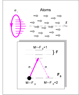
Figure 2: Schematic diagram showing the geometry of the proposed experiment on entanglement between light and atomic subsystems and the scheme of relevant excitation transitions, see text for details.

The processes shown in figures 1 and 2 have practically identical theoretical description. Thus we will discuss them in parallel paying attention to the differences in their physical nature. We begin by introducing the relevant set of the field and atomic variables involved in these processes.

II.2 Field subsystem

The polarization states of the light subsystem can be specified in terms of the following flux-type variables for different Stokes components. The Heisenberg operators for the total photon flux considered at the spatial point $z$ and at the time moment $t$ are given by

$$\hat{\Xi}_{0}(z,t)\;=\;\frac{S_{0}\,c}{2\pi\hbar\,\bar{\omega}}\,\hat{\mathbf{E}}^{(-)}(z,t)\,\hat{\mathbf{E}}^{(+)}(z,t)$$ (1)

where $\hat{\mathbf{E}}^{(\pm)}(z,t)$ are the positive/negative frequency components of the electric field Heiseberg operators. We assume the quasi-monochromatic and forward propagating probe light such that the spectral envelope of the modes has a carrier frequency $\bar{\omega}$, and the light beam has a cross area $S_{0}$.

The Stokes components responsible for three alternative polarization types are given by

$$\hat{\Xi}_{1}(z,t) = \frac{S_{0}\,c}{2\pi\hbar\,\bar{\omega}}\,\left[\hat{E}_{\xi}^{(-)}(z,t)\,\hat{E}_{\xi}^{(+)}(z,t)\right.$$

$$\phantom{\frac{S_{0}\,c}{2\pi\hbar\,\bar{\omega}}\,}\left.-\,\hat{E}_{\eta}^{(-)}(z,t)\,\hat{E}_{\eta}^{(+)}(z,t)\right]$$

$$\hat{\Xi}_{2}(z,t) = \frac{S_{0}\,c}{2\pi\hbar\,\bar{\omega}}\,\left[\hat{E}_{R}^{(-)}(z,t)\,\hat{E}_{R}^{(+)}(z,t)\right.$$

$$\phantom{\frac{S_{0}\,c}{2\pi\hbar\,\bar{\omega}}\,}\left.-\,\hat{E}_{L}^{(-)}(z,t)\,\hat{E}_{L}^{(+)}(z,t)\right]$$

$$\hat{\Xi}_{3}(z,t) = \frac{S_{0}\,c}{2\pi\hbar\,\bar{\omega}}\,\left[\hat{E}_{x}^{(-)}(z,t)\,\hat{E}_{x}^{(+)}(z,t)\right.$$ (2)

$$\phantom{\frac{S_{0}\,c}{2\pi\hbar\,\bar{\omega}}\,}\left.-\,\hat{E}_{y}^{(-)}(z,t)\,\hat{E}_{y}^{(+)}(z,t)\right]$$

These components subsequently define imbalance in the photon fluxes with respect to the $x/y$ Cartesian basis ($\hat{\Xi}_{3}$), to the $\xi/\eta$ Cartesian basis rotated at $\pi/4$-angle ($\hat{\Xi}_{1}$), and to the $R/L$ basis of circular polarizations ($\hat{\Xi}_{2}$), see footnote .

The Stokes variables (2) obey the following commutation relations

$$\left[\hat{\Xi}_{\mathrm{i}}(z,t),\hat{\Xi}_{\mathrm{j}}(z^{\prime},t)\right]\;=\;2i\varepsilon_{\mathrm{i}jk}\,c\,\delta(z-z^{\prime})\hat{\Xi}_{k}(z,t)$$ (3)

where $\varepsilon_{\mathrm{i}jk}=\pm 1$ depending on the order of the indices ${\mathrm{i}}\neq{\mathrm{j}}\neq{\mathrm{k}}$. The $\delta$-function on the right-hand side of this commutation relation is an approximation valid if only a finite bandwidth of the field continuum is important for the correct description of the low frequency fluctuation spectrum. This assumption is in accord with the rotating wave approximation which we will further use in the description of the atom-field interaction. For the processes shown in figures 1 and 2 the commutation relations (3) can be simplified to

$$\left[\hat{\Xi}_{3}(z,t),\hat{\Xi}_{1}(z^{\prime},t)\right]\;=\;2i\,c\,\delta(z-z^{\prime})\bar{\Xi}_{2}$$ (4)

where for the case of small fluctuations the operator on the right-hand side is replaced by its expectation value. This Stokes component is approximately conserved in the linear evolution, and because of the conservation law for the number of photons in the coherent process one has $\bar{\Xi}_{2}=\bar{\Xi}_{0}$. The component $\bar{\Xi}_{0}$ is the integral of motion in our model and $N_{P}=\bar{\Xi}_{0}T$, where $T$ is the interaction time, gives the average number of photons participating in the process.

II.3 Atomic spin subsystem

The angular momentum polarization of $a$-th atom can be conveniently described in the formalism of the irreducible tensor operators

$$\hat{T}_{KQ}^{(a)}=\sqrt{\frac{2K+1}{2F_{0}+1}}\,\sum_{M^{\prime},M}\,C_{F_{0}M\,KQ}^{F_{0}M^{\prime}}\,|F_{0}M^{\prime}\rangle\langle F_{0}M|^{(a)}$$

$$|F_{0}M^{\prime}\rangle\langle F_{0}M|^{(a)}=\sum_{KQ}\,\sqrt{\frac{2K+1}{2F_{0}+1}}\,C_{F_{0}M\,KQ}^{F_{0}M^{\prime}}\,\hat{T}_{KQ}^{(a)}$$

With these expansions the set of atomic dyadic operators originally defined in the subspace of the Zeeman states $|F_{0}M\rangle$, where $F_{0}$ is the total (spin + nuclear) angular momentum of atom and $M$ is its Zeeman projection, is transformed into the set of the relevant irreducible tensor operators. Here $C_{\ldots\,\ldots}^{\ldots}$ are the Clebsh-Gordan coefficients, with the rank and the projection $K,Q$ which respectively vary in the intervals: $0\leq K\leq 2F_{0}$ and $-K\leq Q\leq K$, see Ref.VMK .

The Heisenberg dynamics of the irreducible components (LABEL:2.5) preserves the following commutation relations

$$\left[\hat{T}_{KQ}^{(a)}(t),\hat{T}_{K^{\prime}Q^{\prime}}^{(b)}(t)\right] = \delta_{ab}\,[(2K+1)(2K^{\prime}+1)]^{1/2}\,$$ (9)

$$\times\sum_{K^{\prime\prime}}\;[1-(-1)^{K+K^{\prime}+K^{\prime\prime}}]\,\left\{\begin{array}[]{ccc}K&K^{\prime}&K^{\prime\prime}\\ F_{0}&F_{0}&F_{0}\end{array}\right\}\,$$

$$\times\,(-1)^{2F_{0}+K^{\prime\prime}}\,C^{K^{\prime\prime}Q^{\prime\prime}}_{KQ\,K^{\prime}Q^{\prime}}\,\hat{T}_{K^{\prime\prime}Q^{\prime\prime}}^{(a)}(t)$$

For the interaction processes shown in figures 1 and 2 only the following two combinations of the alignment operators and the longitudinal orientation component contribute to the dynamics of the atomic spin fluctuations

$$\hat{T}_{xy}^{(a)}(t) = \frac{1}{2}\left[\hat{T}_{2-2}^{(a)}(t)\,+\,\hat{T}_{22}^{(a)}(t)\right]$$

$$\hat{T}_{\xi\eta}^{(a)}(t) = -\frac{1}{2i}\left[\hat{T}_{2-2}^{(a)}(t)\,-\,\hat{T}_{22}^{(a)}(t)\right]$$

$$\hat{F}_{z}^{(a)}(t) = \frac{1}{\sqrt{3}}\left[F_{0}(F_{0}+1)(2F_{0}+1)\right]^{1/2}\hat{T}_{10}^{(a)}(t)$$ (10)

where $\hat{F}_{z}^{(a)}(t)$ is the Heisenberg operator of the angular momentum projection for $a$-th atom on $z$-axis. For this set of operators the commutation relation (9) leads

$$\left[\hat{T}_{xy}^{(a)}(t),\hat{T}_{\xi\eta}^{(b)}(t)\right] = \delta_{ab}\,ic_{1}\,\hat{F}_{z}^{(a)}(t)+\delta_{ab}\,ic_{3}\hat{T}_{30}^{(a)}(t)$$

$$\left[\hat{F}_{z}^{(a)}(t),\hat{T}_{xy}^{(b)}(t)\right] = \delta_{ab}\,2i\hat{T}_{\xi\eta}^{(a)}(t)$$

$$\left[\hat{F}_{z}^{(a)}(t),\hat{T}_{\xi\eta}^{(b)}(t)\right] = -\,\delta_{ab}\,2i\hat{T}_{xy}^{(a)}(t)$$ (11)

The coefficients $c_{1}$ and $c_{3}$ are given by

$$c_{1} = \frac{3}{F_{0}(F_{0}+1)(2F_{0}+1)}$$

$$c_{3} = -\frac{6\left[(F_{0}-1)(F_{0}+2)\right]^{1/2}}{\left[7F_{0}(F_{0}+1)(2F_{0}-1)(2F_{0}+1)(2F_{0}+3)\right]^{1/2}}$$

and the higher-rank irreducible component $\hat{T}_{30}$ weighted with coefficient $c_{3}$ contributes only for atoms with $F_{0}>1$.

The operators $\hat{T}_{xy}^{(a)}$ and $\hat{T}_{\xi\eta}^{(a)}$ have clear physical meaning and define the components of alignment tensor with respect to either $x,y$ or $\xi,\eta$ Cartesian frames, which were earlier introduced with definition of the polarization Stokes components of light. These operators can also be related with the transverse components of a quasi-spin, which could be defined in the system of two Zeeman states coupled via the $\Lambda$-type excitation channels shown in figures 1 and 2. However in context of our discussion it is more important to emphasize the tensor nature of these components, which are responsible for the fluctuations of linear birefringence of the sample initiated by either stimulated or spontaneous Raman processes shown in these figures.

The important step in further description of the collective dynamics of the atomic spins consists in assumption that the original discrete distribution of the point-like atomic spins can be smoothed with procedure of the mesoscopic averaging. Then for a mesoscopically thin layer located between $z$ and $z+\Delta z$ one can define

$$\hat{\mathcal{T}}_{xy}(z,t) = \frac{1}{\Delta z}\sum_{z<z_{a}<z+\Delta z}\,\hat{T}_{xy}^{(a)}(t)\,$$

$$\hat{\mathcal{T}}_{\xi\eta}(z,t) = \frac{1}{\Delta z}\sum_{z<z_{a}<z+\Delta z}\,\hat{T}_{\xi\eta}^{(a)}(t)\,$$ (13)

where the sum is extended on the atoms located inside the layer. These expressions define the smoothed spatial distribution of the alignment components for which the first line of commutation relation (11) transforms to

$$\left[\hat{\mathcal{T}}_{xy}(z,t),\hat{\mathcal{T}}_{\xi\eta}(z^{\prime},t)\right]=\delta(z-z^{\prime})\,i\bar{c}_{13}\,\bar{\mathcal{F}}_{z}$$ (14)

$$\bar{c}_{13}=\frac{15}{F_{0}(F_{0}+1)(2F_{0}+1)(2F_{0}+3)}$$

where in the case of small fluctuation the right-hand side is replaced by an expectation value for the density of atomic angular momentum $\bar{\mathcal{F}}_{z}$. As in the previous section we assume that this projection of the collective spin is approximately conserved in the Raman process such that the total angular momentum $F_{\Sigma}=\bar{\mathcal{F}}_{z}L=\pm F_{0}N_{A}$, where $L$ is the sample length and $N_{A}$ is the number of atoms. Since the incoherent losses are ignored $N_{A}$ remains the integral of motion in this model.

II.4 Dynamic equations

The master equation governing the dynamics of atoms-field variables in the Heisenberg picture can be derived similarly to the way it was done in Ref. KMSJP . We apply the effective Hamiltonian derived in that paper and neglect the dissipation channels caused by incoherent scattering.

We will assume that the squeezed probe radiation for the excitation scheme, shown in figure 1, is characterized by a degeneracy parameter (i.e. by a mean number of photons in the coherence volume of the quantum radiation) higher than unity. As was shown in Ref.KSS there is a special scenario when the $\Lambda$-system is probed by extremely weak SPDC light source consisting of strongly correlated photon pairs, which should be cooperatively scattered by all atoms of the ensemble. This process cannot be described by the Hamiltonian of Ref.KMSJP and should be discussed separately.

Omitting the derivation details we present the following Heisenberg wave-type equations describing the temporal and spatial dynamics of the Stokes components and the alignment components

$$\left[\frac{\partial}{\partial z}+\frac{1}{c}\frac{\partial}{\partial t}\right]\hat{\Xi}_{1}(z,t) = \kappa_{1}\,\hat{\Xi}_{3}(z,t)\;-\;2\epsilon\,\bar{\Xi}_{2}\,\hat{\mathcal{T}}_{xy}(z,t)$$

$$\left[\frac{\partial}{\partial z}+\frac{1}{c}\frac{\partial}{\partial t}\right]\hat{\Xi}_{3}(z,t) = -\kappa_{1}\,\hat{\Xi}_{1}(z,t)\;+\;2\epsilon\bar{\Xi}_{2}\hat{\mathcal{T}}_{\xi\eta}(z,t)\,$$

$$\frac{\partial}{\partial t}\hat{\mathcal{T}}_{xy}(z,t) = -\bar{\Omega}\hat{\mathcal{T}}_{\xi\eta}(z,t)\;+\;\bar{c}_{13}\epsilon\,\bar{\mathcal{F}}_{z}\,\hat{\Xi}_{1}(z,t)\,$$

$$\frac{\partial}{\partial t}\hat{\mathcal{T}}_{\xi\eta}(z,t) = \phantom{+}\bar{\Omega}\,\hat{\mathcal{T}}_{xy}(z,t)\;-\;\bar{c}_{13}\epsilon\,\bar{\mathcal{F}}_{z}\,\hat{\Xi}_{3}(z,t)\,$$

These equations are written for the physical obsrevables and have a rather clear physical structure. They show that in a linearized regime the modification of the light and atomic polarization in a forward passage results in a combine action of gyrotropy and linear birefringence. In the discussed case the former manifests itself as an averaged interaction between atoms and light and the latter actually creates the quantum fluctuation interface between these subsystems. Let us point out that in a formal description based on a $\Lambda$-type configuration the fluctuations of birefringence (alignment) components are usually treated as an atomic coherence created by Raman process in a quasi-spin subsystem and the importance of the phase-matching gyrotropy can be underestimated. We show how this effect can be properly taken into consideration by direct solution of Eqs.(LABEL:2.11).

Equations (LABEL:2.11) introduce the following important parameters: $\kappa_{1}$, $\bar{\Omega}=2\Omega_{0}+\Omega_{1}$ and $\epsilon$. The first two describe the changes in the mean classical parameters of light and atoms. $\kappa_{1}$ describes the gyrotropy of the sample caused by the average angular momentum orientation of the atomic spins. $\Omega_{1}$ is the light shift between the Zeeman sublevels $F_{0},M=\pm F_{0}$ and $F_{0},M=\pm F_{0}\mp 2$. It is additionally assumed that the atoms interact with an external magnetic field and $\Omega_{0}$ is the relevant Zeeman splitting for the neighboring sublevels. The third parameter $\epsilon$ is the most important and is responsible for the coupled dynamics of the fluctuations of the polarization components of light and of the atomic alignment components. The microscopic expressions for all these characteristics for the case of hyperfine transitions of alkali atoms are summarized in Appendix A

Before we discuss the solutions of these equations we turn again to the physics of the processes shown in figures 1 and 2. The difference between these processes is only indicated by different signs of $\bar{\mathcal{F}}_{z}$ in the second pair of equations (LABEL:2.11). For positive $\bar{\mathcal{F}}_{z}$ (Fig.1) these equations yield the normal wave-type solution leading to the swapping of the quantum states between the light and spin subsystems. Then the memory protocol can develop in the following way. If the quantum field is prepared in an unknown left-hand polarized squeezed-vacuum state its momentum/position quadrature components can be expressed as

$$X_{P} \propto -ie^{i\theta}a+ie^{-i\theta}a^{\dagger}$$

$$X_{Q} \propto e^{i\theta}a+e^{-i\theta}a^{\dagger}$$ (16)

where the phase $\theta$ determining the orientation of the squeezed and anti-squeezed quadratures in the phase plane as well as their variances are the unknown parameters of the state. If such an unknown squeezed state is superimposed with a classical coherent mode one straightforwardly gets that

$$\hat{\Xi}_{1} \propto X_{P}$$

$$\hat{\Xi}_{3} \propto X_{Q}$$ (17)

The crucial point for the atoms-field dynamics described by equations (LABEL:2.11) and for the memory protocol is that the direction of the axes $x,y$ and $\xi,\eta$ remains completely unknown in the experiment, see figure 1. Thus the unknown squeezed state transforms into the unknown polarization squeezing such that the $\hat{\Xi}_{1}$ component is squeezed and $\hat{\Xi}_{3}$ is anti-squeezed. The dynamics of these components is further developing in accordance with equations (LABEL:2.11) and under certain conditions the squeezed state of light can be converted into the squeezed state of the alignment components of the atomic spin angular momenta.

For the negative sign of $\bar{\mathcal{F}}_{z}$ (Fig.2) there is no normal wave solution of the equations (LABEL:2.11). As we will show in this case there is an exponential enhancement of the quantum fluctuations of the Stokes components and of the atomic alignment. Such an anomalous spin polariton wave describes an entangled state of these subsystems. After interaction the low frequency modes of the polarization and intensity spectrum of the outgoing light will be entangled with the alignment-type standing wave modes of the atomic spins. Such process can be for example utilized in the quantum repeater protocol with remote atomic systems.

III Coupled dynamics of the atomic and field subsystems

The Heisenberg equations (LABEL:2.11) can be solved via the method of Laplace transform similar to how it was done in Ref.KMSJP . The solution and verification of the commutation relations are given in Appendix B. In this section we discuss the physical consequences which are mainly important from the quantum information point of view. For the sake of simplicity and without loss of generality, see Ref.KMSJP , we will ignore the retardation effects and restrict our discussion to the low frequency fluctuations such that in equations (LABEL:2.11) we neglect time derivatives of the field variables. We also restrict our consideration to the special case when the relevant pair of Zeeman sublevels, which is either $|F_{0},F_{0}\rangle$ and $|F_{0},F_{0}-2\rangle$ (Fig.1) or $|F_{0},-F_{0}\rangle$ and $|F_{0},-F_{0}+2\rangle$ (Fig.2), is always degenerate such that $\bar{\Omega}=2\Omega_{0}+\Omega_{1}=0$ during the interaction and $\Omega_{0}=0$ without the interaction. This non-critical but convenient simplification allows us to consider storage of quantum states of light in the time independent standing spin wave without any Zeeman-type oscillations, see appendix B.

The qualitative character of the cooperative dynamics of the atomic and field variables can be illustrated by the dispersion relation (50) for the spin polariton modes and light modes defined in the semi-infinite medium and for infinite interaction time. Then temporal and spatial dynamics of the process can be expressed by the respective Laplace modes $s$ and $p$ introduced by expansion (48). The Laplace variables for the inverse transform can be parameterized as $s=-i\Omega,p=iq$. Then the inverse transform reveals a spectral Fourier expansion over the set of relevant temporal and spatial modes. The wave-type dynamics makes these modes coupled via the following dispersion law

$$\Omega = \frac{A}{q}$$

$$A = -2\bar{c}_{13}\epsilon^{2}\bar{\Xi}_{2}\bar{\mathcal{F}}_{z}$$ (18)

This dispersion relation reflects the coupling of low frequency temporal fluctuations of light to fine scale spatial fluctuations of atoms and of fast temporal fluctuations of light to long scale fluctuations of atoms respectively. For an atomic medium of the length $L$ and a light pulse of the duration $T$, the combination $ATL$, characterizing the overall coupling strength between light pulse and atomic ensemble, quantifies this scale relation in natural units.

III.1 Quantum memory protocol

In the following we apply the input/output relations derived in appendix B to identify the suitable parameters for writing and retrieving to and from a quantum memory. For similar systems the optimization of a quantum memory has been analyzed very thoroughly in the single and few-mode situations GAFSL ; NWRSWWJ , while here we are interested in a multi-mode situation considering pulses of squeezed light of a duration much longer than the inverse bandwidth of squeezing. Prior studies of squeezed state storage in DBP considered a steady state regime, while here we discuss a temporal sequence of writing, storage and retrieval.

III.1.1 Write-in stage

Consider the experimental scheme shown in figure 1 for a pulse-type excitation of the system with a portion of quantum light with the following correlation properties

$$\frac{1}{2}\langle\left\{\hat{\Xi}_{1}(\tau),\hat{\Xi}_{1}(0)\right\}_{+}\rangle = \left(\delta(\tau)+\xi_{1}\,\frac{1}{2\tau_{1}}\,e^{-\frac{|\tau|}{\tau_{1}}}\right)\bar{\Xi}_{2}$$

$$\frac{1}{2}\langle\left\{\hat{\Xi}_{3}(\tau),\hat{\Xi}_{3}(0)\right\}_{+}\rangle = \left(\delta(\tau)+\xi_{3}\,\frac{1}{2\tau_{3}}\,e^{-\frac{|\tau|}{\tau_{3}}}\right)\bar{\Xi}_{2}$$

(19)

where $\{\ldots,\ldots\}_{+}$ denotes the anti-commutator of two observables. These correlation functions describe the output generated by the intra-cavity subthreshold degenerate parametric amplifier, see Ref.GrdCll . The freely propagating light with such correlation properties can be associated with a squeezed state of a harmonic oscillator where $\Xi_{1}$ component is squeezed ($\xi_{1}<0$) and $\Xi_{3}$ component is anti-squeezed ($\xi_{3}>0$) such that $(1+\xi_{1})(1+\xi_{3})=1$. The spectral bandwidth of the informative part of the quantum light is limited by the longest of two correlation times

$$\tau_{1} = \left[\frac{\gamma_{C}}{2}+\kappa_{D}\right]^{-1}$$

$$\tau_{3} = \left[\frac{\gamma_{C}}{2}-\kappa_{D}\right]^{-1}$$ (20)

where $\gamma_{C}$ is the cavity loss rate through the output mirror and $\kappa_{D}$ is the efficiency of the downconversion process. For high level of squeezing one has $\tau_{3}\gg\tau_{1}$. This inequality indicates that the minimal duration $T$ of the quantum light pulse should be considerably longer than the longest time $\tau_{3}\equiv\tau_{c}$.

The general solution (52), given in the appendix B, can be straightforwardly rewritten in the following form

$$\hat{{\mathcal{T}}}_{\mathrm{I}}^{\mathrm{out}}(z)\equiv\cos\kappa_{1}z\,\hat{{\mathcal{T}}}_{xy}(z,T)+\sin\kappa_{1}z\,\hat{{\mathcal{T}}}_{\xi\eta}(z,T)=$$

$$c_{13}\epsilon\bar{\cal F}_{z}\int_{0}^{T}\!dt\,J_{0}\!\left(2[-A(T-t)z]^{1/2}\right)\,\hat{\Xi}_{1}^{\mathrm{in}}(t)+\ldots$$

$$\hat{{\mathcal{T}}}_{\mathrm{I\!I\!I}}^{\mathrm{out}}(z)\equiv\cos\kappa_{1}z\,\hat{{\mathcal{T}}}_{\xi\eta}(z,T)-\sin\kappa_{1}z\,\hat{{\mathcal{T}}}_{xy}(z,T)=$$

$$-c_{13}\epsilon\bar{\cal F}_{z}\int_{0}^{T}\!dt\,J_{0}\!\left(2[-A(T-t)z]^{1/2}\right)\,\hat{\Xi}_{3}^{\mathrm{in}}(t)+\ldots$$

which shows how the input field operators are transferred into space-dependent atomic spin operators. The dots in the right hand side stand for the contributions of the atomic operators responsible for reproduction of input atomic state, which make this transformation imperfect.

The principle condition, which makes the memory protocol feasible, is that for the low-frequency spatial fluctuations on the left hand side of Eqs.(LABEL:3.5) the contribution of the input spin fluctuations on the right hand side is suppressed. In the spectral expansion of the operators $\hat{{\mathcal{T}}}_{\mathrm{I}}^{\mathrm{out}}(z)$ and $\hat{{\mathcal{T}}}_{\mathrm{I\!I\!I}}^{\mathrm{out}}(z)$ such fluctuations belong to the spectral domain $q\lesssim q_{c}=[\frac{|A|T}{L}]^{1/2}$. In accordance with the dispersion law (18), which is asymptotically valid for $T,L\to\infty$, the transform (LABEL:3.5) performs mapping of the field fluctuations within the spectral interval $0<\Omega\lesssim\tau_{c}^{-1}$ onto the spatially dependent spin fluctuations within the spatial spectral domain $\infty>q\gtrsim|A|\tau_{c}$. For reliable mapping of the field quantum state onto the atomic alignment subsystem the latter domain should essentially overlap with the spectral domain where the input spin fluctuations are suppressed. For the efficient memory protocol the following inequalities should be fulfilled

$$|A|\tau_{c} \ll q_{c}=\left[\frac{|A|T}{L}\right]^{1/2}$$

$$L^{-1} \ll q_{c}$$ (22)

These inequalities imply that the contribution of the input spin fluctuations are suppressed and ensure that the spatial fluctuations of $\hat{{\mathcal{T}}}_{\mathrm{I}}^{\mathrm{out}}(z)$ and $\hat{{\mathcal{T}}}_{\mathrm{I\!I\!I}}^{\mathrm{out}}(z)$ correctly reproduce the temporal dynamics of the input field fluctuations (19) in the relevant part of their spectrum. However the dispersion relation (18) has a singular behavior for the function $\Omega=\Omega(q)$ near the point $q\to 0$ such that the shot noise part of the input fluctuation spectrum is reproduced at the zero point of spatial spectrum. Thus near the spectral point $q\to 0$, associated with an integral collective mode of the standing spin waves in the limit $L\to\infty$, the informative part of the fluctuation spectrum will be invisible. However, for the sample with a finite length $L$ the squeezed state can be mapped onto the integral collective modes of $\hat{{\mathcal{T}}}_{\mathrm{I}}^{\mathrm{out}}(z)$ and $\hat{{\mathcal{T}}}_{\mathrm{I\!I\!I}}^{\mathrm{out}}(z)$ if $|A|\tau_{c}\ll L^{-1}\ll q_{c}$ i.e. for a spectrally broad incoming quantum light.

III.1.2 Retrieval stage

For retrieval of the quantum state back onto light the atomic ensemble should be probed with another strong coherent light pulse. Optimal retrieval occurs when

$$\kappa_{1}L=2\pi\times\mathrm{any\ integer}$$ (23)

Then following (51) the output field operators are given by

$$\hat{\Xi}_{1}^{\mathrm{out}}(t)\!\! = \!\!-2\epsilon\bar{\Xi}_{2}^{\prime}\!\int_{0}^{L}\!dz\,J_{0}\!\left(2[-A^{\prime}(L-z)t]^{1/2}\right)\hat{{\mathcal{T}}}_{\mathrm{I}}^{\mathrm{out}}(z)+\ldots$$

$$\hat{\Xi}_{3}^{\mathrm{out}}(t)\!\! = \!\!\phantom{+}2\epsilon\bar{\Xi}_{2}^{\prime}\!\int_{0}^{L}\!dz\,J_{0}\!\left(2[-A^{\prime}(L-z)t]^{1/2}\right)\hat{{\mathcal{T}}}_{\mathrm{I\!I\!I}}^{\mathrm{out}}(z)+\ldots$$

where the initial state of the atoms is $\hat{{\mathcal{T}}}_{\mathrm{I}}^{\mathrm{out}}(z)$ and $\hat{{\mathcal{T}}}_{\mathrm{I\!I\!I}}^{\mathrm{out}}(z)$ modified in the write-in stage of the protocol. The dots on the right hand side again indicate the imperfection of the transform because of the presence of the input field operators associated with the vacuum modes.

The noise contribution caused by the vacuum fluctuation of the input field can be suppressed in the low frequency domain $\Omega<\Omega_{c}^{\prime}=[\frac{|A^{\prime}|L}{T^{\prime}}]^{1/2}$, see Eq.(51). At the retrieval stage of the protocol the spin fluctuations within the spectral interval $0<q\lesssim q_{c}$ are mapped onto the time dependent field fluctuations in the frequency spectral domain $\infty>\Omega\gtrsim|A^{\prime}|l_{c}$, where the correlation length is given by $l_{c}=q_{c}^{-1}\ll L$. At the retrieval stage of the memory protocol the following inequalities should be fulfilled

$$|A^{\prime}|l_{c} \ll \Omega_{c}^{\prime}=\left[\frac{|A^{\prime}|L}{T^{\prime}}\right]^{1/2}$$

$$T^{\prime-1} \ll \Omega_{c}^{\prime}$$ (25)

which, after the obvious replacement of temporal and spatial parameters, are symmetric to the inequalities (22) and have similar physical meaning. Thus the time dynamics of the output field operators $\hat{\Xi}_{1}^{\mathrm{out}}(t)$ and $\hat{\Xi}_{3}^{\mathrm{out}}(t)$ correctly reproduce the spatial distribution of spin fluctuations in the relevant part of the spectrum.

III.1.3 Physical requirements and numerical simulations

Basic requirements for the proposed memory protocol can be summarized by combining the inequalities (22) and (25) where parameters $A$ and $A^{\prime}$ are given by Eq.(18). The following limitation should be imposed on the number of atoms $N_{A}$ and on the numbers of photons in the coherent strong field $N_{P}$ and $N_{P}^{\prime}$ participating in the process at the write-in and retrieval stages respectively

$$\epsilon^{2}N_{A}N_{P} \gg 1$$

$$\epsilon^{2}N_{A}N_{P}^{\prime} \gg 1$$ (26)

The substitution of $l_{c}$ from (22) into (25) yields

$$N_{P}^{\prime}\ll N_{P}$$ (27)

From evaluation of incoherent losses we obtain the following conditions on the numbers of atoms and photons

$$N_{A}\sigma_{F_{0}}^{-} \ll S_{0}$$

$$N_{P}\sigma_{F_{0}-2}^{+},\,N_{P}^{\prime}\sigma_{F_{0}-2}^{+} \ll S_{0}$$ (28)

where $\sigma_{F_{0}}^{-}$ is the cross section of the incoherent scattering for a left-hand polarized light from the atoms populating the Zeeman sublevel $M=F_{0}$ and $\sigma_{F_{0}-2}^{+}$ is the cross section of the incoherent scattering for a right-hand polarized light from the atoms populating the $M=F_{0}-2$ Zeeman sublevel; $S_{0}$ is the beam/sample cross area. The first line indicates that the atomic medium should be transparent for the informative quantum radiation. The second line indicates that the incoherent scattering should have negligible influence on the dynamics of the spin coherence during both the write-in and the retrieval cycles. These requirements lead to the following basic demand on the density of atoms $n_{0}$, resonance radiation wavelength $\lambdabar$ and the sample length $L$: $n_{0}\lambdabar^{2}L\gg 1$, i.e. the on resonance optical depth of the sample needs to be large

Optimization of the inequalities (27) and (28) requires that $N_{P}^{\prime}\leq N_{A}\leq N_{P}$. To explain this choice let us again consider the coherent Raman scattering as the physical background for the memory protocol. In the write-in stage of the protocol the most desirable process is the annihilation of the photons of the quantum modes as a result of the coherent scattering into the classical mode followed by the transfer of their quantum state onto the alignment of atoms. The swapping process can be easier done for the photons in the wings of the spectral distribution (19) and is more difficult to realize for the resonance photons. That is why the process runs more efficiently with a stronger coherent field with $N_{P}\geq N_{A}$. At the retrieval stage the coherent Raman scattering takes photons from the strong mode into the quantum modes. The spin fluctuations of the atomic alignment tensor transfer back into the outgoing modes of the quantum light. To make this process more efficient, i.e. to increase the number of scattering events, it is desirable that the sample is extended and contains a large number of the atoms such that $N_{A}\geq N_{P}^{\prime}$.

In figure 3 we show how the spectral variances of the polarization components of light and atoms are modified after sending the broadband squeezed light ($\tau_{c}\to 0$) through the atomic sample. The graphs clearly display the swapping mechanism at the write-in stage of the memory protocol. The graphs are normalized to the vacuum state variance and the deviations from it are expressed by the respective Mandel parameters $1+\xi_{\mathrm{i}}$ for ${\mathrm{i}}=1,3$, which depend on either frequency $\Omega$ (for light) or wave number $q$ (for atoms). The input squeezed state is described by two spectrally independent parameters $1+\xi_{3}^{\mathrm{in}}=10$ and $1+\xi_{1}^{\mathrm{in}}=0.1$. The suppression of the correlations in the low frequency domain of the temporal spectrum of light is compensated by the enhancement of the correlations in the atoms for the low frequency part of the spatial spectrum. The dominant role of the collective modes in this process is a result of the approximation $\tau_{c}\to 0$.

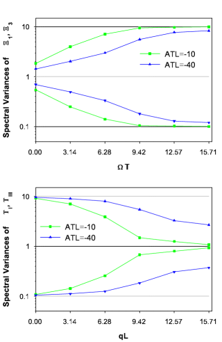
Figure 3: The spectral variances of the Stokes components (upper panel) and of the atomic alignment components (lower panel) before and after the interaction with the broadband squeezed light for cooperative parameter $ATL=-10$ (squares) and $ATL=-40$ (triangles). The black solid lines indicate the original fluctuation spectra in the light and spin subsystems. The gray lines in each of the panels indicate the original spectra for a complementary system.

The data, presented in these graphs, corresponds to the red detuning of light near the $D_{1}$-line of ⁸⁷Rb for atoms in the hyperfine level $F_{0}=1$ and for two selected values of the cooperative interaction parameter $ATL=-10,-40$. The first value corresponds to the detuning $-205\,$MHz from $F_{0}=1\to F=1$ resonance, where $\kappa_{1}=0$ (no gyrotropy effect) and for approximately ten percent losses estimated from Eqs.(28). The second number is achievable for the detuning of a few thousand MHz in the red wing of the $F_{0}=1\to F=1$ transition and for the same level of losses.

Figure 4 shows the spectral variances of the polarization components for the atoms and light at the retrieval stage of the protocol. The figure shows how well the recovered state can reproduce the input. The parameters are chosen such that $A^{\prime}T^{\prime}L=-2$ corresponding to $ATL=-10$ and $A^{\prime}T^{\prime}L=-8$ corresponding to $ATL=-40$. Let us point out once more that for the best overall efficiency, the number of photons in the strong coherent pulse at the retrieval stage should be smaller than the number of photons applied at the write-in stage of the protocol and smaller than the number of atoms. As follows from these results the retrieved quantum state of light can reproduce the input state only in certain parts of the fluctuation spectrum. Further optimization should allow for identification of the best temporal mode, where the retrieval of the original squeezed state would be optimal.

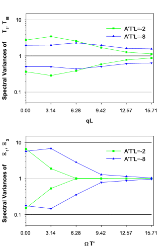
Figure 4: The spectral variances of the alignment components of the atoms (upper panel) and of the retrieved Stokes components of the light (lower panel) after the readout of the state stored in the atoms at the write-in stage of the memory protocol, see Fig.3. The values of cooperative parameter $A^{\prime}T^{\prime}L=-2$ (squares) and $A^{\prime}T^{\prime}L=-8$ (triangles) are coordinated with the data of Fig.3. The black solid lines indicate the original fluctuation spectra in the spin and light subsystems. The gray lines in each of the panels indicate the original spectra for the complementary system.

Figures 5 and 6 show how the spectra of the light and atoms are modified at the write-in and retrieval stages with the finite-bandwidth squeezed light as the input. The dependencies plotted in these graphs illustrate the importance of the dispersion relation between the temporal and spatial modes participating in the protocol. The ratio of the interaction time to the correlation time of the squeezing is taken to be $T/\tau_{c}=10$. As follows from the displayed results, for the finite-bandwidth squeezed light the integral collective modes are not optimal in both storage and retrieval steps of the protocol. A certain optimization procedure is necessary for the best encoding of the quantum information into particular domains and modes of the fluctuation spectra for the light and atoms. Another important observation which follows from these graphs is that the finite bandwidth squeezing is more difficult to store and retrieve than the broadband input state, the fact already established for the storage phase in KMP . This is the direct consequence of the imperfection of the swapping mechanism for mapping the low frequency fluctuations, as follows from the dispersion law discussed above.

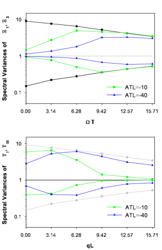
Figure 5: Same as in Fig.3, but for the finite-bandwidth squeezed light. The ratio of interaction time to the correlation time of squeezing for these graphs is $T/\tau_{c}=10$.

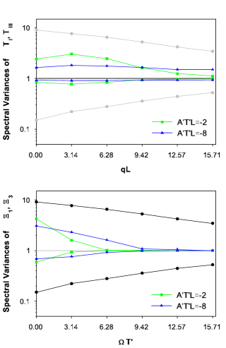
Figure 6: Same as in Fig.4, but for retrieval of the finite-bandwidth squeezed state mapped onto the spin subsystem, see Fig.5. The original spectrum for the squeezed light in the lower panel relates to the case of $T^{\prime}=T$.

III.1.4 Fidelity

Fidelity is the fundamental criterion for any quantum memory or teleportation scenario. It can be relatively simply defined for a single mode situation and for a pure input state, and is more subtle for a general case. In the following we show qualitatively that in the present case the quantum scheme has always a better fidelity than for what can be called a classical memory/measurement protocol.

We assume that the classical memory scheme utilizes a balance homodyne detection of the input squeezed state for the measurement of its parameters. The measurement should yield the degree of squeezing and the directions of the linear polarizations shown in figure 1. Such a procedure is displayed in figure 7a as an overlap of the Wigner function associated with the input state with its measured counterpart. This overlap in the limit of high level of squeezing can be expressed by the following fidelity

$$F\approx\frac{1}{\sqrt{1+(D_{3}\theta_{N}})^{2}}$$ (29)

where $D_{3}=(1+\xi_{3})/2$ is half of the variance for the anti-squeezed $\Xi_{3}$ component, which is assumed to be reliably defined, and $\theta_{N}\sim\pi/N$ is the angular uncertainty remaining after $N$ measuring attempts to identify direction of $x,y$ or $\xi,\eta$ axes. Following Ref.KuprSk the following constraint should be fulfilled in order to make the classical protocol efficient

$$\sqrt{\frac{\tau_{c}}{T_{N}}}<(D_{3}\theta_{N})^{2}<1$$ (30)

where $T_{N}\sim T/N$ is the duration of each measuring attempt as a fraction of the total measuring time $T$. It is clear that for $D_{3}\to\infty$ the number of measurements $N$ should grow up to infinity such that for any limited time $T$ the constraint (30) can never be fulfilled.

On the contrary, in the quantum memory protocol it is only necessary to effectively reproduce the variances associated with the squeezed and anti-squeezed polarization components. The directions of the $x,y$ and $\xi,\eta$ axes remain completely unknown in the interaction process. This is shown in figure 7b with a more effective overlap than in case of figure 7a. The fidelity can be conveniently written in terms of Mandel parameter for the input and output states

$$F=\frac{2}{\left[(2+\xi_{1}^{\mathrm{in}}+\xi_{1}^{\mathrm{out}})(2+\xi_{3}^{\mathrm{in}}+\xi_{3}^{\mathrm{out}})\right]^{1/2}}$$ (31)

where ”out” characteristics should be associated with optimally defined spatial mode. Comparing (29) and (31) for the same ratio $T/\tau_{c}$ and for the high level of squeezing one can expect that in the optimized case the fidelity for the quantum protocol will be always higher than the relevant classical benchmark.

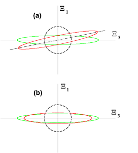
Figure 7: The overlap of the Wigner function for the input squeezed state (green ellipse) with its ”classical” (a) and ”quantum” (b) counterparts (red ellipses).

III.2 Atoms-field entanglement

The entanglement between the light and the atomic alignment subsystems created in the process shown in figure 2 is attained in a result of the transformations (56), (57) under the constraint (23). The entanglement can be written in the following canonic form

$$\int_{0}^{T}h(t)\,\hat{\Xi}_{1}^{\mathrm{out}}(t)\,dt-\int_{0}^{L}g(z)\,\hat{{\mathcal{T}}}_{\mathrm{I}}^{\mathrm{out}}(z)\,dz \to 0$$

$$\int_{0}^{T}h(t)\,\hat{\Xi}_{3}^{\mathrm{out}}(t)\,dt+\int_{0}^{L}g(z)\,\hat{{\mathcal{T}}}_{\mathrm{I\!I\!I}}^{\mathrm{out}}(z)\,dz \to 0\phantom{3.13}$$ (32)

The alignment spin waves $\hat{{\mathcal{T}}}_{\mathrm{I}}^{\mathrm{out}}(z)$ and $\hat{{\mathcal{T}}}_{\mathrm{I\!I\!I}}^{\mathrm{out}}(z)$ are defined by the upper lines of Eqs.(LABEL:3.5). The standard entanglement between the quadrature components of certain collective field and atomic spin modes can be recognized in Eqs.(32) , see also relations (16) and (17).

Formally the temporal mode $h(t)$ and the spatial mode $g(z)$ can be found by solving the following integral equations

$$h(t)+\int_{t}^{T}dt^{\prime}\,\left[\frac{AL}{t^{\prime}-t}\right]^{1/2}I_{1}\left(2\left[AL(t^{\prime}-t)\right]^{1/2}\right)\,h(t^{\prime})$$

$$-\bar{c}_{13}\epsilon\bar{\mathcal{F}}_{z}\int_{0}^{L}dz\,I_{0}\left(2\left[A(T-t)z\right]^{1/2}\right)\,g(z)\to 0\phantom{(3...14)}$$

$$g(z)+\int_{z}^{L}dz^{\prime}\,\left[\frac{AT}{z^{\prime}-z}\right]^{1/2}I_{1}\left(2\left[AT(z^{\prime}-z)\right]^{1/2}\right)\,g(z^{\prime})$$

$$+2\epsilon\bar{\Xi}_{2}\int_{0}^{T}dt\,I_{0}\left(2\left[A(L-z)t\right]^{1/2}\right)\,h(t)\to 0\phantom{(3...14)}$$ (33)

Due to the presence of non-symmetric integral operators in the upper lines of these equations their actual solution does not responsibly exist in terms of real functions. One can search for a pair of real functions $h(t)$ and $g(z)$ which minimize the absolute value of the left hand side of (33). This circumstance is reflected by the ”limit to zero” in the right hand side, which can be approximately approached for certain optimal observation conditions.

It is intuitively clear that this can be achieved for a system consisting of a large number of atoms ($\epsilon|\bar{\mathcal{F}}_{z}|L\gg 1$) and of a large number of coherent photons ($\epsilon\bar{\Xi}_{2}T\gg 1$). Using the common properties of the Fredholm-type equations the solutions for the spatial and temporal modes of (32) can be found in terms of the eigenfunctions of the integral equations (33).

IV Conclusion

We discuss the polarization sensitive interaction between the Stokes components of light and the alignment components of the atomic ensemble as a resource for quantum information interface. Our model accurately describes the quantum nature of interaction between the spin subsystem of ultracold alkali atoms and a plain light wave propagating through the sample, in the absence of losses. The method has two important advantages. First, the process does not require any special manipulations like a feedback or adjustment of the driving classical light. This creates good outlooks for its experimental implementation. Second, the model yields an analytical solution under rather general assumptions. This allows for a convenient and clear interpretation of the Heisenberg dynamics of atoms and field at every step of the discussed quantum information protocols.

We consider two basic protocols: quantum memory and quantum entanglement. The memory protocol is an example of the swapping mechanism between the atomic and field subsystems. The quantum information, which is originally encoded in the polarization degrees of freedom of the light wave, can be mapped onto the spin standing wave associated with atomic alignment components. However because of the multimode nature of the interaction process the quantum information can be spread among a number of spatial spectral modes. We show how the protocol, particularly at the final retrieval stage, can be optimized. As an important step of such optimization we have comprehensively discussed the imperfection of the quantum memory channel and made qualitative comparison of its figure of merit with a competing classical memory/measurement scheme.

The second protocol is generation of entanglement in the spin oriented atomic ensemble probed with a circularly polarized coherent light mode. Forward scattered Raman photons appear strongly correlated with an alignment-type coherence of atomic scatterers. When the process becomes extended in space as well as in time it creates pairs of entangled temporal and spatial modes. We introduced the system of two integral equations, whose solution defines the structure of these modes.

Appendix A Coupling parameters of the Heisenberg equations

The wave-type Heisenberg equations (LABEL:2.11) straightforwardly follow from the commutation relations between the operators of the respective quantum observables with an effective Hamiltonian responsible for the process of coherent forward scattering. The latter was derived in Ref.KMSJP . The exact equations are linearized with assumption of small fluctuations when $\bar{\Xi}_{2}$ and $\bar{\mathcal{F}}_{z}$ are approximately conserved and interpreted as classical values. Then the gyrotropy constant is given by

$$\kappa_{1}=\sum_{F}\bar{\alpha}_{F_{0}F}^{(1)}(\bar{\omega})\frac{\sqrt{3}\,\bar{\mathcal{F}}_{z}}{\left[F_{0}(F_{0}+1)(2F_{0}+1)\right]^{1/2}}$$ (34)

Here $\bar{\alpha}_{F_{0}F}^{(1)}(\bar{\omega})$ is the dimensionless orientation income into the polarizability tensor for the $F_{0}\to F$ hyperfine transition

$$\bar{\alpha}_{F_{0}F}^{(1)}(\bar{\omega}) = (-1)^{F+F_{0}}\frac{1}{\sqrt{2}}\,\left\{\begin{array}[]{ccc}1&1&1\\ F_{0}&F_{0}&F\end{array}\right\}\,$$ (38)

$$\times\frac{4\pi\bar{\omega}}{S_{0}\,c}\,\frac{|d_{F_{0}F}|^{2}}{-\hbar(\bar{\omega}-\omega_{FF_{0}})}$$

where $d_{F_{0}F}$ is the reduced dipole moment and $\omega_{FF_{0}}$ is the transition frequency. The light shift is given by

$$\Omega_{1}=\sum_{F}\bar{\alpha}_{F_{0}F}^{(1)}(\bar{\omega})\frac{\sqrt{3}\,\bar{\Xi}_{2}}{\left[F_{0}(F_{0}+1)(2F_{0}+1)\right]^{1/2}}$$ (39)

This expression is similar to definition of the gyrotropy constant (34) because both the parameters come from the same Faraday-type interaction term of the effective Hamiltonian.

The coupling constant $\epsilon$ responsible for the alignment-type interaction is given by

$$\epsilon=\frac{1}{2}\sum_{F}\bar{\alpha}_{F_{0}F}^{(2)}(\bar{\omega})$$ (40)

where $\bar{\alpha}_{F_{0}F}^{(2)}(\bar{\omega})$ is the dimensionless alignment contribution into the polarizability tensor

$$\bar{\alpha}_{F_{0}F}^{(2)}(\bar{\omega}) = (-1)^{1+F+F_{0}}\left\{\begin{array}[]{ccc}1&1&2\\ F_{0}&F_{0}&F\end{array}\right\}\,$$ (44)

$$\times\frac{4\pi\bar{\omega}}{S_{0}\,c}\,\frac{|d_{F_{0}F}|^{2}}{-\hbar(\bar{\omega}-\omega_{FF_{0}})}$$

All the parameters are the spectrally dependent values such that $\kappa_{1}=\kappa_{1}({\bar{\omega}})$, $\Omega_{1}=\Omega_{1}({\bar{\omega}})$, $\epsilon=\epsilon({\bar{\omega}})$ and this dependence can be very important in practical calculations.

Appendix B The solution of the Heisenberg equations

We derive the solution for those physical conditions when only low frequency temporal fluctuations are considered as a quantum information carrier. That lets us completely ignore the retardation effects associated with a finite sample size. Practically this means that we can neglect the time derivations in the first two lines of the system (LABEL:2.11).

As a first step we make the following local rotational transformations for the Stokes components of the field subsystem

$$\hat{\Xi}_{\mathrm{I}}(z,t) = \cos\varphi(z,t)\,\hat{\Xi}_{1}(z,t)-\sin\varphi(z,t)\,\hat{\Xi}_{3}(z,t)\phantom{(B1)}$$

$$\hat{\Xi}_{\mathrm{I\!I\!I}}(z,t) = \sin\varphi(z,t)\,\hat{\Xi}_{1}(z,t)+\cos\varphi(z,t)\,\hat{\Xi}_{3}(z,t)$$ (45)

and for the alignment components of the atomic subsystem

$$\hat{{\mathcal{T}}}_{\mathrm{I}}(z,t)\!\! = \!\!\cos\varphi(z,t)\hat{{\mathcal{T}}}_{xy}(z,t)+\sin\varphi(z,t)\hat{{\mathcal{T}}}_{\xi\eta}(z,t)\phantom{\ (B.2)}$$

$$\hat{{\mathcal{T}}}_{\mathrm{I\!I\!I}}(z,t)\!\! = \!\!-\sin\varphi(z,t)\hat{{\mathcal{T}}}_{xy}(z,t)+\cos\varphi(z,t)\hat{{\mathcal{T}}}_{\xi\eta}(z,t)$$ (46)

where $\varphi(z,t)=\kappa_{1}z\!+\!\bar{\Omega}t$. Without losing of generality the parameter $\bar{\Omega}$ can be set as $0$ to ignore any non-principle freely precession of atomic spins associated with external magnetic field and light shift. It is also convenient to set the sample length $L$ as $\kappa_{1}L=(2\pi\times\mathrm{any\ integer})$, then the pair of Stokes variables $\hat{\Xi}_{\mathrm{I}}(z,t)$, $\hat{\Xi}_{\mathrm{I\!I\!I}}(z,t)$ and $\hat{\Xi}_{1}(z,t)$, $\hat{\Xi}_{3}(z,t)$ will coincide at the output of the sample.

Applying the orthogonal transformations (45) and (46) to the system (LABEL:2.11) the latter can be rewritten in the following form

$$\frac{\partial}{\partial z}\hat{\Xi}_{\mathrm{I}}(z,t) = -2\epsilon\,\bar{\Xi}_{2}\,\hat{\mathcal{T}}_{\mathrm{I}}(z,t)$$

$$\frac{\partial}{\partial z}\hat{\Xi}_{\mathrm{I\!I\!I}}(z,t) = \phantom{+}2\epsilon\,\bar{\Xi}_{2}\,\hat{\mathcal{T}}_{\mathrm{I\!I\!I}}(z,t)$$

$$\frac{\partial}{\partial t}\hat{\mathcal{T}}_{\mathrm{I}}(z,t) = \phantom{+}\bar{c}_{13}\epsilon\,\bar{\mathcal{F}}_{z}\,\hat{\Xi}_{\mathrm{I}}(z,t)\,$$

$$\frac{\partial}{\partial t}\hat{\mathcal{T}}_{\mathrm{I\!I\!I}}(z,t) = -\bar{c}_{13}\epsilon\,\bar{\mathcal{F}}_{z}\,\hat{\Xi}_{\mathrm{I\!I\!I}}(z,t)\,$$ (47)

Then its solution can be found by the method of Laplace transform.

To show this we can define the Laplace images of the space-time dependent Stokes components of the probe light and of the collective alignment components of atoms

$$\hat{\Xi}_{\mathrm{i}}(p,s) = \int_{0}^{\infty}\int_{0}^{\infty}\!dz\,dt\,e^{-pz-st}\,\hat{\Xi}_{\mathrm{i}}(z,t)$$

$$\hat{{\mathcal{T}}}_{\mu}(p,s) = \int_{0}^{\infty}\int_{0}^{\infty}\!dz\,dt\,e^{-pz-st}\,\hat{{\mathcal{T}}}_{\mu}(z,t)$$ (48)

with ${\mathrm{i}}=\mathrm{I,I\!I\!I}$ and $\mu=\mathrm{I,I\!I\!I}$. Then equations (47) is transformed to the system of algebraic equations, which in turn can be straightforwardly solved similar to how it was done in Appendix C of Ref.KMSJP . The important parameter for this procedure is the determinant of the system, which is given by

$$\Delta(p,s)\;=\;\left[sp+2\bar{c}_{13}\epsilon^{2}\bar{\Xi}_{2}\bar{\mathcal{F}}_{z}\right]^{2}$$ (49)

and its pole

$$s = \frac{A}{p}$$ (50)

with $A=-2\bar{c}_{13}\epsilon^{2}\bar{\Xi}_{2}\bar{\mathcal{F}}_{z}$, can be linked with the dispersion law for the spin polariton wave propagating through the sample, see Eq.(18) and discussion around it.

Finally for $A<0$ one obtains the following solution for the Stokes components of the light subsystem

$$\hat{\Xi}_{\mathrm{I}}(L,t) = \hat{\Xi}_{\mathrm{I}}^{\mathrm{in}}(t)-\int_{0}^{t}\!dt^{\prime}\left[\frac{-AL}{t-t^{\prime}}\right]^{1/2}J_{1}\left(2\left[-AL(t-t^{\prime})\right]^{1/2}\right)\hat{\Xi}_{\mathrm{I}}^{\mathrm{in}}(t^{\prime})$$

$$-2\epsilon\bar{\Xi}_{2}\int_{0}^{L}\!dz\,J_{0}\left(2\left[-A(L-z)t\right]^{1/2}\right)\hat{{\mathcal{T}}}_{\mathrm{I}}^{\mathrm{in}}(z)$$

$$\hat{\Xi}_{\mathrm{I\!I\!I}}(L,t) = \hat{\Xi}_{\mathrm{I\!I\!I}}^{\mathrm{in}}(t)-\int_{0}^{t}\!dt^{\prime}\left[\frac{-AL}{t-t^{\prime}}\right]^{1/2}J_{1}\left(2\left[-AL(t-t^{\prime})\right]^{1/2}\right)\hat{\Xi}_{\mathrm{I\!I\!I}}^{\mathrm{in}}(t^{\prime})$$ (51)

$$+2\epsilon\bar{\Xi}_{2}\int_{0}^{L}\!dz\,J_{0}\left(2\left[-A(L-z)t\right]^{1/2}\right)\hat{{\mathcal{T}}}_{\mathrm{I\!I\!I}}^{\mathrm{in}}(z)$$

and for the alignment components of the spin subsystem

$$\hat{\mathcal{T}}_{\mathrm{I}}(z,T) = \hat{\mathcal{T}}_{\mathrm{I}}^{\mathrm{in}}(z)-\int_{0}^{z}\!dz^{\prime}\left[\frac{-AT}{z-z^{\prime}}\right]^{1/2}J_{1}\left(2\left[-AT(z-z^{\prime})\right]^{1/2}\right)\hat{\mathcal{T}}_{\mathrm{I}}^{\mathrm{in}}(z^{\prime})$$

$$+\bar{c}_{13}\epsilon\bar{\mathcal{F}}_{z}\int_{0}^{T}\!dt\,J_{0}\left(2\left[-A(T-t)z\right]^{1/2}\right)\hat{\Xi}_{\mathrm{I}}^{\mathrm{in}}(t)$$

$$\hat{\mathcal{T}}_{\mathrm{I\!I\!I}}(z,T) = \hat{\mathcal{T}}_{\mathrm{I\!I\!I}}^{\mathrm{in}}(z)-\int_{0}^{z}\!dz^{\prime}\left[\frac{-AT}{z-z^{\prime}}\right]^{1/2}J_{1}\left(2\left[-AT(z-z^{\prime})\right]^{1/2}\right)\hat{\mathcal{T}}_{\mathrm{I\!I\!I}}^{\mathrm{in}}(z^{\prime})$$ (52)

$$-\bar{c}_{13}\epsilon\bar{\mathcal{F}}_{z}\int_{0}^{T}\!dt\,J_{0}\left(2\left[-A(T-t)z\right]^{1/2}\right)\hat{\Xi}_{\mathrm{I\!I\!I}}^{\mathrm{in}}(t)$$

Here $L$ is the sample length and $T$ is the interaction time. The solution performs an integral transform of the Heisenberg operators for the Stokes components in the incident light $\hat{\Xi}_{\mathrm{i}}^{\mathrm{in}}(t)$ and of initial Schrödinger operators for the alignment components of atomic spins $\hat{\mathcal{T}}_{\mu}^{\mathrm{in}}(z)$. The kernels of the transform are expressed by the cylindrical Bessel functions of the zeroth $J_{0}(\ldots)$ and first $J_{1}(\ldots)$ order. The original form of atomic and field operators can be recovered with the orthogonal transformations reverse to (45) and (46).

The derived solution preserves the following commutation relations

$$\left[\hat{\Xi}_{\mathrm{I\!I\!I}}(z,t),\hat{\Xi}_{\mathrm{I}}(z,t^{\prime})\right] = 2i\,\delta(t-t^{\prime})\bar{\Xi}_{2}$$

$$\left[\hat{\mathcal{T}}_{\mathrm{I\!I\!I}}(z,t),\hat{\mathcal{T}}_{\mathrm{I}}(z^{\prime},t)\right] = -i\bar{c}_{13}\,\delta(z-z^{\prime})\,\bar{\mathcal{F}}_{z}$$ (53)

The commutation relation for the Stokes components, given by the first line, differs from the original commutation relation in form (4). That is direct consequence of our ignoring the retardation effects. The argument of $\delta$-function, which generally is $t-t^{\prime}-(z-z^{\prime})/c$, can be only approximately reproduced in the assumptions we did. The solution also obeys the following important cross-type commutation relations between the field and atomic variables

$$\left[\hat{\Xi}_{\mathrm{i}}(z,t),\hat{\mathcal{T}}_{\mu}(z^{\prime},t^{\prime})\right]=-2i\bar{c}_{13}\epsilon\,g_{{\mathrm{i}}\mu}\bar{\Xi}_{2}\bar{\mathcal{F}}_{z}$$

$$\times J_{0}\left(2\left[-A(z-z^{\prime})(t-t^{\prime})\right]^{1/2}\right)\left[\theta(t-t^{\prime})-\theta(z^{\prime}-z)\right]$$

where the matrix $g_{{\mathrm{i}}\mu}$ (with ${\mathrm{i}},\mu=\mathrm{I,I\!I\!I}$) is given by

$$g_{{\mathrm{i}}\mu}=\left(\begin{array}[]{cc}0,&1\\ 1,&0\end{array}\right)$$ (55)

These commutation relations clear indicate that the atomic and field variables always commute before and after interaction.

For $A>0$ one obtains the following solution for the Stokes components of the light subsystem

$$\hat{\Xi}_{\mathrm{I}}(L,t) = \hat{\Xi}_{\mathrm{I}}^{\mathrm{in}}(t)+\int_{0}^{t}\!dt^{\prime}\left[\frac{AL}{t-t^{\prime}}\right]^{1/2}I_{1}\left(2\left[AL(t-t^{\prime})\right]^{1/2}\right)\hat{\Xi}_{\mathrm{I}}^{\mathrm{in}}(t^{\prime})$$

$$-2\epsilon\bar{\Xi}_{2}\int_{0}^{L}\!dz\,I_{0}\left(2\left[A(L-z)t\right]^{1/2}\right)\hat{{\mathcal{T}}}_{\mathrm{I}}^{\mathrm{in}}(z)$$

$$\hat{\Xi}_{\mathrm{I\!I\!I}}(L,t) = \hat{\Xi}_{\mathrm{I\!I\!I}}^{\mathrm{in}}(t)+\int_{0}^{t}\!dt^{\prime}\left[\frac{AL}{t-t^{\prime}}\right]^{1/2}I_{1}\left(2\left[AL(t-t^{\prime})\right]^{1/2}\right)\hat{\Xi}_{\mathrm{I\!I\!I}}^{\mathrm{in}}(t^{\prime})$$ (56)

$$+2\epsilon\bar{\Xi}_{2}\int_{0}^{L}\!dz\,I_{0}\left(2\left[A(L-z)t\right]^{1/2}\right)\hat{{\mathcal{T}}}_{\mathrm{I\!I\!I}}^{\mathrm{in}}(z)$$

and for the alignment components of the spin subsystem

$$\hat{\mathcal{T}}_{\mathrm{I}}(z,T) = \hat{\mathcal{T}}_{\mathrm{I}}^{\mathrm{in}}(z)+\int_{0}^{z}\!dz^{\prime}\left[\frac{AT}{z-z^{\prime}}\right]^{1/2}I_{1}\left(2\left[AT(z-z^{\prime})\right]^{1/2}\right)\hat{\mathcal{T}}_{\mathrm{I}}^{\mathrm{in}}(z^{\prime})$$

$$+\bar{c}_{13}\epsilon\bar{\mathcal{F}}_{z}\int_{0}^{T}\!dt\,I_{0}\left(2\left[A(T-t)z\right]^{1/2}\right)\hat{\Xi}_{\mathrm{I}}^{\mathrm{in}}(t)$$

$$\hat{\mathcal{T}}_{\mathrm{I\!I\!I}}(z,T) = \hat{\mathcal{T}}_{\mathrm{I\!I\!I}}^{\mathrm{in}}(z)+\int_{0}^{z}\!dz^{\prime}\left[\frac{AT}{z-z^{\prime}}\right]^{1/2}I_{1}\left(2\left[AT(z-z^{\prime})\right]^{1/2}\right)\hat{\mathcal{T}}_{\mathrm{I\!I\!I}}^{\mathrm{in}}(z^{\prime})$$ (57)

$$-\bar{c}_{13}\epsilon\bar{\mathcal{F}}_{z}\int_{0}^{T}\!dt\,I_{0}\left(2\left[A(T-t)z\right]^{1/2}\right)\hat{\Xi}_{\mathrm{I\!I\!I}}^{\mathrm{in}}(t)$$

Here the functions $I_{0}(\ldots)$ and $I_{1}(\ldots)$ are the modified Bessel functions of the zeroth and first order. The solution obeys the commutation relations (53) and the cross-type commutation relations are now given by

$$\left[\hat{\Xi}_{\mathrm{i}}(z,t),\hat{\mathcal{T}}_{\mu}(z^{\prime},t^{\prime})\right]=-2i\bar{c}_{13}\epsilon\,g_{{\mathrm{i}}\mu}\bar{\Xi}_{2}\bar{\mathcal{F}}_{z}$$

$$\times I_{0}\left(2\left[A(z-z^{\prime})(t-t^{\prime})\right]^{1/2}\right)\left[\theta(t-t^{\prime})-\theta(z^{\prime}-z)\right]$$

References

- (1) Samuel L. Braunstein and Peter van Loock, Quantum information with continuous variables, Rev. Mod. Phys. 77, 513 (2005).
- (2) T.C. Ralph, Quantum optical systems for implementation of quantum information processing, Rep. Prog. Phys. 69, 853 (2006)
- (3) A.E. Kozhekin, K. Mølmer, E.S. Polzik, Phys. Rev. A62, 033809 (2000).
- (4) J. Sherson, B. Julsgaard, and E.S. Polzik. Advances of Atomic Molecular and Optical Physics, November 2006.
- (5) K. Hammerer, K. Mølmer, E.S. Polzik, J.I. Cirac. Phys. Rev. A70, 044304 (2004); J. Sherson, J. Fiurasek, K. Mølmer, A. Sørensen, and E.S. Polzik. Phys. Rev. A74, 011802 (2006); C.A. Muschick, K. Hammerer, E.S. Polzik, J.I. Cirac, Phys. Rev. A73 062329 (2006).
- (6) M. Fleischhauer and M.D. Lukin, Phys. Rev. Lett. 84, 5094, (2000).
- (7) A.V. Gorshkov, A. André, M. Fleischhauer, A.S. Sørensen, M.D. Lukin, quant-ph/0604037v1.
- (8) B. Julsgaard, J. Sherson, J. Fiurasek, J.I. Cirac, and E.S. Polzik, Experimental demonstration of quantum memory for light, Nature 432, 482 (2004).
- (9) K. Hammerer, I. Cirac, E.S. Polsik. Phys. Rev. A72 052313 (2005); J. Sherson, H. Krauter, R.K. Olsson, B. Julsgaard, K. Hammerer, I. Cirac, E.S. Polsik. Nature 443 557-560 (2006).
- (10) M.D. Eisaman, A. André, F. Massou, M. Fleishhauer, A.S. Zibrov, M.D. Lukin, Nature 438, 837 (2005); T. Chanilière, D.N. Matsukevich, S.D. Jenkins, S.Y. Lan, T.A.B. Kennedy, A. Kuzmich, Nature 438, 833 (2005)
- (11) J. Laurat, H. de Riedmatten, D. Felinto, C.W. Chou, E.W. Schomburg, H.J. Kimble, Optics Express 14, 6912-6918 (2006).
- (12) M.G. Raymer, J. Mostowski, Phys. Rev. A24, 1980 (1981); M.G. Raymer, I.A. Walmsley, J. Mostowski, B. Sobolevska A32, 332 (1985).
- (13) A. Dantan, A. Bramati, M. Pinard, Phys. Rev. A71, 043801 (2005).
- (14) W. Wasilevski, M.G. Raymer, Phys. Rev. A73, 063816 (2006).
- (15) J. Nunn, I.A. Walmsley, M.G. Raymer, K. Surmacz, F.C. Waldermann, Z. Wang, D. Jaksch, quant-ph/0603268 (2006).
- (16) D.V. Kupriyanov, O.S. Mishina, I.M. Sokolov, B. Julsgaard, E.S. Polzik, Phys. Rev. A77, 032348 (2005).
- (17) O.S. Mishina, D.V. Kupriyanov, E.S. Polzik, Proceedings of the NATO Advanced Research Workshop, Crete 2005 Quantum information processing from theory to experiment, 199, 346-352 (2006), quant-ph/0509220.
- (18) D. Gottesman, J. Preskill, Phys. Rev. A63, 022309 (2001).
- (19) This definition yields the expansion of the polarization tensor in the projector algebra of Pauli matrices with respect to the basis of linear polarizations, see L.D. Landau E.M. Lifshits The Classical Theory of Fields (Pergamon Press, London, 1951). In literature it is often used an alternative definition with expansion over the Pauli matrices with respect to the basis of circular polarizations.
- (20) D.A. Varshalovich, A.N. Maskalev, V.K. Khersonskii, Quantum Theory of Angular Momentum (World Scientific Singapore, 1988).
- (21) D.V. Kupriyanov, I.M. Sokolov, A.V. Slavgorodskii, Phys. Rev. A68, 043815, (2003).
- (22) M.J. Collett, C.W. Gardiner, Phys. Rev. A30, 1386 (1984).
- (23) D.V. Kupriyanov, I.M. Sokolov, Sov. Phys. JETP 83, 460 (1996).