Abstract

We study the threshold conditions of spatial self organization combined with collective coherent optical backscattering of a thermal gaseous beam moving in a high Q ring cavity with counter propagating pump. We restrict ourselves to the limit of large detuning between the particles optical resonances and the light field, where spontaneous emission is negligible and the particles can be treated as polarizable point masses. Using a linear stability analysis in the accelerated rest frame of the particles we derive an analytic bounds for the selforganization as a function of particle number, average velocity, temperature and resonator parameters. We check our results by a numerical iteration procedure as well as by direct simulations of the N-particle dynamics. Due to momentum conservation the backscattered intensity determines the average force on the cloud, which gives the conditions for stopping and cooling a fast molecular beam.

OCIS codes: (000.0000) General.

1 Introduction

Light forces have become an essential tool to cool, trap and manipulate atomic gases[1]. Ultimately it allowed to reach BEC and thus the lowest temperatures experimentally available[2]. Ever since this success there has been an ongoing quest to extend laser cooling to more atomic species and also molecules. Here the need for a closed optical cycling transition and the preparation of an initial sample of sufficient low temperature and high phase space density to start the cooling process has posed severe limitations. In particular for molecules, spontaneous emission induced by the laser fields populates a great manifold of electronic and rovibrational levels, which hampers the standard laser cooling techniques.

Recently is has been theoretically predicted[3, 4, 5] and experimentally confirmed [6, 7, 8] that using high Q resonators for the cooling light fields, the role of spontaneous emission can be strongly suppressed in laser cooling. As one further decisive experiment superradiant enhancement of cavity cooling was recently demonstrated for Cesium atoms in a confocal cavity[9]. Although the experiments were performed on atoms, this opens very promising prospects on molecules as well. Trapping and cooling of atoms in a far detuned ring cavity field was recently also achieved[10, 11, 27].

As most sources of gaseous cold molecules are fast beams, the second problem to be dealt with is stopping the molecules of such a beam in a very short distance within the vacuum chamber and trap them. A first success in this direction was achieved by using periodic electrostatic fields to stop a molecular beam[12] or by creating the molecules already cold by laser ablation or directly from an atomic magneto optical trap[13].  Here we study the prospects of using a ring cavity setup as an alternative way to slow down a gaseous beam. The particles kinetic energy is converted into light energy using inelastic coherent backscattering. Such a setup, called correlated atomic recoil laser (CARL), was historically proposed in analogy to the Free electron laser (FEL) as laser gain medium using atoms[14, 15]. Many theoretical investigations of these phenomenon, sometimes also called recoil induced resonance (RIR), produced partly controversial results and interpretations [16, 28]. For quite some time experimental efforts to observe clear signatures of CARL were only partly successful[17].

Only recently, a first unambiguous observation of the (inverse-) CARL mechanism to accelerate a cold gas by coherent light scattering in a cavity was achieved in Tübingen using Cesium atoms[18, 26]. These results are in very good agreement with predictions from microscopic dynamic models[19] as well as collective macroscopic descriptions of atoms in ring cavities[20]. Even stronger stopping forces were observed and extrapolated by Vuletić in a standing wave cavity setup[9, 21], where a special bistable atomic selforganization process superradiantly enhances the light forces[3, 23]. In all of the experiments the particles were atoms with a closed optical cycle, which were cold and relatively slow from the start. Nevertheless these results show that the method has great promise.

Here we investigate the experimental conditions necessary to stop and trap a fast molecular beam by help of a single side pumped ring cavity geometry. The idea relates closely to the original idea of CARL, but we are interested in stopping and cooling particles and not in laser gain. In contrast to most previous work we consider the limit of large detuning, where inversion and spontaneous emission from the particles plays no role. This enables one to adiabatically eliminate the excited states from the dynamics, which allows us to apply the results to any point like objects with suitable polarizability and in particular cold molecules.

In this limit the equations simplify dramatically but, of course, the atom field interaction strength per particle gets very small and only cooperative light scattering by a large number of scatters can induce a sufficiently strong force.  In the quasi 1D geometry along the cavity axis this requires a periodic particle arrangement, so that they act like a Bragg mirror coupling the light fields within the resonator. For favorable parameters the interference of the injected and backscattered light creates an optical potential suitable to stabilize such a regular distribution or even induce it via selforganization from an initial flat distribution.

Note that momentum conservation assures that the total force on the cloud is directly related to the backscattered field intensity amounting to two photon momenta per photon decaying from the backward mode. Hence the average force on the gas will always point to the same direction and this acceleration prevents the system from reaching a steady state in the long run. Nevertheless at an intermediate timescale one can expect the atoms to form a transient spatial equilibrium distribution with respect to their accelerated center of mass.

In the following we try to answer two closely related questions in this respect: (1) Under what conditions and circumstances is a homogeneous particle distribution within the resonator unstable against small density fluctuations so that the atoms will start to selforganize? (2) How does the self consistent atom field distribution look like in the regime where self ordering happens and what is the corresponding field intensity and average force on the cloud? As a third important question we address the scaling of the system with particle number, volume and required pump intensity to see whether the effect persists on a macroscopic scale.

Methodically we will adapt an idea already successfully applied to selforganization of atoms in standing wave cavity fields. For this one iteratively determines the self consistent steady state of the cavity field with particles ordered in a way just to create this very same field. The iteration is done assuming fast atomic thermalization and field equilibration but only slow change of the average atomic temperature. In order to adapt the method to particles in a ring cavity we have to change to the accelerated rest frame of the atomic clouds center of mass and additionally assume that the equilibration is faster than the center of mass acceleration. This allows us to find an accelerating position distribution with a largely time independent shape. Investigating the stability and self consistence of this distribution will then give us limiting conditions for which the proposed method should work. In order to check the predictions we then will directly simulate the microscopic equations of motions for finite ensembles of particles and the fields.

2 Model

As model system let us consider a large number $N$ of linearly polarizable point particles interacting with two degenerate counter propagating linearly polarized plane wave ring cavity modes.

The electric field inside the cavity is then

$$\overrightarrow{E}(x,t)=\overrightarrow{E}^{(+)}(x,t)e^{-i\omega_{P}t}+\overrightarrow{E}^{(-)}(x,t)e^{i\omega_{P}t},$$ (1)

$$\overrightarrow{E}^{(+)}(x,t)={\Large\varepsilon}\left[a_{+}(t)e^{ikx}+a_{-}(t)e^{-ikx}\right]\overrightarrow{e}_{z}$$ (2)

$$\overrightarrow{E}^{(-)}=\left[\overrightarrow{E}^{(+)}\right]^{\dagger}$$ (3)

where the electric field per photon is ${\Large\varepsilon}=\sqrt{\hbar\omega_{P}/2\epsilon_{0}V}$ and $a_{\pm}(t)$ gives the field amplitude.

The pump and cavity frequency are assumed to be sufficiently detuned from any optical resonance so that the particles are only weakly excited and the polarization can be adiabatically eliminated. Thus they experience a Stark shift linear in the local intensity and act like a dynamic refractive index in the field. Let the parameter $U_{0}$ denote the light shift per photon in the field. From energy conservation one sees that $U_{0}$ then also has to give the frequency shift of the cavity mode resonances per atom. In terms of the two level linewidth $\Gamma$, detuning $\Delta_{a}$ and atom-field coupling $g$ the effective mode frequency shift reads:

$$U_{0}=\frac{\Delta_{a}}{\Gamma^{2}+\Delta_{a}^{2}}g^{2}.$$ (4)

In a typical setup one sends the molecular beam at average velocity $v_{0}$ into the ringcavity nearly antiparallel to the driven circulating field. The molecules might be moving quite fast (up to ~100 m/s) without some pre-slowing so that the ratio of the Doppler shift to the linewidth $kv/\kappa,$ can be larger than unity but not too large. At much larger velocities, the pump and or the backscattered fields are far of resonance, which requires stronger and stronger pump amplitudes to generate a noticeable force.

In the following we will shift our reference frame to coincide with the particles center of mass motion. Hence, while a particle at rest in the cavity would see a single cavity detuning $\Delta_{c},$ the molecular beam experiences two different Doppler shifted cavity fields with detunings $\Delta_{\pm}=\Delta_{c}\pm kv.$ Thus the equation of motions for the field mode amplitudes are[19]:

$$\frac{d}{dt}a_{\pm}(t)=\left[i\Delta_{\pm}-iNU_{0}-\kappa\right]a_{\pm}(t)-iNU_{0}\left\langle e^{\mp 2ikx}\right\rangle a_{\mp}(t)+\eta_{\pm}.$$ (5)

Here $N$ denotes the particle number and $\eta_{\pm}$ gives the cavity pump amplitudes.  We see that the particles density distribution couples the two counter propagating modes via the spatial average $R_{\pm}=\left\langle e^{\mp 2ikx}\right\rangle$, which is called particle bunching parameter and one has $R_{+}=R_{-}^{\ast}.$ A uniform distribution gives $R_{\pm}\approx 0$, while an optimally ordered phase gives $\left|R_{\pm}\right|\rightarrow 1.$

As second part in our model we include the force of the light field on the particles. Again assuming the large detuning limit this force is dominated by the dipole force[19]. This force can be derived from the effective optical potential, which is determined by the local field intensity simply by:

$${\Large\varepsilon}^{2}V(x)=U_{0}\left|E(x)\right|^{2}.$$ (6)

For $U_{0}<0$, i.e. $\Delta_{a}<0$, this attracts atoms to maxima of the cavity field. Using the definition of the field in terms of the amplitudes $a_{\pm},$ $E^{+}(x)={\Large\varepsilon}(a_{+}e^{ikx}+a_{-}e^{-ikx})$ we get:

$$\left|E{(}x{)}\right|^{2} ={\Large\varepsilon}^{2}\left[\left|a{{}_{+}}\right|^{2}+\left|a{{}_{-}}\right|^{2}+a_{+}a_{-}^{\ast}e^{2ikx}+(a_{+}a_{-}^{\ast})^{\ast}e^{-2ikx}\right]$$ (7)

$$={\Large\varepsilon}^{2}\left[\left|a{{}_{+}}\right|^{2}+\left|a{{}_{-}}\right|^{2}+2\left|a_{+}a_{-}^{\ast}\right|\cos(2kx+\alpha)\right],$$ (8)

with $\alpha$ being the argument of $a_{+}a_{-}^{\ast}$. Note that for calculating the force the constant terms can be omitted from the potential and the average force then simply reads:

$$f(x)=-U_{0}\nabla\left|E{(}x{)}\right|^{2}=-2\hbar kU_{0}\left|a_{+}a_{-}^{\ast}\right|\sin(2kx+\alpha).$$

This force will then act on the atomic distribution and in general one gets a rather complex coupled atom field dynamics[22]. Note that neglecting spontaneous emission (no radiation pressure force) we get momentum conservation of the cavity field modes and gas. This has the consequence that for single side pumping, for every photon in the counter propagating mode one has transferred a momentum of $2\hbar k$ to the cloud. Hence in steady state the average force is directly proportional to the output intensity of the counter propagating mode and we will always have acceleration in the pump direction.

3 Coupled particle field dynamics

3.1 Quasistationary field

Lets us now get some first qualitative insight in the ongoing dynamics for a thermal cloud in a single side pumped ring cavity ($\eta_{+}=\eta,\eta_{-}=0$). While for an empty cavity the field intensity and thus the optical potential is constant along the axis, the particles will coherently backscatter some light and create a periodic intensity modulation. In a typical experimental setup this field redistribution will happen much faster than the typical time on which the particle distribution evolves. Hence the field will almost instantaneously reflect the momentary particle distribution. As the only relevant quantity of the particle distribution entering the field equations is the parameter $R_{-}=\left\langle e^{2ikx}\right\rangle$, the field amplitudes will relax towards:

$$a_{+} =i\eta\frac{\Delta_{-}-NU_{0}+i\kappa}{{(}\Delta_{+}{-}NU_{0}{+i\kappa)(}\Delta_{-}{-}NU_{0}{+}i\kappa{)-}N^{2}U_{0}^{2}\left|R_{-}\right|{{}^{2}}},$$ (9)

$$\ a_{-} =i\eta\frac{NU_{0}R_{-}}{{(}\Delta_{+}{-}NU_{0}{+i\kappa)(}\Delta_{-}{-}NU_{0}{+}i\kappa{)-}N^{2}U_{0}^{2}\left|R_{-}\right|{{}^{2}}}.$$ (10)

To get some more insight in the physical meaning of $R_{-}$ let us consider the prototype case of a periodically modulated gas density with symmetric maxima at $x=x_{0}+n\lambda/2$. $R_{-}$ than can be written as $R_{-}=\left|R_{-}\right|e^{2ikx_{0}}$, where the modulus $\left|R_{-}\right|$ measures the modulation depth and the location of the maximum density determines the phase of $R_{-}$. Inserting these expressions into the field equations, we then get:

$$a_{+}a_{-}^{\ast}=\left|{\eta}\right|^{2}\frac{{(}\Delta_{-}{-}NU_{0}{+}i\kappa{)}NU_{0}\left|R_{-}\right|e^{-ikx_{0}}}{\left|{(}\Delta_{+}{-}NU_{0}{+}i\kappa{)(}\Delta_{-}{-}NU_{0}{+}i\kappa{)-}N^{2}U_{0}^{2}\left|R_{-}\right|{{}^{2}}\right|^{2}}.$$ (11)

Here we see that the better the atomic localization $\left|R_{-}\right|$ the more backscattering and stronger modulation of the intracavity intensity we get. As a second important piece of information this result allows us now to determine the spatial shift $\alpha$ of the cavity field intensity maxima with respect to $x_{0}$ by help of Eq.7. Since $U_{0}=-\left|U{{}_{0}}\right|=\left|U{{}_{0}}\right|e^{i\pi}$ we define the relative shift $\delta_{x}=\phi/(2k)$ of the field intensity maxima with respect to $x_{0}$ by

$$\Delta_{-}-NU_{0}+i\kappa=\sqrt{(\Delta_{-}-NU_{0})^{2}+\kappa^{2}}e^{i(\phi-\pi)}.$$ (12)

This gives $\alpha_{\pm}=\phi-2kx_{0}=-2k(x_{0}-\phi/(2k))=-2k(x_{0}-\delta_{x})$, where the value of $\phi$ is determined by (11):

$$\cos\phi=\frac{-\Delta_{-}+NU_{0}}{\sqrt{(\Delta_{-}-NU_{0})^{2}+\kappa^{2}}},\;\;\sin\phi=\frac{-\kappa}{\sqrt{(\Delta_{-}-NU_{0})^{2}+\kappa^{2}}}.$$

As the maxima of the light field intensity determine the minima of the optical potential Eq. 6 (stable equilibrium points), we see immediately that field minima induced by the density distribution of the gas do not coincide with the peak density positions $x_{0}$ but are shifted by $\delta_{x}$. Hence we obviously cannot find a self consistent time independent configuration of particles and field as for the standingwave case[23]. It is very interesting to note though, that the magnitude of the shift only depends on the total particle number via $NU_{0}$ and cavity parameters, but not on the pump strength $\eta$ or the precise form of the atomic distribution beyond the average $\left\langle e^{2ikx_{0}}\right\rangle$.

Obviously the above calculated shift of the potential implies an average force on the cloud and an acceleration of the particles center of mass position. This result can also be derived from basic momentum conservation arguments as follows: since all photons in the backscattered mode have lead to a deposition of $2\hbar k$ of momentum in the cloud, the gas is accelerated, whenever a backscattered field is present. As a consequence of this acceleration, $R_{-}$ will be time dependent in general. Hence in contrast to atomic selforganization in a standing wave cavity field[24], we cannot expect the system to reach a time independent self consistent atom-field steady state. Nevertheless, as we will see below, quasistationary self consistent atom field distributions can still form, if this acceleration is not too fast.

3.2 Quasistationary accelerated atomic distribution

As argued above the coupled atom field dynamics produces an acceleration of the particles center of mass. As long as this acceleration is not too fast the corresponding periodic field intensity distribution will almost instantaneously follow the particles center of mass motion. Hence the particles see only a slowly time varying optical potential relative to their center of mass position. This should allow the particle distribution to adjust to this accelerating potential. In order to get some quantitative insight here we will now transform our equations to a suitable accelerated reference. Primarily this introduces an inertial force (acceleration): $F_{in}=mg$ into the atomic equations of motion, which can be accounted by adding a term $V_{in}=-mgx$ to the effective atomic potential. Obviously a suitable choice of $g$ requires to shift the periodic local potential minima to coincide with the peaks of the atomic position distribution. This allows subsequently to find an approximate stationary atomic distribution with respect to the accelerated potential.

Of course the transformation to this frame is reflected in the field equations, where the detunings are now time-dependent quantities induced by the time dependent Doppler shifts of the cavity modes(5). Nevertheless, as long as the acceleration is not too fast on the timescale of the field evolution $\kappa$, the fields will still adiabatically follow changes of atomic velocity and distribution. Lets consider this in a bit more detail now. Omitting the constants parts, the potential in the accelerated frame reads:

$$V(x)=-\left|U_{0}\right|\left|a_{+}a_{-}^{\ast}\right|\cos(2k[x-(x_{0}-\frac{\phi}{2k})])-mgx,$$ (13)

where we choose $g$ in a way, that the peaks of the atomic density distribution $x_{0}+n\lambda/2$ coincide with local potential minima, i.e. we want ($d/dx)V(x)=0$ at $x=x_{0}+n\lambda/2$. This requires

$$-2k\left|U_{0}\right|\left|a_{+}a{{}_{-}^{\ast}}\right|\sin\phi+mg=0.$$ (14)

Substituting the steady state expressions for $\sin\phi$ and for $a_{+}a_{-}^{\ast}$, we then get

$$g=-\left|{\eta^{2}}\right|\frac{2k}{m}\frac{N\left|U_{0}\right|^{2}\left|R_{-}\right|\kappa}{\left|{(}\Delta_{+}{-}NU_{0}{+}i\kappa{)(}\Delta_{-}{-}NU_{0}{+}i\kappa{)-}N^{2}U_{0}^{2}\left|R_{-}\right|{{}^{2}}\right|^{2}}.$$ (15)

The resulting acceleration $g$ thus is negative and depends on the magnitude of the atomic localization parameter $R_{-}$ . This is consistent with our expectations, since the mode $e^{2ikx}$ is pumped, and the scattering converts photons travelling the negative $x$-direction to photons in the positive direction and we have

$$mg=-4\kappa\left|a_{-}^{\ast}a_{-}\right|\frac{k}{N}.$$ (16)

Besides providing the basis for the choice of an accelerated frame, Eqs.15, 16 are quite interesting and useful results on their own. While for small $N$ the acceleration linearly grows with $N$ showing the superradiant $N^{2}$ enhancement of backscattering, for large enough $N$ it decays like $1/N$. Similarly for large $\kappa$ (bad cavity) and a nearly flat distribution $R\approx 0$ acceleration vanishes. In these limits we can expect the distribution to have enough time to equilibrate to a quasistationary distribution in the accelerated frame.

Note that the acceleration for not too large $N$ depends on $|U_{0}^{2}|$ and thus on the inverse square of the particle-field detuning as it is the case for near resonant radiation pressure and spontaneous emission. Hence at first sight this does not look favorable for molecules. However, the collective enhancement factor $N$ in the force will not show up in spontaneous emission, which allows to strongly increase the force per spontaneously scattered photon in the resonators.

Having now found a proper frame as a next step, we will calculate a corresponding atomic distribution. For this we adapt the ideas developed for the standing wave cavity case [23] and simply use a thermodynamic equilibrium canonical density distribution for the particles. Hence the particle distribution is approximated by

$$\rho(x)=\frac{1}{Z}\exp\left[-V(x)/k_{B}T\right],$$ (17)

where the normalization is given by the partition function

$$Z=\int\exp\left[-V(x)/k_{B}T\right]dx.$$ (18)

Note that the effective potential now contains the acceleration terms $mgx$ and this procedure only makes sense as long as $V(x)$ has periodic local minima of sufficient depth. This is definitely be the case for small $g$ as it occurs for an initial nearly homogeneous particle distribution, where $R_{-}$ is close to zero. Hence we can at least use this formalism to study the initial phase and threshold conditions of the selforganization process.

3.3 Selforganization threshold

As we have seen above the cavity field and inertial force from the acceleration $g$ determine an effective combined potential $V(x)$ for the accelerated particles for which we get a corresponding stationary distribution from Eq.17. This modified density distribution corresponds to a new bunching parameter $R$ and a new optical potential. By subsequent application of Eqs. 11, 13 this procedure can be iterated and in many cases a self consistent solution is obtained for $\rho(x)$ and $V(x)$ after a few iterations. Note that in order to get a meaningful result, we have to restrict ourselves to a single potential well (local potential minimum) to determine the density distribution $\rho(x)$ and assume that all other wells to have a similar number of particles. This can be physically motivated from the fact that redistribution between different wells will occur on a much longer time scale as internal thermalization. Note the we do not account for direct interparticle interactions here, which would occur for very high local densities.

There are now several decisive aspects that can be learned about the physics of our problem from this mathematical iteration procedure. We will start here with the most simple but central question, whether a homogeneous initial particle distribution at rest within the resonator is unstable against small perturbations. This amounts to a CARL type setup, where particles, which are originally evenly distributed are collectively accelerated by superradiant scattering[25]. In the following we will first determine the minimal pumping threshold required to initiate such superradiant backscattering via self ordering. In a second step we will then check, whether a quasistationary accelerated ordered phase can develop out of these initial fluctuations.

Starting from an initial flat particle distribution, we obviously have $R_{-}=0$ and the atoms generate no coherent backscattered field. Hence the corresponding average acceleration is zero at the beginning and we can start in laboratory rest frame for the dynamics. Superradiant backscattering and collective forces in this case can only build up, if this solution is unstable against small density fluctuations with period $\lambda/2$. Hence we add an infinitesimal perturbation to our uniform distribution $\rho(x)=\frac{1}{\lambda}$ in the form:

$$\rho^{(0)}(x)=\frac{1}{\lambda}(1+\epsilon r(x)).$$ (19)

$r(x)$ in general could be any periodic function

$$r(x)=\sum\limits_{m=1}^{\infty}(A_{m}\cos(mkx)+B_{m}\sin(mkx)),\text{ }\sum\limits_{m=1}^{\infty}A_{m}^{2}+B_{m}^{2}=1$$ (20)

and see whether this perturbation is amplified during an iteration cycle. Note that within the ring cavity geometry the only perturbation that contributes to $R_{-}$ is that for $m=2$, i.e. we can limit ourselves to $r(x)=A_{2}\cos(2k(x-x_{0}))$+$B_{2}\sin(2k(x-x_{0}))$ as a perturbation. Due to translational invariance of the problem we can also set $B_{2}=0$. Hence the perturbation simply leads to $R_{-}=\epsilon A_{2}/2$ for the mode coupling parameter.

As a first step in the iteration we will now use this $R_{-}$ to determine the corresponding fields and the optical potential. As shown above in Eq.13 the optical potential is shifted with respect to $x_{0}$ by an amount independent of $A_{2}$. In the second step we now choose the acceleration $g$ in a way described above to pin the effective potential minimum to $x_{0}$ and apply Eqs. 13 and 17 to find the corresponding thermal density distribution for this potential. Of course this distribution now shows a modulation induced by the optical potential which we have to compare with the magnitude of our initial perturbation.

As $\epsilon$ is small we do this analytically by expanding $\rho(x)$ in Eq.17 to lowest order in $\epsilon$ to find:

$$\rho^{(1)}(x) =(1-\frac{V(x)}{k_{B}T})/\lambda=$$ (21)

$$=\frac{1}{\lambda}(1-\frac{\epsilon A_{2}}{k_{B}T}\frac{NU_{0}^{2}\left|{\eta}\right|{{}^{2}}}{\left|{(}\Delta_{-}-NU_{0}-i\kappa{)}((\Delta_{+}-NU_{0})^{2}+\kappa^{2})\right|}\left[\cos(2k(x-x_{0})\right]+O(\epsilon^{2})$$ (22)

The central question now is, whether the density perturbation has been enlarged or diminished in this iteration cycle. For a flat distribution to be stable, the first order correction term in $\epsilon$ must be less than $A_{2}$. Thus stability requires:

$$\eta_{thresh}>\sqrt{\left|\frac{k_{B}T\sqrt{(\Delta_{-}-NU_{0})^{2}+\kappa^{2}}\;((\Delta_{+}-NU_{0})^{2}+\kappa^{2})}{NU_{0}^{2}}\right|}.$$ (23)

This formula is one of the central results of this work, which will discuss in more detail at different examples in the following. It allows to clearly determine the experimental conditions for the cavity, initial particle phase space density and laser power required for such setup. We will later also substantiate the key properties of this formula by direct multi particle simulations.

4 Results and discussion

4.1 Threshold condition and acceleration of a gas at rest

To investigate the underlying physics in more detail let us first consider a cloud at rest $v=0$, i.e $\Delta_{+}=\Delta_{-}=\Delta_{c}$. In this case the threshold condition reads:

$$\eta_{thresh}>\sqrt{\left|\frac{k_{B}T\left((\Delta_{c}-NU_{0})^{2}+\kappa^{2}\right)^{3/2}}{NU_{0}^{2}}\right|}.$$ (24)

Obviously a flat distribution always gets unstable for sufficient pump power. One needs less pump intensity the more particles $N$ one has and the stronger they are coupled to cavity mode (bigger modulus of $U_{0}$). The required pump intensity scales linearly with the initial temperature, which gives some important restriction for useful molecular sources in particular. Of course the validity of the threshold formula has its limitations as the weak saturation and two level approximation for the particles eventually will break down at certain pump intensities.

Note that this stability threshold for a flat distribution attains a minimum value, when $\Delta_{c}=NU_{0}$, where it simplifies to

$$\eta_{thresh}>\sqrt{\frac{k_{B}T\text{ }\kappa^{3}}{NU_{0}^{2}}}.$$ (25)

Of course $\Delta_{c}=NU_{0}$ is just the resonance condition for the cavity mode shifted by the refractive index of the particles and hence gives a maximum of the intracavity photon number. As we will see later from Eq.3.1 this is a rather tricky parameter choice. In this case the corresponding shift of the optical potential minima with respect to the atomic center of mass just corresponds to $\pi/4$. Here the particles sit on the position of maximum slope and the optical dipole force has maximum as well. However, as the curvature of the potential is zero at this point the effective potential in the accelerated frame has no local minimum and one cannot expect the formation of a self consistent atomic distribution of the form of Eq.17.

In the following we will investigate the validity of this threshold condition numerically by iterating equations 13,17 for a selfconsistent atom-field configuration. We see that the iteration results agree nicely with the analytic condition of Eq.25. As shown in Figs. 1 2, 3 and 2 we find a numerical instability in agreement with Eq.25 with the minimum threshold at $\Delta_{c}=NU_{0}$.  The onset of self ordering contour is readily seen to closely follow the red dashed line representing the analytic threshold condition Eq.24.  $N=200,U_{0}=-1/115,\kappa=1.$

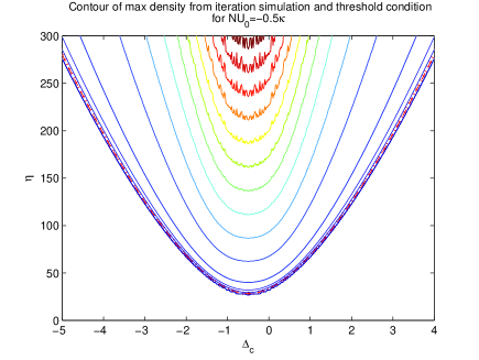
Fig. 1: Contour lines of the maximum of the selfconsistent atom density distribution for a cloud at rest as a function of detuning $\delta_{c}$ and pump amplitude $\eta$. The analytic formula for the the selforganization threshold is indicated by the red dashed line. Parameters are $N=200,U_{0}=-1/400,\kappa=1.$

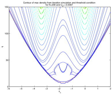
Fig. 2: Same as Fig. 1 for $N=200,U_{0}=-1/115,\kappa=1.$

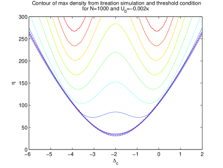
Fig. 3: Same as Fig. 1 for $N=1000,U_{0}=-1/375,\kappa=1.$

Let us now further substantiate these predictions for some special parameter choices by a real space dynamical solution of the equation of motion of N particles and the field modes. For this we use a semiclassical dynamical model as developed in ref. [3], where the atoms are modeled by polarizable point particles and the fields are amplitudes are represented by coherent states. This model has already been successfully applied to simulate cavity enhanced laser cooling and atomic selforganization in a standing wave cavity geometry[23]. Starting from a flat thermal distribution atomic distribution and with zero field amplitude, we then simply monitor the coupled atom-field evolution for a set of typical parameters. Due to the large number of variables we have to restrict ourselves to monitor only some characteristic observable like the evolution of the total kinetic energy, the magnitude of the bunching or the time evolution of the center of mass of the cloud. This is shown in Fig.4 where we compare contour lines the kinetic energy gain of the gas after a time of $\kappa t=60(check)$ with the analytic threshold formula from above. Indeed selfordering and significant acceleration of the particles is found only above the analytic threshold line.

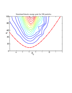
Fig. 4: Contour lines of kinetic energy gain of N=200 particles with average initial velocity zero and average kinetic energy $\hbar\kappa$ and $U_{0}=-0.015\kappa$ within a fixed time interval $\kappa t=60$.

4.2 Quasistationary accelerated particle distribution

As we now found a condition for the breakdown of stability of a homogeneous distribution, the next big question now is what happens in this instable regime? What kind of dynamics can we expect in general and under what conditions can we expect selforganization and an ordered accelerated particle distribution?

Obviously the backscattered field amplitude gets nonzero and the center of mass of the cloud gets accelerated. As a first guess for the further evolution we will now simply iterate the above loop further and see under which conditions a self consistent accelerated atom field distribution could possibly form. As we have no reliable time scales for the atomic thermalization process available, we will simply assume that it is faster than the time scale of significant acceleration of the cloud so that we keep the average velocity constant in these iterations.

Experimentally and in numerical simulations it has been found that in particular the regime $NU_{0}\geq\kappa$ has the biggest potential for a self ordered phase and interesting dynamics, so we will primarily focus on this regime[23].

In general for a wide range of parameters a self consistent accelerated atom field distribution can be found at a sufficient pump strength. A plot of the density distribution below, at, and above pump threshold is shown in Fig 5.

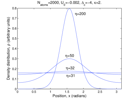
Fig. 5: Self consistent atomic density distribution below and above threshold for $N=2000$ atoms for $U_{0}=-0.001\kappa$ and $\delta_{c}=-2\kappa$. The analytic threshold result for this set of parameters is $\eta_{thresh}=31.6.$

Actually the iterations show, that the onset of self ordering depends non trivially on all the parameters and clear indications can already be seen even after only about five iterations. Typical numerical results can be visualized by plotting the peak atomic density versus pump strength for 5, 10 and 100 iterations as in Fig 6. There are no significant differences in convergence between 50 and 100 iterations. This peak density is a good indicator of atomic ordering, which due to translational invariance may form at any location between the mirrors. Alternatively the self consistent backscattered intensity turns out to be a good indicator for the onset of self ordering as a function of pump strength. From this quantity we can also determine the average force on the cloud.

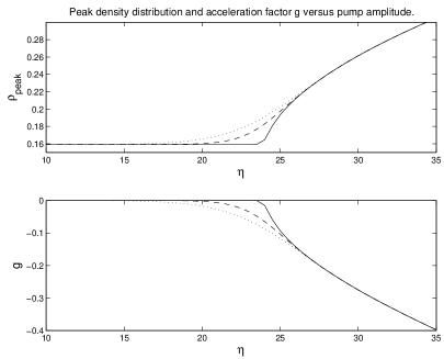
Fig. 6: Maximum atomic density as a function of pump amplitude for three different iteration numbers of 5 for dotted line, 10 for dashed line, and 100 for solid line.

The self ordering threshold can be located in Fig 6 or from the contour plots such as Fig 2 or 3 via the transition from the flat homogeneously distributed background to the exponential increase of local particle density. The transition is easy to see by eye. Numerically we have to select some value of particle density larger than the homogenous density and above the ”noise background” as an indicator of selforganization. In this way we can generate contour lines of the maximum density of the self consistent particle density. This allows a good comparison with the analytic form for the pumping threshold as a function of other parameters such as detuning. A plot of the density distribution below, at, and above threshold is shown in Fig 2. The key feature to note in Figs 2 and 3 is that in accordance with the analytical results derived above, the minimum threshold which occurs, when $\Delta_{c}=NU_{0}$, with a symmetric increase around this minimum. In seems that for a large range of parameters the instability of the flat distribution is connected with the existence of an ordered accelerated phase which is particularly stable for $\Delta_{c}<NU_{0}$.

A decrease of cavity damping leads to a sharper resonance of backscattered light at certain values of cavity detuning. We can estimate the value of cavity detuning which leads to the maximum backscattering (and average force) while holding other parameters fixed by taking the derivative of $\left|a_{-}\right|^{2}$,

$$\Delta_{c\text{ }Fmax}=NU_{0}\pm\sqrt{N^{2}U_{0}^{2}\left|R_{-}\right|^{2}-\kappa^{2}}$$ (26)

Recall the bunching parameter approaches unity here.  This result is only useful for small damping, $\kappa<NU_{0},$ where there is a distinct, sharp maxima of $\left|a_{-}\right|^{2}$ in the numerical results at $\Delta_{c}=0$ and $\Delta_{c}=2NU_{0}$ (with very little backscattering at $\Delta_{c}=NU_{0}).$  Thus as seen in Fig. 7 there are effectively these two resonant frequency of the cavity, with a larger Q leading to more backscattered light, but over a narrower $\Delta_{c}$ frequency interval.

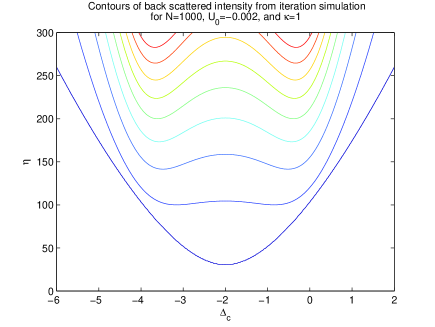
Fig. 7: Intensity of backscattered field mode as a function of detuning $\delta_{c}$ and pump amplitude $\eta$ for $N=1000$ atoms $U_{0}=-0.002\kappa$

Alternatively, for larger values of damping, $\kappa>NU_{0},$ the numerical results for backscattering show a maximum value at $\Delta_{c}=NU_{0}$ which decreases slowly away from this value of detuning. The limit on the overall range of cavity detuning which still permits self ordering of the particles is set by the pump.  The threshold pump value given in Eqs 25 and 24 should be exceeded to observe these backscattering dependencies on detuning.

To get some quantitative comparison with the selfconsistent atomic distributions calculated by the above iteration procedure and direct numerical simulations, we now also depict a contour plot the maximum of the atomic density distribution of a cloud of $N=1000$ atoms $NU_{0}=-2\kappa$ after a given time interval $\Delta t=xx/\kappa$ . We see that clear signs of selforganization appear when we cross the theoretically found threshold condition depicted as the line with crosses as a function of detuning and pump strength. We also see that crossing the threshold and ordering is accompanied by acceleration as expected.

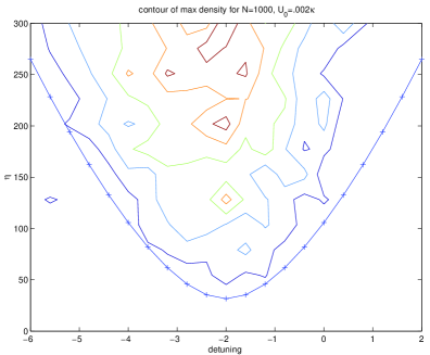
Fig. 8: maximum of atomic density distribution

4.3 Threshold conditions and deceleration prospects for a moving thermal cloud

Having investigated the dynamics of a gas at rest in some detail, we now come back to one of our original central goals and check the possibility of trapping and cooling molecules from a beam by superradiant scattering. In a typical setup one would send a molecular beam through the cavity in a small angle almost parallel to the ring cavity axis and inject a strong counter propagating coherent field. In such a setup the molecules are initially moving quite fast (up to ~100 m/s) with constant spatial density. The central question now is for which phase space densities, velocities and pump amplitudes superradiant scattering will appear and can be used slow down and trap the molecules.

In general using the rest frame of the beam the equations are the same as above except for different detunings $\Delta_{\pm}=\Delta_{c}\pm kv.$ for both cavity modes. Hence one can expect a similar threshold behavior. Naturally for a large value of the ratio of $kv/\kappa$ the pump and the backscattered field cannot be on resonance simultaneously. This will increase the threshold or even make self ordering not be possible. In principle on has the two possibilities of resonant pumping but a non resonant backscattered field or off resonant pumping to get resonant enhanced of the backscattered field.  The threshold for self ordering is first calculated assuming the cloud velocity is constant throughout the iteration.  We can compare this result to the threshold obtained using the accelerated frame where the velocity is updated throughout the iteration.

The most notable feature of the numerical results as seen in Fig. 9 is the asymmetry in the pumping threshold  with detuning as compared to the case with particles at rest.

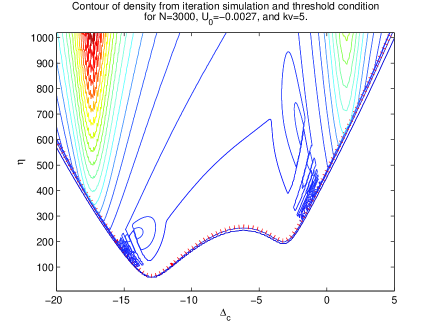
Fig. 9: Contour lines of maximum of the self consistent atomic density for $N=3000$ atoms for $U_{0}=-0.0017\kappa$ and $kv=5\kappa$. For comparison we also show the analytical expression for the selforganization threshold amplitude multiplied by 3 (dotted line).

Additionally, the analytic stability analysis leads to a first order stability equation for optical pumping threshold given by Eq. 23

For $NU_{0}>\kappa$ there is once again excellent agreement between the numerical and analytic results for pumping threshold as shown in Fig. 9 with only about a two percent difference in threshold values.  Trapping molecular beams with relatively large velocities is possible with a large pump and large cavity decay rate.  In this region where $NU_{0}<\kappa$, the analytic and numerical results for threshold are less in agreement, although the results have the same functional form as $kv$ increases.The backscattered intensity as a function of pumping versus velocity of the moving cloud is shown in Fig. 7.

4.4 Numerical multiparticle simulations of cold beam stopping

As a final check and demonstration of the efficiency of the setup we will now present some results on the possibility to stop a fast beam in such a setup again using real space simulations. In this case we start with beam of N=3000 particles in a thermal distribution of temperature $kT=\hbar\kappa$ but with additional average momentum of $p_{z}=-2000\hbar k$ per particle in the negative z-direction counter propagating the pump. As a measure of the efficiency of the scheme we first plot the amount of average kinetic energy extracted from the atoms by the fields in a time interval $\kappa t=60$ as a function of pump strength $\eta$ and pump detuning $\Delta_{c}$.

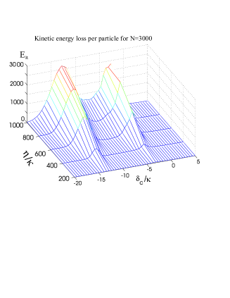
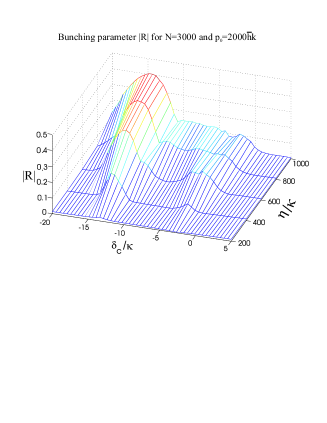
Fig. 10: (a) Kinetic energy loss per particle within a time interval of $\kappa t=60$ as a function of detuning $\Delta_{c}$ and pump amplitude $\eta$ for $N=3000$ atoms counterpropagating the cavity axis with initial average momentum of $p_{0}=2000\hbar\kappa$ and temperature $kT_{0}=\hbar\kappa$ and (b) average bunching parameter during this time for the same parameters.

Obviously we get efficient deceleration of the cloud when either the pump mode directly or the reflected light field is in resonance with the effective cavity eigenfrequencies[10]. When we plot the time averaged bunching parameter we see that efficient energy transfer is associated with atomic selfordering as analytically predicted. As the atomic bunching is more efficient for negative detunings we get a more efficient energy extraction in this limit.

These results compare qualitatively quite well with the analytic prediction of Eq.23 as shown in Fig.11 where we compare a contour plot of bunching parameter with the analytic threshold formula for the selforganization threshold multiplied by 3 (line with crosses).

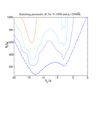
Fig. 11: Contour lines of time averaged bunching parameter $|R|$ found by numerical simulation as function of detuning $\delta_{c}$ and pump amplitude $eta$ for parameters above. Again for reference we show the analytical result for the selforganization threshold (x3)

5 Conclusions

We studied the conditions to stop and trap a fast molecular beam by help of a single side pumped high Q ring cavity geometry in a CARL setup. The analytical results for kinetic energy extraction from a self consistent stationary solution of the coupled particle field equations were checked by numerical simulations. In the limit of large detuning inversion is negligible and coherent light scattering dominates. As the atom field interaction strength per particle is small in this regime we need collective enhancement of the Raleigh scattering blue shifted with respect to the excitation light to do the job. This can be achieved in a regime where the particles arrange in a periodic density lattice and form a moving Bragg mirror.

Finding the effective optical potential in an accelerated frame and applying a linear stability analysis allows to derive the analytic threshold for the laser pump power, above which an initial homogenous particle distribution gets unstable against small density fluctuations. We see that the available phase space density at the beginning determines the required threshold laser intensity. Above this threshold a suitable choice of detunings causes the interference of the injected and collectively backscattered light fields to establish a periodic particle density acting like a moving Bragg mirror, which yields a time dependent coupling of the counter propagating fields within the resonator. By using a mean-field analysis the self consistent atom-field distribution is found by an iteratively which allows to quantitatively predict the maximal acceleration and localization of the cloud.

In a second step we checked these predictions by simulating the microscopic equations of motions of the particles for finite ensembles. These simulations show surprisingly good qualitative and quantitative agreement with the analytic threshold result and acceleration predictions within the regime, where the analytical model predicts selforganization. Outside this regime, where the effective potential in the accelerated frame shows no periodic local minima the simulations differ from the analytic predictions. This can be traced to cavity induced heating processes in this regime as well as remnant radiation pressure not accounted for in the analytic model. In any case the analytically found threshold formula for the selforganization process provides a solid criterion for the prospects of a corresponding experimental setup.

As a bottom line trapping and stopping of a fast molecular beam in a ring cavity seems experimentally feasible with current technology, provided one can find a strong enough pump laser at a frequency where the particles are polarizable but sufficiently transparent. The higher the initial phase space density of the particles, the faster this process will happen and the stronger are the deceleration forces and the suppression of spontaneous emission. In favorable cases this could be combined with cavity cooling in the particles rest frame as well[3].

This work could be extended by continuing the work of Asbóth who has used the mean field analysis to find self-organization thresholds in standing wave cavities, but now analyzed with transverse mode degeneracy.  In particular, Vuletić’s group has found the degeneracy of a confocal resonator significantly enhances the cooling efficiency.  It would be useful to examine such threshold behavior in this highly degenerate regime.