Quantum simulation of spin ordering with nuclear spins in a solid state lattice

Abstract

An experiment demonstrating the quantum simulation of a spin-lattice Hamiltonian is proposed. Dipolar interactions between nuclear spins in a solid state lattice can be modulated by rapid radio-frequency pulses. In this way, the effective Hamiltonian of the system can be brought to the form of an antiferromagnetic Heisenberg model with long range interactions. Using a semiconducting material with strong optical properties such as InP, cooling of nuclear spins could be achieved by means of optical pumping. An additional cooling stage is provided by adiabatic demagnetization in the rotating frame (ADRF) down to a nuclear spin temperature at which we expect a phase transition from a paramagnetic to antiferromagnetic phase. This phase transition could be observed by probing the magnetic susceptibility of the spin-lattice. Our calculations suggest that employing current optical pumping technology, observation of this phase transition is within experimental reach.

I Introduction

Many-body problems are common in condensed matter physics. However, computations of interesting quantities, such as critical exponents of a phase transition, are difficult, specifically because the dimension of the associated Hilbert space increases exponentially with the system size. Recent quantum simulation experiments using cold atoms in an optical lattice Greiner et al. (2002); García-Ripoll et al. (2004) have opened new possibilities for the study of these systems. The idea consists of controlling the interactions inside a many-body system so that they take a desired form, and performing measurements on the macroscopic behavior of the system. It is interesting to explore how this quantum simulation concept could be implemented in different physical systems.

Spin-lattice models are a convenient, simple model to describe magnetic phenomena Stanley (1987). It was recently realized, however, that various apparently unrelated problems can be cast into this same language. An example is the half-filled Hubbard model in the limit of large positive on-site Coulomb repulsion $U$ Auerbach (1998). This observation makes spin-lattice models interesting not only for fundamental studies of magnetism, but also as a means to attack several other problems. Although spin-lattice models have been studied for about a century, exact results only exist for special cases of low spatial dimensionality. Approximation methods such as mean-field theory offer an alternative, but they typically involve assumptions that are not rigorously justified. On the other hand, numerical methods such as Monte Carlo simulation Landau and Binder (2005) have limited efficiency for calculations in real three-dimensional magnetic systems. This motivates the investigation of other techniques to study spin-lattice models.

In this paper, we consider a solid-state lattice of nuclear spins as a simulator of a specific spin-lattice model, in which interactions between spins are modulated by rapid radio-frequency pulses. The potential of nuclear magnetic resonance (NMR) techniques Ramanathan et al. (2004); Abragam (2004) for simulating an artificial many-body Hamiltonian is theoretically explored. Nuclear spins interact predominantly via a magnetic dipolar interaction, which can be modulated by varying the orientation of the crystal relative to the applied magnetic field, applying NMR pulse sequences, or using different material systems. By optically cooling the nuclear spins Meier and Zakharchenya (1984); Tycko and Reimer (1996), or by implementing a similar dynamic polarization technique, it is possible that the system eventually reaches a nuclear spin temperature Abragam (2004); Abragam and Proctor (1958); Goldman (1970) where a phase transition Stanley (1987) occurs. In particular, in Sec. V we describe the transition from a paramagnetic to an antiferromagnetic phase that we expect to occur in our proposed system. In this context, we are not considering a generic spin-Hamiltonian simulator, but rather a problem-specific machine, where we have the ability to change some aspects of the spin-lattice Hamiltonian and the spin temperature, using the freedom provided by the particular experimental system.

The proposed experiment proceeds as follows: We first optically pump a sample of bulk InP in low physical temperature and high magnetic field, so that the resulting nuclear-spin polarization is maximum Michal and Tycko (1999); Goto et al. (2004). We then perform adiabatic demagnetization in the rotating frame (ADRF) to transfer the Zeeman order to the dipolar reservoir Slichter (1990); Oja and Lounasmaa (1997). This is a cooling technique analogous to slowly switching off the dc magnetic field in the laboratory frame. If it is performed adiabatically, i.e. with no loss of entropy, the ordering due to alignment of the spins along the dc magnetic field is transferred to ordering due to local correlations of the spin orientations. By applying a suitably chosen NMR pulse sequence, we can transform the inherent Hamiltonian of the system to the desired one in an average sense, to be described below. In particular, we use NMR techniques to engineer an antiferromagnetic Heisenberg model with long range interactions. This transformation is validated by average Hamiltonian theory (AHT) Haeberlen (1976). Our system has two species of nuclear magnetic moments. We argue that in the ground state of the described Hamiltonian each nuclear species is ordered antiferromagnetically, so that each nuclear species consists of two sublattices of opposite spin orientation. Antiferromagnetic ordering with two sublattices can be observed in the NMR spectrum as the appearance of two peaks of opposite phase: In a system with two nuclear species A and B of widely-separated Larmor frequencies, we can rotate the spins A to the horizontal plane using a $\frac{\pi}{2}$-pulse, and observe their free induction decay (FID) signal. If the spins B are in an antiferromagnetically ordered state, they create a spatially oscillating local field that modulates the Larmor frequency of spins A. This means that spins A in different sublattices will produce the FID signals of different frequencies. However, to decide whether a phase transition occurs, we need to measure the magnetic susceptibility of the system Goldman et al. (1974); Mouritsen and Jensen (1980). In particular, the longitudinal susceptibility has a maximum at the transition temperature, while the transverse susceptibility exhibits a plateau inside the ordered phase. Nuclear spin susceptibilities can be easily extracted from the Fourier-transformed FID signals recorded after a short pulse. This measurement exploits the Fourier-transform relationship between transient and steady-state response of a system to a small perturbation.

All individual pieces of this experiment have already been demonstrated, but putting them together is challenging. Nuclear ordering has been observed in a series of experiments Oja and Lounasmaa (1997); Chapellier et al. (1970); Quiroga et al. (1983a, b). However, the effect of NMR pulse sequences to engineer an artificial Hamiltonian has not been studied in detail, and this is an issue that the current study addresses. We should note that the class of Hamiltonians that can be simulated with this method is severely limited by the characteristics of the particular material system, although many interesting cases can be studied, for example frustrated spin lattices.

This paper is organized as follows: In Sec. II, we briefly describe adiabatic demagnetization in the rotating frame (ADRF), which is essentially a cooling technique for nuclear spins. Sec. III discusses the calculation of thermodynamic quantities for systems obeying the spin Hamiltonians of interest, and in particular, the evolution of spin temperature during ADRF in our proposed material system. In this way, we can calculate the spin temperature reached by the spin-lattice after ADRF. In the subsequent two sections, we describe the spin Hamiltonians that can be simulated by this method. In particular, a suitable NMR pulse sequence is discussed in Sec. IV, and an experimental material system is presented in Sec. V. Finally, in Sec. VI, we give an estimate, based on mean-field approximation, of the initial polarization needed to observe a phase transition.

II Description of adiabatic demagnetization in the rotating frame (ADRF)

The term adiabatic is used in two different meanings in physics, one quantum mechanical, and the other thermodynamic Abragam (2004); Abragam and Proctor (1958). ADRF is based on the thermodynamic definition, which is a reversible process with no heat transfer, in which the entropy of the system remains constant. The term isentropic also applies to this case. By contrast, in quantum mechanics, the term adiabatic usually means that the relative populations of the various energy eigenstates of the system are kept constant. The two definitions are in general incompatible.

The system of nuclear spins interacts only weakly with the crystal lattice. The relevant timescale for this interaction is $T_{1}$ Abragam (2004). So, if we are interested in phenomena much faster than $T_{1}$, we can treat the system as being effectively isolated, and describe it in terms of its nuclear spin temperature Goldman (1970), which can be very different from the lattice temperature. Of course, if we let the system to relax over several timescales $T_{1}$, these two temperatures eventually become equal.

Consider a lattice of nuclear spins in a dc Zeeman magnetic field $B_{0}$ along the $z$-direction. During ADRF, we apply a rotating radio-frequency (rf) magnetic field in the $x$-$y$ plane of magnitude $B_{1}$ and angular frequency $\omega_{1}$, so that the Hamiltonian in the frame rotating with angular frequency $\omega_{1}$ (rotating frame) is

$$\mathcal{\hat{H}}^{rot}=-\sum_{i}\hbar\left[\left(\gamma_{i}B_{0}-\omega_{1}\right)\hat{I}_{i}^{z}+\gamma_{i}B_{1}\hat{I}_{i}^{x}\right]+\mathcal{\hat{H}}^{\prime}_{D},$$ (1)

where $\hat{I}^{x,y,z}_{i}$ and $\gamma_{i}$ are the spin operators and gyromagnetic ratio of the $i^{\text{th}}$ spin dipole, and $\mathcal{\hat{H}}^{\prime}_{D}$ denotes the secular part of the dipolar interaction Hamiltonian. The latter follows after dropping the rapidly oscillating terms. The three terms in the above equation we called the Zeeman, the rf (radio frequency), and the dipolar part of the total Hamiltonian, respectively. In the case where the lattice consists of nuclear spins of the same species Slichter (1990)

$$\mathcal{\hat{H}}^{\prime}_{D} =\frac{\mu_{0}}{4\pi}\hbar^{2}\gamma_{I}^{2}\frac{1}{2}\sum_{i\neq j}\frac{1-3\cos^{2}(\theta_{ij})}{r_{ij}^{3}}\left(\hat{I}_{i}^{z}\hat{I}_{j}^{z}-\frac{1}{2}\hat{I}_{i}^{+}\hat{I}_{j}^{-}\right)$$

$$\equiv\frac{1}{2}\sum_{i,j}u_{ij}\left(\hat{I}_{i}^{z}\hat{I}_{j}^{z}-\frac{1}{2}\hat{I}_{i}^{+}\hat{I}_{j}^{-}\right)=\mathcal{\hat{H}}^{\prime}_{II}.$$ (2)

The distance between the spins $i$ and $j$ is $r_{ij}$, $\theta_{ij}$ is the angle between the vector $\bm{r}_{ij}$ and the direction of the Zeeman magnetic field $\hat{z}$, while $\hat{I}_{i}^{\pm}=\hat{I}_{i}^{x}\pm i\hat{I}_{i}^{y}$ and $\gamma_{I}$ is the common gyromagnetic ratio of the spins . Note the role of the term $-\sum_{i}\hbar\gamma_{i}B_{1}\hat{I}_{i}^{x}$ in (1) allowing the Zeeman and dipolar reservoirs to exchange energy. In the absence of the rf field, the Zeeman and dipolar parts of the Hamiltonian are separate constants of motion, and the conditions of thermal equilibrium are not satisfied. In the presence of the rf field, a common spin-temperature is established, and the system is described in the rotating frame by the density matrix

$$\hat{\rho}^{rot}=\frac{\exp\left(-\beta\mathcal{\hat{H}}^{rot}\right)}{\mathrm{Tr}\left[\exp\left(-\beta\mathcal{\hat{H}}^{rot}\right)\right]}.$$ (3)

The process of establishment of thermal equilibrium is described by the Provotorov equations Abragam and Goldman (1982). When the rf term becomes comparable to the Zeeman term, Zeeman order is established along the direction of the effective magnetic field $\left(B_{0}-\frac{\omega_{1}}{\gamma_{I}}\right)\hat{z}+B_{1}\hat{x}$. After $\omega_{1}$ reaches $\gamma_{I}B_{0}$, we switch off the rf field $B_{1}$ adiabatically, so that all the initial Zeeman order is transferred to the dipolar reservoir.

III Evolution of spin-temperature during ADRF

During ADRF, the entropy of the system remains constant. So, if we have an expression for the entropy as a function of the inverse spin-temperature $\beta$, we can calculate the spin-temperature during the ADRF. In particular, we can estimate the desired initial polarization, that is required in order to observe a phase transition.

In the rest of the paper, we drop the superscript ${rot}$, as we are only going to work in the rotating frame. We also use the word temperature to denote nuclear spin-temperature.

In the high temperature approximation Slichter (1990), we can expand the expression for the density matrix (3) to first order in inverse temperature $\beta$

$$\hat{\rho}=A\left(\hat{1}-\beta\mathcal{\hat{H}}\right).$$ (4)

where $A$ is a suitably chosen constant, so that $\rm{Tr}(\hat{\rho})=1$. The entropy $\mathcal{S}$ then follows from the equation

$$\mathcal{S}=-k_{B}\mathrm{Tr}\left(\hat{\rho}\ln\hat{\rho}\right).$$ (5)

For $N$ spin-$j$ particles of the same species, with gyromagnetic ratio $\gamma$, interacting through the dipolar interaction of eq. (2) we find, in the rotating frame

$$\frac{\mathcal{S}}{Nk_{B}}=\ln(2j+1)-\beta^{2}\hbar^{2}\gamma^{2}\frac{j(j+1)}{6}\left[\left(B_{0}-\frac{\omega_{1}}{\gamma}\right)^{2}+B_{L}^{2}\right],$$ (6)

where

$$B_{L}^{2}\equiv\frac{3}{4}\frac{j(j+1)}{3\hbar^{2}\gamma^{2}}\sum_{j}\left(u_{ij}\right)^{2}.$$ (7)

In the above equation, we have ignored the rf field $B_{1}$. $B_{L}$ can be interpreted as a “local field” due to the neighboring spins.

We follow the procedure described in Refs. Goldman et al., 1975; Stinchcombe et al., 1963; Abragam and Goldman, 1982 (see also Ref. Izyumov and Skryabin, 1988 for similar calculations) to extend this description to the case of lower temperature. The idea is to include more terms in the expansion (4), applying a diagrammatic technique similar to that used in perturbation theory. The Zeeman term is considered as the free part of the Hamiltonian, and is treated to all orders. The dipolar interaction term is considered as the perturbation, and by grouping the resulting terms using a procedure that recalls Wick’s theorem Wick (1950), we are able to efficiently perform the summations. In this calculation, we ignore the rf term in (1), as this has only the effect of bringing the Zeeman and dipolar reservoirs to equilibrium. Also, far from resonance, the two spin species cannot exchange energy, because their interaction takes the form $\sum_{ik}v_{ik}\hat{I}_{i}^{z}\hat{S}_{k}^{z}$, which cannot induce flip-flops. When the rf part in equation (1) becomes comparable with the Zeeman part, the two reservoirs can exchange energy, because in this case the Zeeman ordering is not along the $\hat{z}$ direction. This means that the Zeeman and interaction parts of the Hamiltonian do not commute, so they are not separately constants of motion, and the conditions for the establishment of thermal equilibrium are satisfied. In our approximation, we do not study the effect of different spin-temperatures. Our calculation consists of defining the initial polarization of one spin species, and calculating the spin-temperature in the rotating frame during the ADRF, with the constraints that the system is described by one spin-temperature, and that the entropy is invariant.

To study the feasibility of observing a phase transition, we estimate $T_{c}$ by the condition that the longitudinal magnetic susceptibility vanishes, as the ordered state is expected to be an antiferromagnet. This is not an accurate calculation, however, because only a few diagrams are involved in the high-temperature expansion, while in the critical region higher order terms become increasingly important. A common procedure to take the latter into account is described in Ref. Stanley, 1987, in which extrapolation procedures are used to compute the limiting behavior of high-temperature expansion series given only the knowledge of the first few terms. Also, antiferromagnets have a more rich phenomenology than this simple picture. In particular, Refs. Haldane, 1983a, b; Auerbach, 1998 imply that 1D Heisenberg antiferromagnetic spin chains, in the limit of large spin, are gapless for half-integer spin, so that the susceptibility does not vanish at the critical point. The mean-field description Goldman et al. (1974) is quite different, as well. A much better way, based on mean-field theory, to calculate critical quantities, is presented in Sec. VI.

III.1 The longitudinal case

Assume that the spin interaction is longitudinal; that is, the Hamiltonian has the form

$$\mathcal{\hat{H}}=\Delta\sum_{i}\hat{I}_{i}^{z}+\frac{1}{2}\sum_{i,j}u_{ij}\hat{I}_{i}^{z}\hat{I}_{j}^{z}\equiv\mathcal{\hat{H}}_{Z}+\mathcal{\hat{H}}^{\prime}.$$ (8)

$\Delta$ stands for the detuning $\hbar\left(\gamma_{I}B_{0}-\omega_{1}\right)$. After thermalization, the system is described by the density matrix

$$\hat{\rho}=\frac{\exp\left(-\beta_{0}\mathcal{\hat{H}}_{Z}-\beta\mathcal{\hat{H}}^{\prime}\right)}{\mathrm{Tr}\left[\exp\left(-\beta_{0}\mathcal{\hat{H}}_{Z}-\beta\mathcal{\hat{H}}^{\prime}\right)\right]}.$$ (9)

We allow for different temperatures for the Zeeman and dipolar reservoir for convenience in the calculation. In the end, we are going to set these temperatures equal. Defining the zeroth order thermal average for an operator $\mathcal{\hat{Q}}$ as

$$\langle\mathcal{\hat{Q}}\rangle_{0}=\frac{\mathrm{Tr}\left[\exp\left(-\beta_{0}\mathcal{\hat{H}}_{Z}\right)\mathcal{\hat{Q}}\right]}{\mathrm{Tr}\left[\exp\left(-\beta_{0}\mathcal{\hat{H}}_{Z}\right)\right]},$$ (10)

and treating the interaction term as a perturbation, we have the following expansion for the true thermal average

$$\langle\mathcal{\hat{Q}}\rangle=\frac{\sum_{n=0}^{\infty}\left(-\beta\right)^{n}\langle\left(\mathcal{\hat{H}}^{\prime}\right)^{n}\mathcal{\hat{Q}}\rangle_{0}/n!}{\sum_{n=0}^{\infty}\left(-\beta\right)^{n}\langle\left(\mathcal{\hat{H}}^{\prime}\right)^{n}\rangle_{0}/n!}.$$ (11)

$\left(\mathcal{\hat{H}}^{\prime}\right)^{n}$ involves multiple sums, and the bookkeeping becomes complicated, unless we define the semi-invariants $M^{0}_{i}$

$$\langle(\hat{I}_{j}^{z})^{n}\rangle_{0}=\sum_{i_{1}+i_{2}+\ldots+i_{p}=n}M^{0}_{i_{1}}M^{0}_{i_{2}}\ldots M^{0}_{i_{n}}.$$ (12)

With this definition, we can write down a diagrammatic expansion, like the one described in Ref. Stinchcombe et al., 1963. The advantage over the brute-force expansion (11) is that the resulting sums are unrestricted, i.e. no constraints such as $i\neq j$ are involved in the summations. If we define connected diagrams as those involving $\mathcal{\hat{Q}}$, and disconnected ones as those not involving it, we can factor the numerator as the product of the sum of connected diagrams times the sum of disconnected ones. The latter serves to cancel the denominator, so that only connected diagrams matter.

The calculation of the semi-invariants is straightforward. With the definitions

$$\eta =-\beta_{0}\Delta,$$

$$f_{j}(\eta) =\mathrm{tr}\left(e^{\eta\hat{I}^{z}}\right)=\frac{\sinh\left[\eta\left(j+\frac{1}{2}\right)\right]}{\sinh\left(\frac{\eta}{2}\right)},$$ (13)

$$t_{j}^{(n)} =\frac{1}{f_{j}(\eta)}\left(\frac{\mathrm{d}}{\mathrm{d}\eta}\right)^{n}f_{j}(\eta),$$

the first few semi-invariants can be written as

$$M^{0}_{1} =t_{j}^{(1)},$$ (14a)

$$M^{0}_{2} =t_{j}^{(2)}-\left(t_{j}^{(1)}\right)^{2},$$ (14b)

$$M^{0}_{3} =t_{j}^{(3)}-3t_{j}^{(2)}t_{j}^{(1)}+2\left(t_{j}^{(1)}\right)^{3}.$$ (14c)

The general case is covered in Appendix A

III.2 Calculation of thermodynamic quantities

In this subsection, we calculate the entropy as a function of inverse temperatures $\beta$ and $\beta_{0}$ and detuning $\Delta$. In the final formulas, we always set $\beta_{0}=\beta$, but we consider $\beta$ and $\beta_{0}$ as independent variables in the calculation of derivatives. We first need to calculate the average polarization.

$$\Delta\frac{\partial}{\partial\beta}\langle\hat{I}^{z}\rangle=\frac{\partial}{\partial\beta_{0}}\langle\mathcal{\hat{H}}^{\prime}_{D}\rangle=\frac{\partial}{\partial\eta}\langle\mathcal{\hat{H}}^{\prime}_{D}\rangle\frac{d\eta}{d\beta_{0}}=-\Delta\frac{\partial}{\partial\eta}\langle\mathcal{\hat{H}}^{\prime}_{D}\rangle.$$ (15)

The dipolar interaction energy $\langle\mathcal{\hat{H}}^{\prime}_{D}\rangle$ is calculated in Appendix B in terms of the functions $G_{n}(.)$ defined there. Performing the integral in the above equation, we find

$$\frac{\langle\hat{I}^{z}\rangle(\beta_{0},\beta)}{N}=t^{(1)}\\ -\sum_{n}\frac{\beta^{n+1}}{n+1}\frac{\partial}{\partial\eta}G_{n}\left(t^{(1)}(\eta),t^{(2)}(\eta),\ldots,t^{(n+1)}(\eta)\right).$$ (16)

If we keep terms to first order in $\Delta$, we can estimate the longitudinal magnetic susceptibility.

$$\frac{1}{N}\langle\hat{I}^{z}\rangle\simeq\\ -(\beta\Delta)\frac{j(j+1)}{540}\left[180-(33+56j+56j^{2})\beta^{2}\left(\gamma\hbar B_{L}\right)^{2}\right].$$ (17)

This formula provides a method to estimate the critical temperature of the paramagnetic to antiferromagnetic phase transition from the temperature at which the susceptibility becomes zero. For spin-$\frac{1}{2}$ and spin-$\frac{9}{2}$, we find

$$k_{B}T_{C}(j=\frac{1}{2})=0.645\left(\gamma\hbar B_{L}\right),$$ (18a)

$$k_{B}T_{C}(j=\frac{9}{2})=2.81\left(\gamma\hbar B_{L}\right).$$ (18b)

This is a very rough estimate, as discussed in the beginning of this section. Further, it refers to the ordering of each species in its own lattice, not involving coupling between them. Eventually we will use these couplings to create the artificial Hamiltonian described in Sec. IV.

The free energy follows from the expression

$$\ln\mathcal{Z}(\beta_{0},\beta)=\ln\mathcal{Z}(\beta_{0},0)-\int_{0}^{\beta}\langle\mathcal{\hat{H}}^{\prime}_{D}\rangle(\beta_{0},\lambda)d\lambda,$$ (19)

which can be expressed in terms of the functions $G_{n}$

$$\frac{1}{N}\ln\mathcal{Z}(\beta_{0},\beta)=\ln f_{j}(-\beta_{0}\omega_{0})\\ -\sum_{n}\frac{\beta^{n+1}}{n+1}G_{n}\left(t^{(1)}(\eta),t^{(2)}(\eta),\ldots,t^{(n+1)}(\eta)\right).$$ (20)

We are now ready to calculate the entropy.

$$\frac{\mathcal{S}}{k_{B}}=\beta_{0}\omega_{0}\langle\hat{I}^{z}\rangle+\beta\langle\mathcal{\hat{H}}^{\prime}_{D}\rangle+\ln\mathcal{Z}(\beta_{0},\beta);$$ (21)

in terms of the functions $G_{n}$,

$$\frac{\mathcal{S}}{Nk_{B}}=-\eta t_{j}^{(1)}+\ln f_{j}(\eta)+\sum_{n}\frac{\beta^{n+1}}{n+1}\left(nG_{n}+\eta\frac{\partial}{\partial\eta}G_{n}\right).$$ (22)

III.3 Results

During ADRF, the entropy remains constant. In order to obtain an ordered final state, we need the initial state to be sufficiently polarized. A rough estimate for spin-$\frac{1}{2}$ species is to set the spin temperature $k_{B}T$ of the initial paramagnetic state equal to the level spacing $\hbar\gamma B_{0}$. This means that we need the initial polarization, which is defined as the thermal average magnetization over maximum magnetization, to be

$$p=\tanh\left(\frac{\hbar\gamma B_{0}}{2k_{B}T}\right)=0.46.$$ (23)

Sec. VI gives a better picture of how the initial polarization influences the ordering observed under the artificial Hamiltonian we wish to implement.

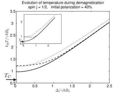
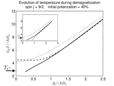
Figure 1: Evolution of spin temperature $T$ vs detuning $\Delta$ during ADRF. Dotted line: high temperature approximation. Broken line: first order approximation. Continuous line: second order approximation. These approximations are discussed in Sec. III and in the Appendices. Insets: Initial polarization of 50%. The parameter $B_{L}$ (local field) is defined in (7), $T_{c}$ is calculated in (18b). The calculation involves one spin species with spin-$\frac{1}{2}$ or $\frac{9}{2}$ in an fcc lattice and the Zeeman magnetic field along the (111) crystalline direction. For high initial polarization, large spin, and near resonance, the calculation does not converge.

In Fig. 1 we present the results of our numerical calculation. About 50% initial polarization of the spins is required in order to reach a spin temperature where a phase transition can be observed. Details about the proposed material system are presented in Sec. V and in the Appendices.

IV Pulse sequence and the artificial Hamiltonian

If the system has been sufficiently cooled via optical pumping and ADRF, it might be in dipolar-ordered state because of the inherent interaction between spins. On the other hand, by applying a WAHUHAWaugh et al. (1968); Haeberlen and Waugh (1968), or MREV8Mansfield (1971); Rhim et al. (1973a, b) pulse sequenceHaeberlen (1976) on resonance, we can decouple spins of the same species, and transform the interaction between unlike spins from an Ising-like interaction to a Heisenberg-like interaction.

In particular, the WAHUHA pulse cycle is given by

$$\tau-P_{x}-\tau-P_{-{y}}-2\tau-P_{y}-\tau-P_{-{x}}-\tau,$$ (24)

where $P_{\alpha}$ and $P_{-\alpha}$ denote $\frac{\pi}{2}$ and $-\frac{\pi}{2}$ pulses respectively around the $\alpha$-axis, ($\alpha=x,y$). $\tau$ and $2\tau$ denote the time interval between the application of consecutive pulses. The pulse cycle time is $t_{c}=6\tau$ plus the duration of the four pulses. MREV8 contains two WAHUHA-type pulse cycles, concatenated to mitigate pulse imperfection effects. If the pulses are short enough, then their effect can be modeled as an instantaneous transformation of the Hamiltonian. To first order in $t_{c}$ relative to the magnitude of the Hamiltonian, the system dynamics are described by the time-averaged Hamiltonian over the pulse cycle. Average Hamiltonian theory (AHT) is covered in detail in several textbooks (see, for example, Ref. Haeberlen, 1976). To first order in AHT, the dipolar interaction in the rotating frame between nuclei of the same species (2) is eliminated. If we simultaneously apply this pulse sequence to both species, their dipolar interaction in the rotating frame

$$\mathcal{\hat{H}}^{\prime}_{IS}=\sum_{i,k}w_{ik}\hat{I}_{i}^{z}\hat{S}_{k}^{z}$$ (25)

is transformed to a Heisenberg-like interaction

$$\hat{\overline{\mathcal{H}^{\prime}}}_{IS}=\sum_{i,k}w_{ik}\frac{1}{3}\hat{\bm{I}}_{i}\cdot\hat{\bm{S}}_{k}.$$ (26)

In the above sums, the index $i$ runs over the spins $I$, whereas the index $k$ runs over the spins $S$. $w_{ik}$ has a similar expression as $u_{ij}$ in (2).

$$w_{ik}=\frac{\mu_{0}}{4\pi}\hbar^{2}\gamma_{I}\gamma_{S}\frac{1-3\cos^{2}(\theta_{ik})}{r_{ik}^{3}}.$$ (27)

If we use the modified WAHUHA pulse cycle

$$\tau_{1}-P_{x}-\tau_{2}-P_{-{y}}-2\tau_{2}-P_{y}-\tau_{2}-P_{-{x}}-\tau_{1},$$ (28)

the effective interaction Hamiltonians to first order in AHT are

$$\hat{\overline{\mathcal{H}^{\prime}}}_{II}(\tau_{1},\tau_{2})=\frac{\tau_{1}-\tau_{2}}{t_{c}}\sum_{i,j}u_{ij}\left(\hat{I}_{i}^{z}\hat{I}_{j}^{z}-\frac{1}{2}\hat{I}_{i}^{+}\hat{I}_{j}^{-}\right)$$ (29)

$$\hat{\overline{\mathcal{H}^{\prime}}}_{IS}(\tau_{1},\tau_{2})=\sum_{i,k}w_{ik}\left[\frac{2\tau_{1}}{t_{c}}\hat{I}_{i}^{z}\hat{S}_{k}^{z}+\frac{2\tau_{2}}{t_{c}}\left(\hat{I}_{i}^{x}\hat{S}_{k}^{x}+\hat{I}_{i}^{y}\hat{S}_{k}^{y}\right)\right]$$ (30)

where $t_{c}=2\tau_{1}+4\tau_{2}$. By keeping $t_{c}$ constant and varying $\tau_{2}$ adiabatically from $0$ to $\frac{t_{c}}{6}$, we can get an interpolation between the initial and final Hamiltonians $\mathcal{\hat{H}}^{init}$, $\mathcal{\hat{H}}^{fin}$, and transform the state of the system from the thermal state of $\mathcal{\hat{H}}^{init}$ with entropy $\mathcal{S}$ to the thermal state of $\mathcal{\hat{H}}^{fin}$ with the same entropy. In this way, we can study the thermodynamics of the particular Heisenberg model for varying entropy. An alternative method is to keep $\tau_{1}=\tau_{2}$ and vary the width of the pulses, so that they induce rotations by an angle $\theta$, same for all pulses. By varying $\theta$ from 0 to $\frac{\pi}{2}$, we have a similar effect, but the equations for the effective interactions are more complicated.

V Choice of the experimental system

Bulk InP is a suitable material for this experiment. As described in Sec. IV, two spin species are required to implement the desired model Hamiltonian. A strained lattice, on the other hand, like a quantum well exhibits strong quadrupolar broadening. This is because spins higher than $\frac{1}{2}$, such as ¹¹³In and ¹¹⁵In, include a quadrupole term in the Hamiltonian, which gives a non-zero contribution in the presence of electric field gradients. When this contribution is the dominant one, it can be expected that any ordering due to the dipolar interaction term is destroyed. Phosphorous has only one isotope ³¹P with spin-$\frac{1}{2}$, while Indium has two isotopes, ¹¹³In and ¹¹⁵In have the same spin ($\frac{9}{2}$) and are close in Larmor frequency for typical NMR magnetic fields, so we can consider Indium to be homonuclear. InP is a direct-gap semiconductor with strong optical properties, and efficient optical cooling has already been demonstratedMichal and Tycko (1999); Goto et al. (2004). InP has a zincblende structure; if a dc magnetic field is applied along the (111) crystalline direction, and couplings between spins of the same species are neglected during the application of the NMR pulse sequence as described in Sec. IV, then the magnetic dipolar interaction between nuclei creates the following structure (note that the gyromagnetic ratio $\gamma$ of both In and P nuclei is positive). The planes of Indium and Phosphorous nuclei are grouped into pairs. The coupling between nearest neighbors (nn), which are always of different species, is antiferromagnetic if both nuclei belong to the same pair of planes, and ferromagnetic if the nuclei belong to successive pairs of planes. Second-nearest-neighbors are of the same spin species, and so their interaction is averaged out. Some third-nearest-neighbors interactions cause frustration, but the magnetic field orientation ensures that their effect is small. Ignoring interactions farther than third-nearest-neighbors, this leads the rather nice picture shown in Fig. 2. Interactions within each pair of planes are antiferromagnetic. Coupling between plane pairs is ferromagnetic. It is possible (but by no means certain) that in the absence of an offset dc magnetic field in the rotating frame, each plane pair acts as a two-dimensional antiferromagnet, where the ferromagnetic interaction between plane pairs merely ensures that all of them have the same structure. A complementary picture results if we consider each spin species independently. In our proposed structure, each species forms a lattice with antiferromagnetically ordered spins. Antiferromagnetic ordering within spins of the same species results in an indirect way through interactions with spins of the other species, as shown in Fig. 2.

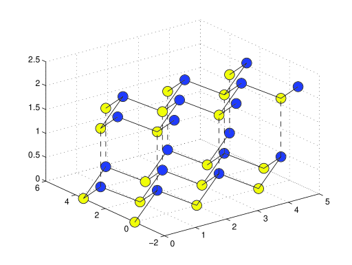
Figure 2: (color online) The configuration of the nuclear spins under the experimental conditions described in Sec. V. Spheres of the same color represent nuclei of the same species. Solid lines are antiferromagnetic bonds, while broken lines are ferromagnetic ones. Only nearest-neighbor bonds are plotted. The perpendicular direction in this figure is the (111) crystalline direction. We can see the postulated antiferromagnetic planes, which are coupled ferromagnetically. Within each plane, spins of one species tend to form a ferromagnetic lattice which is aligned antiferromagnetically to the lattice formed by the spins of the other species. On the other hand, spins of the same species belonging to successive planes tend to align antiferromagnetically.

How reasonable is it for us to neglect interactions beyond 3rd nn? The strength of dipolar interactions falls off with distance only as $\frac{1}{r^{3}}$, and because the volume integral

$$\iiint\mathrm{d}V\frac{1}{r^{3}}=4\pi\int_{0}^{\infty}\mathrm{d}r\frac{1}{r}$$ (31)

is logarithmically divergent, interaction with distant nuclei, could significantly modify the above picture. We discuss this question in the next section, in which we take into account coupling between every pair of spins within the mean-field approximation.

VI Mean field theory of ordering

In Sec. III we presented an estimate of the initial nuclear spin polarization needed in order to observe a phase transition from a paramagnetic to an antiferromagnetic phase. Our discussion involved thermodynamic arguments. A more exact estimate could not be obtained with this method, as our calculation includes only a few diagrams, and is not valid near the phase transition. Additionally,It does not converge to an answer when the spin temperature is small, and the calculation of $T_{C}$ is not accurate, as already explained in the beginning of that Sec. III. We now use the local Weiss field approximation to study the problem of ordering of nuclear spins under the effective interaction of our model. Our discussion closely follows Refs. Goldman et al., 1974; Abragam and Goldman, 1982.

During the application of the decoupling pulse sequence, the spin Hamiltonian in the rotating frame is

$$\mathcal{H}=c\gamma_{I}\gamma_{S}\sum_{i,k}A_{ik}\hat{\bm{I}}_{i}\cdot\hat{\bm{S}}_{k},$$ (32)

where $c=\frac{1}{3}\frac{\mu_{0}}{4\pi}\hbar^{2}$, $A_{ik}=\frac{1-3\cos^{2}(\theta_{ik})}{\left|\bm{r}_{i}-\bm{r}_{k}\right|^{3}}$. Neglecting short-range correlations between spins, we can consider every spin as being subject to a local field

$$\hbar\bm{\omega}_{i} = c\gamma_{I}\gamma_{S}\sum_{k}A_{ik}\langle\hat{\bm{S}}_{k}\rangle,$$ (33)

$$\hbar\bm{\omega}_{k} = c\gamma_{I}\gamma_{S}\sum_{i}A_{ik}\langle\hat{\bm{I}}_{i}\rangle.$$ (34)

We then assume thermodynamic equilibrium, so that the expectation values $\langle\hat{\bm{I}}_{i}\rangle$, and $\langle\hat{\bm{S}}_{k}\rangle$ equal their thermal averages. Near a phase transition, the magnetization is small, so that we can neglect all terms except the linear term

$$\langle\hat{\bm{I}}_{i}\rangle=-\frac{1}{3}I(I+1)\beta\hbar\bm{\omega}_{i},\qquad\langle\hat{\bm{S}}_{k}\rangle=-\frac{1}{3}S(S+1)\beta\hbar\bm{\omega}_{k}.$$ (35)

$I$ and $S$ are the spin quantum numbers for spins $I$ and $S$. We then write a self-consistent set of equations, using the lattice Fourier transforms of $\langle\hat{\bm{I}}_{i}\rangle$, $\langle\hat{\bm{S}}_{k}\rangle$, and $\langle A_{ik}\rangle$:

$$\bigg{\{}\begin{array}[]{lclcl}\lambda_{I}I^{\alpha}(\bm{k})&+&c\gamma_{I}\gamma_{S}A^{*}(\bm{k})S^{\alpha}(\bm{k})&=&0\\ c\gamma_{I}\gamma_{S}A(\bm{k})I^{\alpha}(\bm{k})&+&\lambda_{S}S^{\alpha}(\bm{k})&=&0\end{array}$$ (36)

where $\lambda_{I}^{-1}=\beta I(I+1)/3$, $\lambda_{S}^{-1}=\beta S(S+1)/3$, $\alpha\in\{x,y,z\}$, and $I^{\alpha}(\bm{k})$, $S^{\alpha}(\bm{k})$, and $A(\bm{k})$ are the lattice Fourier transforms of $\langle\hat{I}_{i}^{\alpha}\rangle$, $\langle\hat{S}_{k}^{\alpha}\rangle$, and $\langle A_{ik}\rangle$ respectively.

We now calculate the transition temperature and ordered structure. The above equations are satisfied for all $\bm{k}$ at the phase transition. Thermodynamic stability Goldman et al. (1974) implies that we should set all $I^{\alpha}(\bm{k})$, and $S^{\alpha}(\bm{k})$ equal to zero, except the one which gives the maximum $\left|T_{c}\right|$. We have to keep in mind that this can occur for small $\left|\bm{k}\right|$, in which case the predicted ordered structure is ferromagnetic with domains.

For a zincblende lattice, with coupling only between different species and the dc magnetic field parallel to the $(111)$ crystalline direction, this maximum occurs for $\bm{k}_{0}=a^{-1}(\frac{\pi}{2},\frac{\pi}{2},\frac{\pi}{2})$; $\left|A(\bm{k}_{0})\right|=7.00a^{-3}$, with $2a$ the edge of the conventional cubic cell. The predicted ordered structure is the same as the one described in Sec. V, which followed from nearest neighbor interactions alone. Because of the Heisenberg form of the interaction, there is complete rotational degeneracy for classical spins. The transition temperature is calculated to be

$$k_{B}T_{c}=\frac{\sqrt{I(I+1)S(S+1)}}{3}c\gamma_{I}\gamma_{S}\left|A(\bm{k}_{0})\right|.$$ (37)

The spin temperature of the system is modified by the ADRF process, and the subsequent application of the pulse sequence. So, the relevant quantity is the critical entropy, or the critical polarization in high field. To calculate it, we follow the formalism described in Sec. III. To avoid complications, we use the high temperature approximation. For a lattice with $N$ spins $I$ and $N$ spins $S$, the entropy before ADRF is

$$\frac{\mathcal{S}}{Nk_{B}} = \ln(2I+1)-\frac{1}{2}\beta_{I}^{2}\gamma_{I}^{2}\hbar^{2}\frac{I(I+1)}{3}\left(B_{0}\right)^{2}+$$ (38)

$$+ \ln(2S+1)-\frac{1}{2}\beta_{S}^{2}\gamma_{S}^{2}\hbar^{2}\frac{S(S+1)}{3}\left(B_{0}\right)^{2},$$

while the polarization of spin-$\frac{1}{2}$ nuclei (³¹P for InP) is

$$p=\tanh\left(\frac{\beta\gamma\hbar B_{0}}{2}\right).$$ (39)

We first assume that both spin species always have the same spin temperature. This is not true for the optical pumping mechanism for species with different spins and/or different gyromagnetic ratios, and we study this effect later. During the application of the pulse sequence on resonance to both species, the entropy is

$$\frac{\mathcal{S}}{Nk_{B}}=\ln(2I+1)+\ln(2S+1)\\ -\frac{1}{2}\beta^{2}\frac{I(I+1)}{3}\frac{S(S+1)}{3}(3c^{2}\gamma_{I}^{2}\gamma_{S}^{2})\sum_{k}(A_{ik})^{2}.$$ (40)

The above equation is valid only in the paramagnetic phase. For the zincblende structure with the applied Zeeman magnetic field $\bm{B}_{0}\parallel(111)$, $\sum_{k}(A_{ik})^{2}=13.238a^{-6}$. At $\beta=\beta_{c}$, this expression for the entropy is equal to the value in eq. (38). If both species are spin-$\frac{1}{2}$, and have identical gyromagnetic ratios, the critical polarization is $p_{c}=56\%$.

The general case does not include any further complications. Just after ideal optical pumping of the sampleDyakonov and Perel (1974, 1984), the spin temperatures of the two species satisfy

$$\beta_{I}\gamma_{I}=\beta_{S}\gamma_{S}.$$ (41)

Equilibration between the two spin species occurs for $B_{I}\sim\left(B_{0}-\frac{\omega_{I}}{\gamma_{I}}\right)$, $B_{S}\sim\left(B_{0}-\frac{\omega_{S}}{\gamma_{S}}\right)$, and $\gamma_{I}\left(B_{0}-\frac{\omega_{I}}{\gamma_{I}}\right)\simeq\gamma_{S}\left(B_{0}-\frac{\omega_{S}}{\gamma_{S}}\right)$, where $B_{I}$, $B_{S}$ are the rf fields acting on the $I$ and $S$ spins. The first condition arises as we need the interaction term to not commute with the rest of the Hamiltonian for $I$ and $S$ spins (see (1)), so that the two spin species can exchange energy. The second condition maintains that simultaneous spin-flips conserve energy, so that they have a non-negligible probability. We assume that these fields are much larger than the local fields of Eq. (7), so that we can ignore the latter. We also assume that equilibration happens at some particular point of ADRF, when the $I$ and $S$ spins have temperatures $\beta_{I}^{\prime}$ and $\beta_{S}^{\prime}$ respectively. From equation (6)

$$\begin{matrix}\beta_{I}^{\prime}\left(B_{0}-\frac{\omega_{I}}{\gamma_{I}}\right)\sqrt{2}=\beta_{I}B_{0}\\ \beta_{S}^{\prime}\left(B_{0}-\frac{\omega_{S}}{\gamma_{S}}\right)\sqrt{2}=\beta_{S}B_{0}\end{matrix}\bigg{\}}\Rightarrow\frac{\beta_{I}^{\prime}}{\beta_{S}^{\prime}}\simeq\frac{\beta_{I}\gamma_{I}}{\beta_{S}\gamma_{S}}=1.$$ (42)

That is, the two species are already in equilibrium, and there is no entropy loss.

It is now straightforward to calculate the critical polarization for both species, with the assumption of ideal optical pumping and no entropy loss during the transformation of the Hamiltonian. The result is

$$p_{c}^{\rm P}=15\%,\qquad p_{c}^{\rm In}=49\%.$$ (43)

Conclusion

We have proposed an experiment of quantum simulation of spin Hamiltonians by the manipulation of nuclear spins in a solid. Bulk InP seems to be a suitable material for this experiment. A particular orientation of the crystal produces a convenient model Hamiltonian. We have presented an NMR pulse sequence, which transforms the natural dipolar spin Hamiltonian to a Heisenberg model with long range interactions. We have also performed a calculation to estimate the experimental feasibility of our proposal. Our results suggest that initial polarization of Phosphorous nuclei of about 15%, and of Indium nuclei of about 50% is needed in InP, in order for a phase transition to be observed. The difference in these values is because of different nuclear spin quantum numbers, and this values should be consistent under ideal optical pumping conditions. This critical polarization seems reasonable for optical pumping of bulk InP in low temperature and high magnetic field.

This scheme provides an alternative for quantum simulation experiments which is predicted to be technically simpler than the cold atom approach, and involves a macroscopic number of quantum particles. It is true that its flexibility in implementing a specific spin-lattice Hamiltonian is limited, and the method of detection described in the introduction cannot give any information about the specific orientation of the spin dipoles. To extract this information, one needs more complicated techniques, such as neutron scattering Oja and Lounasmaa (1997). More sophisticated NMR measurement strategies might also be possible. Nevertheless, this scheme enables the study of several interesting spin-lattice models. Similar experiments have already been performed Chapellier et al. (1970); Quiroga et al. (1983a, b), and they constitute a proof of principle for the validity of the spin-temperature concept, and for this method of manipulating the dipolar interaction. However, in these experiments only one spin species was used, which limits the freedom to manipulate the internal Hamiltonian. In particular, $\frac{\pi}{2}$-pulses could not be used, as the interaction Hamiltonian is averaged out, and the equilibration time becomes infinite. In our case, the interaction between different spin species remains non-negligible, and the adiabatic criterion can be satisfied near resonance, when the two spin species can exchange energy.

Our proposal is known to have several uncertainties and approximations, discussed below. To our knowledge, nuclear ordering has not been observed until now using optical pumping as the cooling technique. This renders the experiment both interesting and technically challenging. We also have to point out that this experiment, like most NMR experiments, involves subtleties because of various relevant timescales, and the inequalities that they have to satisfy. A detailed discussion is quite technical, but plenty of information can be found in the literature, in particular about when AHT is valid Haeberlen (1976), and when ADRF Slichter (1990) is adiabatic. What is not adequately studied, however, and requires further research, is the rate of establishment of thermal equilibrium in low spin temperature while a multipulse sequence is applied. This scheme also suffers from several non-idealities, namely indirect nuclear magnetic interactions Tomaselli et al. (1998); Iijima et al. (2006), non-idealities of the multipulse sequence, or not perfectly adiabatic transformation of the Hamiltonian. Nonetheless, non-ideal ADRF is found in Ref. Goldman et al., 1968 not to pose a serious problem for high initial polarization and typical NMR applied magnetic fields. Further, the method described for the calculation of the transition temperature is valid only for classical spins within the mean-field approach, so a more sophisticated calculation would be interesting.

Appendix A The semi-invariants for the general dipolar interaction case

In Sec. III.1, we calculated the semi-invariants in the case that the spin interaction is longitudinal. We now restore the transverse term of the Hamiltonian

$$\mathcal{\hat{H}}=\Delta\sum_{i}\hat{I}_{i}^{z}+\frac{1}{2}\sum_{i,j}\left(u_{ij}\hat{I}_{i}^{z}\hat{I}_{j}^{z}+v_{ij}\hat{I}_{i}^{+}\hat{I}_{j}^{-}\right)\equiv\mathcal{\hat{H}}_{Z}+\mathcal{\hat{H}}^{\prime}_{D}.$$ (44)

For the dipolar interaction, $v_{ij}=-\frac{1}{2}u_{ij}$. We take into account that the operators $\hat{I}_{i}^{z},\hat{I}_{i}^{\pm}$ do not commute and introduce time-ordering. Details can be found in Refs. Stinchcombe et al., 1963; Abragam and Goldman, 1982. The semi-invariants are defined in a similar way as in (12), but the partition sets of the right part must follow the ordering of the left hand side. The additional semi-invariants we need for our calculation are:

$$M^{0}_{2}(I^{+}I^{-}) =j(j+1)+t_{j}^{(1)}-t_{j}^{(2)},$$ (45a)

$$M^{0}_{2}(I^{-}I^{+}) =j(j+1)-t_{j}^{(1)}-t_{j}^{(2)},$$ (45b)

$$M^{0}_{3}(I^{z}I^{+}I^{-}) =M^{0}_{3}(I^{+}I^{-}I^{z})=$$

$$-\left(t_{j}^{(1)}\right)^{2} +t_{j}^{(2)}\left(1+t_{j}^{(1)}\right)-t_{j}^{(3)},$$ (45c)

$$M^{0}_{3}(I^{z}I^{-}I^{+}) =M^{0}_{3}(I^{-}I^{+}I^{z})=$$

$$\left(t_{j}^{(1)}\right)^{2} -t_{j}^{(2)}\left(1-t_{j}^{(1)}\right)-t_{j}^{(3)},$$ (45d)

$$M^{0}_{3}(I^{+}I^{z}I^{-}) +M^{0}_{1}M^{0}_{2}(I^{+}I^{-})=$$

$$-j(j+1) +(j^{2}+j-1)t_{j}^{(1)}+2t_{j}^{(2)}-t_{j}^{(3)},$$ (45e)

$$M^{0}_{3}(I^{-}I^{z}I^{+}) +M^{0}_{1}M^{0}_{2}(I^{-}I^{+})=$$

$$j(j+1) +(j^{2}+j-1)t_{j}^{(1)}-2t_{j}^{(2)}-t_{j}^{(3)}.$$ (45f)

The functions $t_{j}^{(n)}$ are defined in (III.1).

Appendix B Calculation of the dipolar interaction energy

As is clear in Sec. III.2, calculation of the dipolar interaction energy is the key to the calculation of other interesting thermodynamic quantities, and in particular the entropy, which is our ultimate goal. The dipolar energy is

$$\frac{2}{N}\langle\mathcal{\hat{H}}^{\prime}_{D}\rangle=\sum_{i}\left[u_{1i}\langle\hat{I}_{1}^{z}\hat{I}_{i}^{z}\rangle+\frac{v_{1i}}{2}\left(\langle\hat{I}_{1}^{+}\hat{I}_{i}^{-}\rangle+\langle\hat{I}_{1}^{-}\hat{I}_{i}^{+}\rangle\right)\right],$$ (46)

with $v_{ij}=-\frac{u_{ij}}{2}$. $N$ is the total number of spins. Because of the symmetry of the resulting diagrams, the terms $\langle\hat{I}_{1}^{+}\hat{I}_{i}^{-}\rangle$ and $\langle\hat{I}_{1}^{-}\hat{I}_{i}^{+}\rangle$ give the same contribution, so we keep just the former, multiplied by $v_{1i}$. The second order expansions give the diagrams of Fig. 3 and result in the following expressions

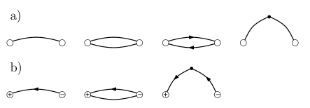
Figure 3: Diagrams for the calculation of the expansions in equations a) (B) and b) (B). The diagrammatic rules are presented in Refs. Abragam and Goldman, 1982; Stinchcombe et al., 1963.

$$\langle\hat{I}^{z}_{1}\hat{I}^{z}_{i}\rangle \simeq(-\beta)(M^{0}_{2})^{2}u_{1i}+(-\beta)^{2}\frac{1}{2}(M^{0}_{3})^{2}(u_{1i})^{2}+$$

$$+ (-\beta)^{2}M^{0}_{3}(+-z)M^{0}_{3}(-+z)(\frac{v_{1i}}{2})^{2}+$$ (47)

$$+ (-\beta)^{2}(M^{0}_{2})^{3}\sum_{j}u_{1j}u_{ji},$$

$$\langle\hat{I}^{+}_{1}\hat{I}^{-}_{i}\rangle \simeq(-\beta)\frac{v_{1i}}{2}M^{0}_{2}(+-)M^{0}_{2}(-+)+(-\beta)^{2}\frac{v_{1i}}{2}u_{1i}\frac{1}{2}[M^{0}_{3}(+z-)M^{0}_{3}(-z+)+M^{0}_{3}(z+-)M^{0}_{3}(z-+)]+$$

$$+ (-\beta)^{2}\sum_{j}\frac{v_{1j}}{2}\frac{v_{ji}}{2}M^{0}_{2}(+-)M^{0}_{2}(-+)\frac{1}{2}[M^{0}_{2}(+-)+M^{0}_{2}(-+)].$$ (48)

The final result can be expressed in terms of the following quantities, which depend on the particular lattice and the orientation of the magnetic field:

$$I_{2} =\sum_{i}(u_{1i})^{2},$$ (49a)

$$I_{3} =\sum_{i}(u_{1i})^{3},$$ (49b)

$$K_{3} =\sum_{i,j}u_{1i}u_{ij}u_{j1}.$$ (49c)

For the case of an fcc lattice, with the magnetic field parallel to the (111) crystalline direction, we obtain the values

$$I_{2} =1.6908\left(\frac{\mu_{0}}{4\pi}\frac{\hbar^{2}\gamma^{2}}{a^{3}}\right)^{2},$$ (50a)

$$I_{3} =-0.0072073\left(\frac{\mu_{0}}{4\pi}\frac{\hbar^{2}\gamma^{2}}{a^{3}}\right)^{3},$$ (50b)

$$K_{3} =2.1173\left(\frac{\mu_{0}}{4\pi}\frac{\hbar^{2}\gamma^{2}}{a^{3}}\right)^{3},$$ (50c)

where $2a$ is the edge of the conventional cubic cell. We refer to these values in Sec. III.3.

With these definitions, we have the following expansion for the dipolar interaction energy:

$$\frac{1}{N}\langle\mathcal{\hat{H}}^{\prime}_{D}\rangle=\beta G_{1}(t^{(1)}(\eta),t^{(2)}(\eta))+\\ \beta^{2}G_{2}(t^{(1)}(\eta),t^{(2)}(\eta),t^{(3)}(\eta))+\ldots;$$ (51)

for $v_{ij}=-\frac{1}{2}u_{ij}$, the functions $G_{1}$, and $G_{2}$ take the form

$$G_{1}\left(t^{(1)}(\eta),t^{(2)}(\eta)\right)=-\frac{1}{2}\left[(M^{0}_{2})^{2}I_{2}+\frac{1}{8}M^{0}_{2}(+-)M^{0}_{2}(-+)I_{2}\right]$$ (52a)

$$G_{2}\left(t^{(1)}(\eta),t^{(2)}(\eta),t^{(3)}(\eta)\right)=\frac{1}{2}\Bigl{[}\frac{1}{2}(M^{0}_{3})^{2}I_{3}+\frac{1}{16}M^{0}_{3}(+-z)M^{0}_{3}(-+z)I_{3}+(M^{0}_{2})^{3}K_{3}+$$

$$+\frac{1}{16}\left(M^{0}_{3}(+z-)M^{0}_{3}(-z+)+M^{0}_{3}(z+-)M^{0}_{3}(z-+)\right)I_{3}-\frac{1}{64}M^{0}_{2}(+-)M^{0}_{2}(-+)\left(M^{0}_{2}(+-)+M^{0}_{2}(-+)\right)K_{3}\Bigr{]}.$$ (52b)

References

- Greiner et al. (2002) M. Greiner, O. Mandel, T. Esslinger, T. W. Hänsch, and I. Bloch, Nature 415, 39 (2002).
- García-Ripoll et al. (2004) J. J. García-Ripoll, M. A. Martin-Delgado, and J. I. Cirac, Phys. Rev. Lett. 93, 250405 (2004).
- Stanley (1987) H. E. Stanley, Introduction to phase transitions and critical phenomena (Oxford University Press, New York, 1987).
- Auerbach (1998) A. Auerbach, Interacting electrons and quantum magnetism (Springer, New York, 1998).
- Landau and Binder (2005) D. P. Landau and K. Binder, A guide to Monte Carlo simulations in statistical physics (Cambridge University Press, Cambridge, 2005), 2nd ed.
- Ramanathan et al. (2004) C. Ramanathan, N. Boulant, Z. Chen, D. G. Cory, I. Chuang, and M. Steffen, Quantum Information Processing 3, 15 (2004).
- Abragam (2004) A. Abragam, Principles of nuclear magnetic resonance (Oxford Science publications / Oxford University Press, Oxford, 2004).
- Meier and Zakharchenya (1984) F. Meier and B. P. Zakharchenya, eds., Optical Orientation (North-Holland, Amsterdam, 1984).
- Tycko and Reimer (1996) R. Tycko and J. A. Reimer, J. Phys. Chem. 100, 13240 (1996).
- Abragam and Proctor (1958) A. Abragam and W. G. Proctor, Phys. Rev. 109, 1441 (1958).
- Goldman (1970) M. Goldman, Spin temperature and nuclear magnetic resonance in solids (Oxford Science Publications / Clarendon Press, Oxford, 1970).
- Michal and Tycko (1999) C. A. Michal and R. Tycko, Phys. Rev. B 60, 8672 (1999).
- Goto et al. (2004) A. Goto, K. Hashi, T. Shimizu, R. Miyabe, X. Wen, S. Ohki, S. Machida, T. Iijima, and G. Kido, Phys. Rev. B 69, 075215 (2004).
- Slichter (1990) C. P. Slichter, Principles of Magnetic Resonance (Springer-Verlag, 1990), 3rd ed.
- Oja and Lounasmaa (1997) A. S. Oja and O. V. Lounasmaa, Rev. Mod. Phys. 69, 1 (1997).
- Haeberlen (1976) U. Haeberlen, High resolution NMR in solids: Selective averaging (Academic Press, New York, 1976).
- Goldman et al. (1974) M. Goldman, M. Chapellier, V. H. Chau, and A. Abragam, Phys. Rev. B 10, 226 (1974).
- Mouritsen and Jensen (1980) O. G. Mouritsen and S. J. K. Jensen, Phys. Rev. B 22, 1127 (1980).
- Chapellier et al. (1970) M. Chapellier, M. Goldman, V. H. Chau, and A. Abragam, J. Appl. Phys. 41, 849 (1970).
- Quiroga et al. (1983a) L. Quiroga, J. Virlet, and M. Goldman, J. Magn. Reson. (1969) 51, 540 (1983a).
- Quiroga et al. (1983b) L. Quiroga, J. Virlet, and M. Goldman, J. Magn. Reson. (1969) 54, 161 (1983b).
- Abragam and Goldman (1982) A. Abragam and M. Goldman, Nuclear magnetism: order and disorder (Oxford Science Publications / Clarendon Press, Oxford, 1982).
- Goldman et al. (1975) M. Goldman, J. F. Jacquinot, M. Chapellier, and V. H. Chau, J. Magn. Reson. 18, 22 (1975).
- Stinchcombe et al. (1963) R. B. Stinchcombe, G. Horwitz, F. Englert, and R. Brout, Phys. Rev. 130, 155 (1963).
- Izyumov and Skryabin (1988) Y. A. Izyumov and Y. N. Skryabin, Statistical mechanics of magnetically ordered systems (Consultants Bureau, New York, 1988), translated from Russian.
- Wick (1950) G. C. Wick, Phys. Rev. 80, 268 (1950).
- Haldane (1983a) F. D. M. Haldane, Phys. Lett. A 93, 464 (1983a).
- Haldane (1983b) F. D. M. Haldane, Phys. Rev. Lett. 50, 1153 (1983b).
- Waugh et al. (1968) J. S. Waugh, L. M. Huber, and U. Haeberlen, Phys. Rev. Lett. 20, 180 (1968).
- Haeberlen and Waugh (1968) U. Haeberlen and J. S. Waugh, Phys. Rev. 175, 453 (1968).
- Mansfield (1971) P. Mansfield, J. Phys. C 4, 1444 (1971).
- Rhim et al. (1973a) W.-K. Rhim, D. D. Elleman, and R. W. Vaughan, J. Chem. Phys. 58, 1772 (1973a).
- Rhim et al. (1973b) W.-K. Rhim, D. D. Elleman, and R. W. Vaughan, J. Chem. Phys. 59, 3740 (1973b).
- Dyakonov and Perel (1974) M. I. Dyakonov and V. I. Perel, Sov. Phys. JETP 38, 177 (1974).
- Dyakonov and Perel (1984) M. I. Dyakonov and V. I. Perel, in Optical Orientation, edited by F. Meier and B. P. Zakharchenya (North-Holland, Amsterdam, 1984).
- Tomaselli et al. (1998) M. Tomaselli, D. deGraw, J. L. Yarger, M. P. Augustine, and A. Pines, Phys. Rev. B 58, 8627 (1998).
- Iijima et al. (2006) T. Iijima, K. Hashi, A. Goto, T. Shimizu, and S. Ohki, Chem. Phys. Lett. 419, 28 (2006).
- Goldman et al. (1968) M. Goldman, M. Chapellier, and V. H. Chau, Phys. Rev. 168, 301 (1968).