Local unitary versus local Clifford equivalence of stabilizer and graph states

Abstract

The equivalence of stabilizer states under local transformations is of fundamental interest in understanding properties and uses of entanglement. Two stabilizer states are equivalent under the usual stochastic local operations and classical communication criterion if and only if they are equivalent under local unitary (LU) operations. More surprisingly, under certain conditions, two LU equivalent stabilizer states are also equivalent under local Clifford (LC) operations, as was shown by Van den Nest et al. [Phys. Rev. A71, 062323]. Here, we broaden the class of stabilizer states for which LU equivalence implies LC equivalence ($LU\Leftrightarrow LC$) to include all stabilizer states represented by graphs with neither cycles of length $3$ nor $4$. To compare our result with Van den Nest et al.’s, we show that any stabilizer state of distance $\delta=2$ is beyond their criterion. We then further prove that $LU\Leftrightarrow LC$ holds for a more general class of stabilizer states of $\delta=2$. We also explicitly construct graphs representing $\delta>2$ stabilizer states which are beyond their criterion: we identify all $58$ graphs with up to $11$ vertices and construct graphs with $2^{m}-1$ ($m\geq 4$) vertices using quantum error correcting codes which have non-Clifford transversal gates.

I Introduction

Quantum entanglement, a phenomenon that has no counterpart in the classical realm, is widely recognized as an important resource in quantum computing and quantum information theoryNielsen . Stabilizer states form a particularly interesting class of multipartite entangled states, which play important roles in areas as diverse as quantum error correctionGottesman , measurement-based quantum computing, and cryptographic protocolsHans1 ; Hans2 ; Hans3 ; Hans4 . A stabilizer state on $n$ qubits is defined as the common eigenstate of its stabilizer: a maximally abelian subgroup of the $n$-qubit Pauli group $\mathcal{P}_{n}$ generated by the tensor products of the Pauli matrices and the identityGottesman . Recently, a special subset of stabilizer states (known as graph states due to their association with mathematical graphs) has become the subject of intensive study, and has proven to be useful in several fields of quantum information theoryHans4 ; Werner .

Despite their importance in quantum information science, multipartite entangled states are still far from being well understoodNielsen . The study of multipartite entanglement has usually focused on determining the equivalence classes of entangled states under local operations, but there are too many such equivalence classes under local unitary (LU) operations for a direct classification to be practical. The most commonly studied set of local operations are the invertible stochastic local operations assisted with classical communication (SLOCC), which yield a much smaller number of equivalence classes. For example, for three qubits, there are only two classes of fully entangled states under SLOCC, while $5$ real parameters are needed to specify the equivalence classes under LU operationsVidal ; Acin . However, the number of parameters needed to specify the equivalence classes under SLOCC grows exponentially with $n$, where $n$ is the number of qubits, so that specifying the equivalence classes for all states rapidly becomes impractical for $n\geq 4$Verstra .

For stabilizer states, a more tractable set of operations to study is the local Clifford (LC) group, which consists of the local unitary operations that map the Pauli group to itself under conjugation. In addition to forming a smaller class of operations, the local Clifford group has the additional advantage that the transformation of stabilizer states under LC operations can be reduced to linear algebra in a binary framework, which greatly simplifies all the necessary computationsHans4 .

It has been conjectured that any two stabilizer states which are LU equivalent are also LC equivalent (i.e. $LU\Leftrightarrow LC$ holds for every stabilizer state). If this were true, all of the advantages of working with the local Clifford group would be preserved when studying equivalences under an arbitrary local unitary operation. Due to its far-reaching consequences, proving that the $LU\Leftrightarrow LC$ equivalence holds for all stabilizer states is possibly one of the most important open problems in quantum information theory.

Graph states may prove to play a pivotal role in the proof of this conjecture, as it has been shown that every stabilizer state is LC equivalent to some graph stateMoor1 . Therefore, if it could be shown that $LU\Leftrightarrow LC$ holds for all graph states, it would follow that $LU\Leftrightarrow LC$ holds for all stabilizer states as well. Furthermore, it has been shown that an LC operation acting on a graph state can be realized as a simple local transformation of the corresponding graph, and that the orbits of graphs under such local transformations can be calculated efficientlyMoor1 ; DANIELSEN ; Moor2 . These results indicate that if the $LU\Leftrightarrow LC$ equivalence holds for all graph states, any questions concerning stabilizer states could be restated in purely graph theoretic terms. This would make it possible to use tools from graph theory and combinatorics to study the entanglement properties of stabilizer states, and to tackle problems which may have been too difficult to solve using more traditional approaches.

An important step towards a proof has been taken by Van den Nest et al.Moor3 , who have shown that two LU equivalent stabilizer states are also equivalent under LC operations if they satisfy a certain condition, known as the Minimal Support Condition (MSC), which ensures that their stabilizers possess some sufficiently rich structure. They also conjecture that states which do not satisfy the MSC will be rare, and therefore difficult to find.

In this paper, we seek to make some progress towards a proof of the $LU\Leftrightarrow LC$ conjecture, by proving that the $LU\Leftrightarrow LC$ equivalence holds for all stabilizer states whose corresponding graphs contain neither cycles of length $3$ nor $4$. We also give some results complementary to those of Van den Nest et al., by proving that the MSC does not hold for stabilizer states of distance $\delta=2$, and by explicitly constructing states of distance $\delta>2$ which also fail to satisfy the MSC. Our classification of stabilizer states is summarized in Fig. 1, which illustrates the relationship between the subsets covered by our results and those of Van den Nest et al., as well as those states for which the $LU\Leftrightarrow LC$ equivalence remains open.

Our paper is organized as follows: we first present some background information on graph states and stabilizers in Sec. II. In Sec. III we prove our Main Theorem, which states that $LU\Leftrightarrow LC$ holds for any graph state (and hence, any stabilizer state) whose corresponding graph contains neither cycles of length $3$ nor $4$. We go on to prove that all stabilizer states with distance $\delta=2$ fail to satisfy the MSC, whereas all stabilizer states with $\delta>2$ which satisfy the hypotheses of our Main Theorem do satisfy the MSC. We conclude Sec. III by using the proof of our Main Theorem to show that $LU\Leftrightarrow LC$ still holds for a particular subset of stabilizer states with $\delta=2$. In Sec. IV, we provide explicit examples of stabilizer states with distance $\delta>2$ which fail to satisfy the MSC: we identify all $58$ graphs of up to $11$ vertices which do not meet this condition, and construct two other series of graphs beyond the MSC for $n=2^{m}-1$ $(m\geq 4)$ from quantum error correcting codes with non-Clifford transversal gates. We conclude in Sec. V.

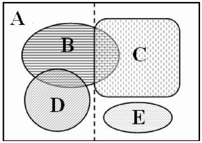
Figure 1: Relations between theorems presented in this paper. A: all graph states (there is a dashed line in the middle of A: the area left of the line are graphs of distance $\delta=2$ and the right area of the line are $\delta>2$ graphs); B: $LU\Leftrightarrow LC$ graphs given by Main Theorem; C: $LU\Leftrightarrow LC$ graphs given by Van den Nest et al.’s criterion; D: $LU\Leftrightarrow LC$ graphs of $\delta=2$ given by Theorem 2; E: Examples of $\delta>2$ graphs beyond the MSC, given in Sec. IV, whose $LU\Leftrightarrow LC$ equivalence remains open.

II Preliminaries

Before presenting our Main Theorem, we state some preliminaries in this section. We discuss the stabilizer formalism and graph states in Sec. IIA. Then in Sec. IIB we introduce the concept of minimal supports and Van den Nest et al.’s criterion.

II.1 Stabilizers states and graph states

The $n$-qubit Pauli group ${\mathcal{P}}_{n}$ consists of all $4\times 4^{n}$ local operators of the form $R=\alpha_{R}R_{1}\otimes\dots\otimes R_{n}$, where $\alpha_{R}\in\{\pm 1,\pm i\}$ is an overall phase factor and $R_{i}$ is either the $2\times 2$ identity matrix $I$ or one of the Pauli matrices $X$, $Y$, or $Z$. We can write $R$ as $\alpha_{R}(R_{1})_{1}(R_{2})_{2}\dots(R_{n})_{n}$ or $\alpha_{R}R_{1}R_{2}\dots R_{n}$ when it is clear what the qubit labels are. The $n$-qubit Clifford group ${\mathcal{L}}_{n}$ is the group of $n\times n$ unitary matrices that map ${\mathcal{P}}_{n}$ to itself under conjugation.

A stabilizer ${\mathcal{S}}$ in the Pauli group ${\mathcal{P}}_{n}$ is defined as an abelian subgroup of ${\mathcal{P}}_{n}$ which does not contain $-I$. A stabilizer consists of $2^{m}$ Hermitian Pauli operators for some $m\leq n$. As the operators in a stabilizer commute with each other, they can be diagonalized simultaneously and moreover, if $m=n$, then there exists a unique state $|\psi\rangle$ on $n$ qubits such that $R|\psi\rangle=|\psi\rangle$ for every $R\in{\mathcal{S}}$. Such a state $|\psi\rangle$ is called the stabilizer state and the group ${\mathcal{S}}={\mathcal{S}}(|\psi\rangle)$ is called the stabilizer of $|\psi\rangle$. A stabilizer state can also be viewed as a self-dual code over $GF(4)$ under the trace inner productDANIELSEN . The distance $\delta$ of the state is the weight of the minimum weight element in $\mathcal{S}(|\psi\rangle)$DANIELSEN .

Two $n$-qubit states $|\psi\rangle$ and $|\psi^{\prime}\rangle$ are said to be local unitary (LU) equivalent if there exists an LU operation

$$\mathcal{U}_{n}=\bigotimes\limits_{i=1}^{n}U_{i}$$ (1)

which maps $|\psi^{\prime}\rangle$ to $|\psi\rangle$.

Two $n$-qubit states $|\psi\rangle$ and $|\psi^{\prime}\rangle$ are said to be local Clifford (LC) equivalent if there exists an LU operation in the Clifford group

$$\mathcal{K}_{n}=\bigotimes\limits_{i=1}^{n}K_{i}$$ (2)

which maps $|\psi^{\prime}\rangle$ to $|\psi\rangle$, where $K_{i}\in\mathcal{L}_{1}$ for $i=1,\ldots,n$.

Throughout the paper we will use $\mathcal{U}_{n}$ and $\mathcal{K}_{n}$ to denote operations of the form Eq. (1) and (2), respectively.

Graph states are a special kind of stabilizer state associated with graphsHans4 . A graph $G$ consists of two types of elements, namely vertices ($V$) and edges ($E$). Every edge has two endpoints in the set of vertices, and is said to connect or join the two endpoints. The degree of a vertex is the number of edges ending at that vertex. A path in a graph is a sequence of vertices such that from each vertex in the sequence there is an edge to the next vertex in the sequence. A cycle is a path such that the start vertex and end vertex are the same. The length of a cycle is the number of edges that the cycle has.

For every graph $G$ with $n$ vertices, there are $n$ operators $R_{a}^{G}\in\mathcal{P}_{n}$ for $a=1,2,\ldots,n$ defined by

$$R_{a}^{G}=X_{a}\bigotimes_{\{a,b\}\in E}Z_{b},$$ (3)

It is straightforward to show that any two $R_{a}^{G}$s commute, hence the group generated by $\{R_{a}^{G}\}_{a=1}^{n}$ is a stabilizer group $\mathcal{S}$ and stabilizes a unique state $|\psi_{G}\rangle$. We call each $R_{a}^{G}$ the standard generator associated with vertex $a$ of graph $G$. Throughout the paper we use $|\psi_{G}\rangle$ to denote the unique state corresponding to a given graph $G$.

Any stabilizer state is local Clifford (LC) equivalent to some graph statesMoor1 . Thus, it suffices to prove $LU\Leftrightarrow LC$ for all graph states in order to show that $LU\Leftrightarrow LC$ for all stabilizer states.

II.2 Minimal supports

The support $supp(R)$ of an element $R\in{\mathcal{S}}(|\psi\rangle)$ is the set of all $i\in\{1,...,n\}$ such that $R_{i}$ differs from the identity. Let $\omega=\{i_{1},\dots,i_{k}\}$ be a subset of $\{1,\dots,n\}$. Tracing out all qubits of $|\psi\rangle$ outside $\omega$ gives the mixed state

$$\rho_{\omega}(\psi)=\frac{1}{2^{|\omega|}}\sum_{R\in{\mathcal{S}}(|\psi\rangle),supp(R)\subseteq\omega}R\,.$$ (4)

Using the notation $U_{\omega}=U_{i_{1}}\otimes\ldots\otimes U_{i_{k}}$, it follows from $\mathcal{U}_{n}|\psi^{\prime}\rangle=|\psi\rangle$ that

$$U_{\omega}\rho_{\omega}(\psi^{\prime})U_{\omega}^{\dagger}=\rho_{\omega}(\psi)\,.$$ (5)

A minimal support of ${\mathcal{S}}(|\psi\rangle)$ is a set $\omega\subseteq\{1,...,n\}$ such that there exists an element in ${\mathcal{S}}(|\psi\rangle)$ with support $\omega$, but there exist no elements with support strictly contained in $\omega$. An element in ${\mathcal{S}}(|\psi\rangle)$ with minimal support is called a minimal element. We denote by $A_{\omega}(|\psi\rangle)$ the number of elements $R\in{\mathcal{S}}(|\psi\rangle)$ with $supp(R)=\omega$. Note that $A_{\omega}(|\psi\rangle)$ is invariant under LU operationsMoor3 . We use $\mathcal{M}(|\psi\rangle)$ to denote the subgroup of ${\mathcal{S}}(|\psi\rangle)$ generated by all the minimal elements. The following Lemma 1 is given in Moor3 .

[Lemma 1]: Let $|\psi\rangle$ be a stabilizer state and let $\omega$ be a minimal support of ${\mathcal{S}}(|\psi\rangle)$. Then $A_{\omega}(|\psi\rangle)$ is equal to 1 or 3 and the latter case can only occur if $|\omega|$ is even.

If $\omega$ is a minimal support of ${\mathcal{S}}(|\psi\rangle)$, it follows from the proof of Lemma 1 in Moor3 that the minimal elements with support $\omega$, up to an LC operation, must have one of the following two forms:

$$A_{\omega}(|\psi\rangle)=1\ : \ Z^{\otimes\omega}$$

$$A_{\omega}(|\psi\rangle)=3\ : \ \{X^{\otimes\omega},(-1)^{(|\omega|/2)}Y^{\otimes\omega},Z^{\otimes\omega}\}\,.$$ (6)

Eqs.(4), (5) and (6) directly lead to the following Fact 1, which was originally proved by Rains in Rains :

[Fact 1]: If $|\psi^{\prime}\rangle$ and $|\psi\rangle$ are LU equivalent stabilizer states, i.e. $\mathcal{U}_{n}|\psi^{\prime}\rangle=|\psi\rangle$, then for each minimal support $\omega$, the equivalence $\mathcal{U}_{n}$ must take the group generated by all the minimal elements of support $\omega$ in $\mathcal{S}(|\psi^{\prime}\rangle)$ to the corresponding group generated by all the minimal elements of support $\omega$ in $\mathcal{S}(|\psi\rangle)$.

Based on the above Fact 1, the following Theorem 1 was proven in Moor3 as their main result:

[Theorem 1]: Let $|\psi\rangle$ be a fully entangled stabilizer state for which all three Pauli matrices $X,Y,Z$ occur on every qubit in $\mathcal{M}(|\psi\rangle)$. Then every stabilizer state $|\psi^{\prime}\rangle$ which is LU equivalent to $|\psi\rangle$ must also be LC equivalent to $|\psi\rangle$.

The condition given in Theorem 1, that all three Pauli matrices $X,Y,Z$ occur on every qubit in $\mathcal{M}(|\psi\rangle)$, is called the minimal support condition (MSC).

For any LU operation $\mathcal{U}_{n}=\bigotimes\limits_{i=1}^{n}U_{i}$ which maps another stabilizer state $|\psi^{\prime}\rangle$ to the stabilizer state $|\psi\rangle$, the proof of Theorem 1 further specifies the following

[Fact 2]: If all three Pauli matrices $X,Y,Z$ occur on the $j$th qubit in $\mathcal{M}(|\psi\rangle)$, then $U_{j}$ must be a Clifford operation. Therefore, if the MSC condition is satisfied for $|\psi\rangle$, then $\mathcal{U}_{n}$ must be an LC operation.

In Moor3 it is also shown that although $n$-GHZ statesGHZ do not possess this structure, $LU\Leftrightarrow LC$ still holds.

III The main theorem

We now present the new criterion we have found for the $LU\Leftrightarrow LC$ equivalence of graph states. Sec. IIIA, IIIB, IIIC, and IIID are devoted to proving the main result of the paper. An algorithm for constructing the LC operation $\mathcal{K}_{n}=\bigotimes\limits_{i=1}^{n}K_{i}$, where $K_{i}\in\mathcal{L}_{1}$ for any $i$, is given in Sec. IIIE and Theorem 2, which covers additional $LU\Leftrightarrow LC$ equivalences for $\delta=2$ graphs beyond the main theorem, is given in Sec. IIIF.

The main result of the paper is the following:

[Main Theorem]: $LU\Leftrightarrow LC$ equivalence holds for any graph $G$ with neither cycles of length 3 nor 4.

[Proof]: In order to prove that $LU\Leftrightarrow LC$ holds for $|\psi_{G}\rangle$, we will show that for any stabilizer state $|{\psi}_{G}^{\prime}\rangle$ satisfying $\mathcal{U}_{n}|{\psi}_{G}^{\prime}\rangle=|{\psi}_{G}\rangle$, there exists an LC operation $\mathcal{K}_{n}$ such that $\mathcal{K}_{n}|{\psi}_{G}^{\prime}\rangle=|{\psi}_{G}\rangle$. The proof is presented in several sections below, ending in Sec. IIID on page 9.

We prove this theorem constructively, i.e. we construct $\mathcal{K}_{n}$ explicitly from the given $\mathcal{U}_{n}$, $|\psi_{G}\rangle$, and $|\psi^{\prime}_{G}\rangle$. Before giving the details of our proof, we give a brief outline of our strategy. We will assume that throughout our proof that all graphs have neither cycles of length $3$ nor $4$.

First, we show that any graph of distance $\delta>2$ satisfies the MSC, hence $LU\Leftrightarrow LC$ holds for them. However, we will also show that any graph of distance $\delta=2$ is beyond the MSC. Therefore, we only need to prove the Main Theorem for $\delta=2$ graphs.

We then partition the vertex set $V(G)$ of graph $G$ into subsets $\{V_{1}(G),V_{2}(G),V_{3}(G),V_{4}(G)\}$ as defined later. We show that for all vertices $v\in V_{3}(G)\cup V_{4}(G)$, the operator $U_{v}$ in $\mathcal{U}_{n}$ must be a Clifford operation, i.e. $U_{v}\in\mathcal{L}_{1}$. For vertices $v\in V_{1}(G)\cup V_{2}(G)$, we will give a procedure, called the standard procedure, for constructing $K_{v}$. In effect, this corresponds to an “encoding” of any vertex $v\in V_{2}$ and all the degree one vertices $w\in V_{1}$ to which $v$ is connected into a repetition code (i.e. “deleting” the degree one vertices from $G$), and then a “decoding” of the code.

We illustrate the proof idea in Fig. 2. Due to some technical reasons, we first show $U_{v}\in\mathcal{L}_{1}$ for all $v\in V_{4}$ in Sec. IIIA. Then we give the standard procedure in Sec. IIIB. We use an example to show explicitly how the procedure works, with explanations of why this procedure actually works in general. Finally, in Sec. IIIC we show that $U_{v}\in\mathcal{L}_{1}$ for all $v\in V_{3}(G)\cup V_{4}(G)$, and construct $K_{v}$ for all $v\in V_{1}(G)\cup V_{2}(G)$ from the standard procedure.

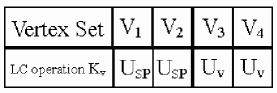
Figure 2: An illustration of the construction of $\mathcal{K}_{n}$: we will simply choose $K_{v}=U_{v}$ for all $v\in V_{3}\cup V_{4}$, and use the standard procedure(SP) to construct $K_{v}=U_{SP}$ for all $v\in V_{1}\cup V_{2}$.

The four types of vertices we use for a graph $G$ are defined as follows. $V_{1}(G)$ is the degree one vertices of $G$. $V_{2}(G)$ is the set of vertices $V_{2}(G)=\{v|v$ connects to some $w\in V_{1}(G)\}$. The set $V_{3}(G)$ is given by $V_{3}(G)=\{v|v$ not in $V_{1}(G)$, and $v$ only connects to $w\in V_{2}(G)\}$. Finally, the set $V_{4}(G)$ is defined by $V_{4}(G)=V(G)\setminus(V_{1}(G)\cup V_{2}(G)\cup V_{3}(G))$. For convenience, we also apply this partitioning of vertices to $\delta>2$ graphs, hence $V(G)=V_{4}(G)$. Fig. 3 gives an example of such partitions.

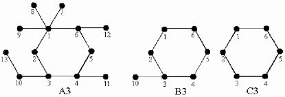
Figure 3: Examples of the partition: $V_{1}(A3)=\{7,8,9,11,12,13\}$, $V_{2}(A3)=\{1,4,6,10\}$, $V_{3}(A3)=\{5\}$ and $V_{4}(A3)=\{2,3\}$; $V_{1}(B3)=\{10\}$, $V_{2}(B3)=\{3\}$, $V_{3}(B3)=\emptyset$ and $V_{4}(B3)=\{1,2,4,5,6\}$; $C3$ is a graph of $\delta=3$ hence $V_{1}(C3)=V_{2}(C3)=V_{3}(C3)=\emptyset$, and $V_{4}(C3)=V(C3)=\{1,2,3,4,5,6\}$.

III.1 $\delta>2$ and $\delta=2$ graphs and Case $V_{4}$

We first provide some lemmas which lead to a proof of the Main Theorem for $\delta>2$ graphs. Then we show that all $\delta=2$ graphs are beyond the MSC.

III.1.1 $\delta>2$ graphs

[Lemma 2]: For a vertex $v\in V(G)$ which is unconnected to any degree one vertex, if it is neither in cycles of length $3$ nor $4$, and then $R_{v}$ is the only minimal element of support $supp(R_{v})$.

[Proof]: Suppose the vertex $v$ connects to vertices $i_{1},i_{2},\cdots i_{k},$, then $R_{v}=X_{v}Z_{i_{1}}Z_{i_{2}}\cdots Z_{i_{k}}$. If there exists an element $S_{m}\in\mathcal{S}(|\psi_{G}\rangle)$ such that $supp(S_{m})\subseteq supp(R_{v})$, then $S_{m}$ must be expressed as a product of elements in $\{R_{v},R_{i_{1}},R_{i_{2}},\cdots R_{i_{k}}\}$. However since $v$ is neither in any cycle of length $3$ nor $4$, then any product of elements in $\{R_{v},R_{i_{1}},R_{i_{2}},\cdots R_{i_{k}}\}$ (except $R_{v}$ itself) must contain at least one Pauli operator $\alpha_{j}$ acting on the $j$th qubit where $j$ is not in $supp(R_{v})$. $\square$

This directly leads to the following Lemma 3 for $\delta>2$ graphs:

[Lemma 3]: For any graph $G$ with $\delta>2$, if there are neither cycles of length $3$ nor $4$, then $G$ satisfies the MSC, and hence $LU\Leftrightarrow LC$ holds for $G$.

[Proof]: Since $\delta>2$, then all vertices $v\in V(G)$ are unconnected to any degree one vertices. Then by Lemma 2, $\mathcal{M}(|\psi\rangle)=\mathcal{S}(|\psi\rangle)$, and therefore the MSC is satisfied. $\square$

Lemma 2 tells us that for any vertex $v\in V_{4}(G)$, we must have $U_{v}\in\mathcal{L}_{1}$, according to Fact 2. Lemma 3 shows that we only need to prove the Main Theorem for graphs of $\delta=2$.

III.1.2 $\delta=2$ graphs

[Proposition 1]: Stabilizer states with distance $\delta=2$ are beyond the MSC.

[Proof]: A stabilizer state $|\psi\rangle$ with $\delta=2$ has at least one weight two element in its stabilizer $\mathcal{S}(|\psi\rangle)$. We denote one such weight two element by $\alpha_{i}\beta_{k}$, where $\alpha_{j}$ and $\beta_{k}$ are one of the three Pauli operators $X,Y,Z$ on the $j$th and $k$th qubits respectively, up to an overall phase factor of $\pm 1$ or $\pm i$. Now consider any element $R$ in $\mathcal{S}(|\psi\rangle)$ with a support $\omega$ such that $\omega\cap\{j,k\}\neq\emptyset$. We can write $R$ in the form $R_{1}R_{2}\cdots R_{n}$ where each $R_{i}$ is either the identity matrix $I$ or one of the Pauli matrices $X,Y,Z$, up to an overall phase factor of $\pm 1$ or $\pm i$. Then there are three possibilities: (i) If $\omega\cap\{j,k\}$ is $\{j\}$ or $\{k\}$, then since $R$ commutes with $\alpha_{j}\beta_{k}$, the operator $R_{j}$ ($R_{k}$) can only be $\alpha_{j}$ ($\beta_{k}$), up to an overall phase factor of $\pm 1$ or $\pm i$. (ii) If $\omega=\{j,k\}$, then since $R$ commutes with $\alpha_{j}\beta_{k}$, we either have $R_{j}R_{k}=\alpha_{j}^{\prime}\beta_{k}^{\prime}$, where $\alpha_{j}^{\prime}$ anticommutes with $\alpha_{j}$ and $\beta_{k}^{\prime}$ anticommutes with $\beta_{k}$, or $R_{j}R_{k}=\alpha_{j}\beta_{k}$. The former is impossible, as the whole graph is connected, so the latter must hold. (iii) If $\omega$ strictly contains $\{j,k\}$, then $R$ is not a minimal element. It follows that in $\mathcal{M}(|\psi\rangle)$, only $\alpha_{j}$ appears on the $j$th qubit and only $\beta_{k}$ appears on the $k$th qubit, showing that $\mathcal{S}(|\psi\rangle)$ is beyond the MSC.$\square$

Furthermore, the local unitary operation $\mathcal{U}_{n}$ which maps another $\delta=2$ stabilizer state $|\psi^{\prime}\rangle$ to $|\psi\rangle$ is not necessarily in the Clifford group, particularly on the $j$th and $k$th qubits. Note that it is always true for any angle $\theta$ that

$$\alpha_{j}(\theta)\beta_{k}(-\theta)|\psi\rangle=e^{i\alpha_{j}\theta}e^{-i\beta_{k}\theta}|\psi\rangle=|\psi\rangle.$$ (7)

To interpret Proposition 1 in view of graphs, it is noted that any fully connected graph $G$ with degree one vertices represents a graph state $|\psi_{G}\rangle$ of $\delta=2$. Therefore, a graph with degree one vertices is beyond the MSC. In particular, for a graph $G$ with neither cycles of length $3$ nor $4$, each weight two element in $\mathcal{S}(|\psi_{G}\rangle)$ corresponds to the standard generator of a degree one vertex in $G$.

III.2 Case $V_{1}\cup V_{2}$: The standard procedure

The main idea behind the standard procedure is to convert the $LU$-equivalent stabilizer states $|\psi_{G}\rangle$ and $|\psi^{\prime}_{G}\rangle$ into the corresponding (LC equivalent) canonical forms for which we can prove $LU\Leftrightarrow LC$ by applying “encoding” and “decoding” methods. We can then work backwards from those canonical forms to prove that $LU\Leftrightarrow LC$ for $|\psi_{G}\rangle$.

We use a simple example, as shown in graph B4 of Fig. 4, to demonstrate how the standard procedure works. The standard procedure decomposes into five steps. In each step, we also explain how the step works for the general case.

Figure 4: $A4$ is a subgraph of both $B4$ and $C4$.

Note that $|\psi_{A4}\rangle$ is a GHZ state; hence $LU\Leftrightarrow LC$ holds. The standard generator of the stabilizer for graph $A4$ is $\{XZI,ZXZ,IZX\}$. However, as we will see later in step 4, $LU\Leftrightarrow LC$ for $A4$ does not guarantee that $LU\Leftrightarrow LC$ for $B4$.

We now prove $LU\Leftrightarrow LC$ for $|\psi_{B4}\rangle$.

III.2.1 Step 1: Transform into a new basis by LC operation

It is straightforward to show

$$|\psi_{B4}\rangle=\frac{1}{2^{5/2}}\sum\limits_{a_{j}=0,1}(-1)^{f(E)}|a_{1}a_{2}a_{3}a_{4}a_{5}\rangle,$$ (8)

where $f(E)=a_{1}a_{2}+a_{2}a_{3}+a_{3}a_{4}+a_{3}a_{5}$, which is determined by the the edge set $E(B4)$.

Performing Hadamard transform on the fourth and fifth qubits, we get

$$|\tilde{\psi}_{B4}\rangle=H_{4}\otimes H_{5}|\psi_{B}\rangle=\frac{1}{\sqrt{2}}(|\xi_{0}\rangle|000\rangle+|\xi_{1}\rangle|111\rangle),$$ (9)

where

$$|\xi_{0}\rangle = \frac{1}{2}(|00\rangle+|01\rangle+|10\rangle-|11\rangle)$$

$$|\xi_{1}\rangle = \frac{1}{2}(|00\rangle-|01\rangle+|10\rangle+|11\rangle).$$ (10)

The form of $|\tilde{\psi}_{B4}\rangle$ in Eq.(9) is not hard to understand. By performing $H_{4}\otimes H_{5}$, the standard generator of $|\psi_{B4}\rangle$ will be transformed to $\{Z_{3}Z_{4},Z_{3}Z_{5}...\}$, hence only the terms of $|000\rangle$ and $|111\rangle$ appear on the qubits $3,4,5$. Furthermore, for the supports $\omega_{1}=(3,4),\omega_{2}=(3,5)$, we have $A_{\omega_{1}}(|\psi_{B4}\rangle)=A_{\omega_{2}}(|\psi_{B4}\rangle)=1$.

For any other stabilizer state which is LU equivalent to $|\psi_{B4}\rangle$, there exist an LU operation $\mathcal{U}_{5}$ such that $\mathcal{U}_{5}|\psi_{B4}^{\prime}\rangle=|\psi_{B4}\rangle$. According to Fact 1, for the supports $\omega_{1}=(3,4),\omega_{2}=(3,5)$, there must also be $A_{\omega_{1}}(|\psi_{B4}^{\prime}\rangle)=A_{\omega_{2}}(|\psi_{B4}^{\prime}\rangle)=1$. Suppose the corresponding minimal elements of $\omega_{1},\omega_{2}$ are $\alpha_{3}\beta_{4},\alpha_{3}\gamma_{5}$ respectively, then there exist $F_{3},F_{4},F_{5}\in\mathcal{L}_{1}$, such that $(F_{3}\alpha_{3}F_{3}^{\dagger})\otimes(F_{4}\beta_{4}F_{4}^{\dagger})=Z_{3}Z_{4}$, $(F_{3}\alpha_{3}F_{3}^{\dagger})\otimes(F_{5}\gamma_{5}F_{5}^{\dagger})=Z_{3}Z_{5}$. Therefore, we have

$$|\tilde{\psi}_{B}^{\prime}\rangle = F_{3}\otimes F_{4}\otimes F_{5}|\psi^{\prime}_{B}\rangle$$ (11)

$$= \frac{1}{\sqrt{2}}(|\chi_{0}\rangle|000\rangle+|\chi_{1}\rangle|111\rangle),$$

where $|\chi_{0}\rangle$ and $|\chi_{1}\rangle$ are two states of qubits $1$ and $2$.

The states $|\tilde{\psi}_{B}\rangle$ and $|\tilde{\psi}_{B}^{\prime}\rangle$ given in Eqs.(9,11) are then called canonical forms of $|{\psi}_{B}\rangle$ and $|{\psi}_{B}^{\prime}\rangle$, respectively.

Then we have

$$\tilde{\mathcal{U}}_{5}|\tilde{\psi}_{B}^{\prime}\rangle=|\tilde{\psi}_{B}\rangle,$$ (12)

where

$$\tilde{\mathcal{U}}_{5}=H_{4}\otimes H_{5}\mathcal{U}_{5}F_{3}^{\dagger}\otimes F_{4}^{\dagger}\otimes F_{5}^{\dagger}$$ (13)

i.e. $\tilde{U}_{1}=U_{1}$, $\tilde{U}_{2}=U_{2}$, $\tilde{U}_{3}=U_{3}F_{3}^{\dagger}$, $\tilde{U}_{4}=H_{4}U_{4}F_{4}^{\dagger}$, $\tilde{U}_{5}=H_{5}U_{5}F_{5}^{\dagger}$.

Eq.(12) is then our new starting point, since $|\psi^{\prime}_{B4}\rangle$ and $|\psi_{B4}\rangle$ are LC equivalent if and only if $|\tilde{\psi}^{\prime}_{B4}\rangle$ and $|\tilde{\psi}_{B}\rangle$ are LC equivalent, then we can always get the former when we prove the latter by reversing Eq. (13), as we will do from eqs. (35) to (36).

Note the procedure of getting Eq.(12) is general, i.e. we can always do the same thing for any $\delta=2$ graph state and its LU equivalent graph states. To be more precise, for a general graph $G$ of $n$ vertices, consider a vertex $a\in V_{2}(G)$, and let $N(a)$ be the set of all degree one vertices in $V(G)$ which connect to $a$. If the size of this set is $|N(a)|=k$, then without loss of generality we can rename the qubits so that the vertices $a$ and $b\in N(a)$ are represented by the last $k+1$ qubits of $|\psi_{G}\rangle$.

Applying the Hadamard transform $\tilde{H}_{a}=\bigotimes_{b\in N(a)}H_{b}$ to $|\psi_{G}\rangle$ gives a new stabilizer state $|\tilde{\psi}_{G}^{(a)}\rangle$ as shown below.

$$\tilde{H}_{a}|\psi_{G}\rangle = |\tilde{\psi}_{G}^{(a)}\rangle$$ (14)

$$= \frac{1}{\sqrt{2}}(|\xi_{0}\rangle|0\rangle^{\bigotimes(k+1)}+|\xi_{1}\rangle|1\rangle^{\bigotimes(k+1)}),$$

where $|\xi_{0}\rangle$ and $|\xi_{1}\rangle$ are two states of the other $n-(k+1)$ qubits.

Similarly, for any stabilizer state $|\psi^{\prime}_{G}\rangle$ which is LU equivalent to $|\psi_{G}\rangle$, i.e. $\mathcal{U}_{n}|\psi^{\prime}_{G}\rangle=|\psi_{G}\rangle$, there must exist $F_{a},F_{b}\in\mathcal{L}_{1}$ (for all $b\in N(a)$) such that

$$(F_{a}\alpha_{a}F_{a}^{\dagger})\otimes(F_{b}\beta_{b}F_{b}^{\dagger})=Z_{a}Z_{b},$$ (15)

for $\alpha_{a}\beta_{b}\in\mathcal{S}(|\psi^{\prime}_{G}\rangle)$.

Define $\tilde{F}_{a}=F_{a}\bigotimes_{b\in N(a)}F_{b}$, we have

$$\tilde{F}_{a}|\psi^{\prime}_{G}\rangle = |\tilde{\psi^{\prime}}_{G}^{(a)}\rangle$$ (16)

$$= \frac{1}{\sqrt{2}}(|\chi_{0}\rangle|0\rangle^{\bigotimes(k+1)}+|\chi_{1}\rangle|1\rangle^{\bigotimes(k+1)}),$$

where $|\chi_{0}\rangle$ and $|\chi_{1}\rangle$ are two states of the other $n-(k+1)$ qubits.

We apply the above procedure for all $a\in V_{2}(G)$. Define $\tilde{H}=\bigotimes_{a\in V_{2}(G)}{\tilde{H}_{a}}$ and $\tilde{F}=\bigotimes_{a\in V_{2}(G)}{\tilde{F}_{a}}$, we get

$$\tilde{H}|\psi_{G}\rangle = |\tilde{\psi}_{G}\rangle$$

$$\tilde{F}|\psi_{G}\rangle = |\tilde{\psi}_{G}^{\prime}\rangle,$$ (17)

Now define

$$\tilde{\mathcal{U}}_{n}=\bigotimes_{i=1}^{n}\tilde{U}_{i},$$ (18)

where $\tilde{U}_{i}=U_{i}$ for all $i\in V_{3}(G)\cup V_{4}(G)$, $\tilde{U}_{a}=U_{a}F_{a}^{\dagger}$ for all $a\in V_{2}(G)$, and $\tilde{U}_{b}=H_{b}U_{b}F_{b}^{\dagger}$ for all $b\in N(a)$. We then have $\tilde{\mathcal{U}}_{n}|\tilde{\psi}_{G}^{\prime}\rangle=|\tilde{\psi}_{G}\rangle$.

It can be seen that $|\psi_{G}^{\prime}\rangle$ and $|\psi_{G}\rangle$ are LC equivalent if and only if $|\tilde{\psi}_{G}^{\prime}\rangle$ and $|\tilde{\psi}_{G}\rangle$ are LC equivalent. Therefore, we can use the states $|\tilde{\psi}_{G}^{\prime}\rangle$ and $|\tilde{\psi}_{G}\rangle$ as our new starting point.

Our current situation is summarized in the following diagram.

$$\begin{CD}|\psi_{G}\rangle @<{\mathcal{U}_{n}=\bigotimes_{i=1}^{n}U_{i}}<{}<|\psi_{G}^{\prime}\rangle\\ @V{\tilde{H}=\bigotimes_{a\in V_{2}(G)}\tilde{H}_{a}}V{}V@V{}V{\tilde{F}=\bigotimes_{a\in V_{2}(G)}\tilde{F}_{a}}V\\ |\tilde{\psi}_{G}\rangle @<{\tilde{\mathcal{U}}_{n}=\bigotimes_{i=1}^{n}\tilde{U}_{i}}<{}<|\tilde{\psi}_{G}^{\prime}\rangle\\ \end{CD}$$

III.2.2 Step 2: Encode into repetition codes

Now we can encode the qubits $3,4,5$ into a single logical qubit, i.e. $|0_{L}\rangle=|000\rangle$, $|1_{L}\rangle=|111\rangle$. Define $|\bar{\psi}_{B4}\rangle=(|\xi_{0}\rangle|0_{L}\rangle+|\xi_{1}\rangle|1_{L}\rangle)$, and $|\bar{\psi}_{B4}^{\prime}\rangle=(|\chi_{0}\rangle|0_{L}\rangle\rangle+|\chi_{1}\rangle|1_{L}\rangle)$, then both $|\bar{\psi}_{B4}\rangle$ and $|\bar{\psi}_{B4}^{\prime}\rangle$ are $3$-qubit stabilizer states. Especially, $|\bar{\psi}_{B4}\rangle$ is exactly the graph state $|\psi_{A4}\rangle$ represented by graph $A4$. Now Eq.(12) becomes

$$\bar{\mathcal{U}_{3}}|\bar{\psi}_{B4}^{\prime}\rangle=|\bar{\psi}_{B4}\rangle,$$ (19)

where $\bar{\mathcal{U}_{3}}=U_{1}\otimes U_{2}\otimes U_{L}^{(3)}$, and $U_{L}^{(3)}$ is a logical operation acting on the logical qubit, which must be of some special forms as we discuss below. The upper index $(3)$ indicates that we may understand this logical qubit $L$ as being the $3$rd qubit in graph $A4$.

Due to Fact 1, we must have

$$\tilde{U}_{3}Z_{3}\tilde{U}_{3}^{\dagger}\otimes\tilde{U}_{4}Z_{4}\tilde{U}_{4}^{\dagger} = Z_{3}Z_{4}$$

$$\tilde{U}_{3}Z_{3}\tilde{U}_{3}^{\dagger}\otimes\tilde{U}_{5}Z_{5}\tilde{U}_{5}^{\dagger} = Z_{3}Z_{5}$$ (20)

which means either

$$\tilde{U}_{3}Z_{3}\tilde{U}_{3}^{\dagger} = Z_{3}$$

$$\tilde{U}_{4}Z_{4}\tilde{U}_{4}^{\dagger} = Z_{4}$$

$$\tilde{U}_{5}Z_{5}\tilde{U}_{5}^{\dagger} = Z_{5},$$ (21)

which gives $\tilde{U}_{3}=diag(1,e^{i\theta_{1}}),\tilde{U}_{4}=diag(1,e^{i\theta_{2}}),\tilde{U}_{5}=diag(1,e^{i\theta_{3}})$ for some $\theta_{1},\theta_{2},\theta_{3}$, or

$$\tilde{U}_{3}Z_{3}\tilde{U}_{3}^{\dagger} = -Z_{3}$$

$$\tilde{U}_{4}Z_{4}\tilde{U}_{4}^{\dagger} = -Z_{4}$$

$$\tilde{U}_{5}Z_{5}\tilde{U}_{5}^{\dagger} = -Z_{5}$$ (22)

which gives $\tilde{U}_{3}=diag(1,e^{i\theta_{1}})X_{3}$, $\tilde{U}_{4}=diag(1,e^{i\theta_{2}})X_{4}$, $\tilde{U}_{5}=diag(1,e^{i\theta_{3}})X_{5}$ for some $\theta_{1},\theta_{2},\theta_{3}$.

Therefore, we must have $U_{L}^{(3)}=diag(1,e^{i(\theta_{1}+\theta_{2}+\theta_{3})})$ if Eq.(21) holds, or $U_{L}^{(3)}=diag(1,e^{i(\theta_{1}+\theta_{2}+\theta_{3})})X_{L}^{(3)}$ if Eq.(22) holds.

Note the procedure of getting Eq.(19) and the result of the possible forms that $U_{L}$ possesses is also general. Recall that we have two states of the form given in Eq. (14) and Eq. (16), we can encode the qubits $a$ and $b\in N(a)$ into a single logical qubit, by writing $|0_{L}\rangle=|0\rangle^{\otimes(k+1)}$ and $|1_{L}\rangle=|1\rangle^{\otimes(k+1)}$. We can then define two new stabilizer states $|\bar{\psi}_{G}^{(a)}\rangle$ and $|\bar{\psi}_{G}^{\prime(a)}\rangle$, given by

$$|\bar{\psi}_{G}^{(a)}\rangle = |\xi_{0}\rangle|0_{L}\rangle+|\xi_{1}\rangle|1_{L}\rangle,$$

$$|\bar{\psi}_{G}^{\prime(a)}\rangle = |\chi_{0}\rangle|0_{L}\rangle+|\chi_{1}\rangle|1_{L}\rangle.$$ (23)

Both are stabilizer states of $m$ qubits, where $m=n-k$. In particular, $|\bar{\psi}_{G}^{(a)}\rangle$ is represented by a graph which is obtained by deleting all the vertices $b\in N(a)$ from $G$.

We can see that $|\bar{\psi}_{G}^{\prime(a)}\rangle$ and $|\bar{\psi}_{G}^{(a)}\rangle$ are related by

$$\bar{\mathcal{U}}_{m}^{(a)}|\bar{\psi}_{G}^{\prime(a)}\rangle=|\bar{\psi}_{G}^{(a)}\rangle,$$ (24)

where $\bar{\mathcal{U}}_{m}^{(a)}=\bigotimes_{i=1}^{m-1}{U}_{i}\otimes U_{L}^{(a)}$, and $U_{L}^{(a)}$ is a logical operation acting on the logical qubit $a$.

Similarly, we can place some restrictions on the form taken by $U_{L}^{(a)}$. By Fact 1, we have

$$\tilde{U}_{a}Z_{a}\tilde{U}_{a}^{\dagger}\otimes\tilde{U}_{b}Z_{b}\tilde{U}_{b}^{\dagger}=Z_{a}Z_{b}$$ (25)

for all $b\in N(a)$. This means that either

$$\tilde{U}_{a} = diag(1,e^{i\theta_{a}}),$$

$$\tilde{U}_{b} = diag(1,e^{i\theta_{b}})$$ (26)

for all $b\in N(a)$ and some $\theta_{a},\theta_{b}$, which gives

$$U_{L}^{(a)}=diag(1,e^{i\theta}),$$ (27)

where $\theta=\theta_{a}+\sum_{b\in N(a)}\theta_{b}$, or

$$\tilde{U}_{a} = diag(1,e^{i\theta_{a}})X_{a},$$

$$\tilde{U}_{b} = diag(1,e^{i\theta_{b}})X_{b}$$ (28)

for all $b\in N(a)$ and some $\theta_{a},\theta_{b}$, which gives

$$U_{L}^{(a)}=diag(1,e^{i\theta})X_{L}^{(a)},$$ (29)

where $\theta=\theta_{a}+\sum_{b\in N(a)}\theta_{b}$.

Now again we apply the above encoding procedure for all $a\in V_{2}(G)$. This leads to two $m$-qubit stabilizer states $|\bar{\psi}_{G}\rangle$ and $|\bar{\psi}_{G}^{\prime}\rangle$, where $m=n-|V_{1}(G)|$. In particular, $|\bar{\psi}_{G}^{(a)}\rangle$ is represented by a graph which is obtained by deleting all the degree one vertices from $G$. Define

$$\bar{\mathcal{U}}_{m}=\bigotimes_{i=1}^{m-|V_{2}(G)|}{U}_{i}\bigotimes_{a\in V_{2}(G)}U_{L}^{(a)},$$ (30)

we then have

$$\bar{\mathcal{U}}_{m}|\bar{\psi}_{G}^{\prime}\rangle=|\bar{\psi}_{G}\rangle,$$ (31)

After this step of our standard procedure, our situation is as shown below:

$$\begin{CD}|\psi_{G}\rangle @<{\mathcal{U}_{n}=\bigotimes_{i=1}^{n}U_{i}}<{}<|\psi_{G}^{\prime}\rangle\\ @V{\tilde{H}=\bigotimes_{a\in V_{2}(G)}\tilde{H}_{a}}V{}V@V{}V{\tilde{F}=\bigotimes_{a\in V_{2}(G)}\tilde{F}_{b}}V\\ |\tilde{\psi}_{G}\rangle @<{\tilde{\mathcal{U}}_{n}=\bigotimes_{i=1}^{n}\tilde{U}_{i}}<{}<|\tilde{\psi}_{G}^{\prime}\rangle\\ @V{encode}V{}V@V{}V{encode}V\\ |\bar{\psi}_{G}\rangle @<{\bar{\mathcal{U}}_{m}}<{}<|\bar{\psi}_{G}^{\prime}\rangle\end{CD}$$

III.2.3 Step 3: Show that $U_{L}\in\mathcal{L}_{1}$

We then further show that $U_{L}^{(3)}\in\mathcal{L}_{1}$, which means $\theta_{1}+\theta_{2}+\theta_{3}=0,\pi/2,\pi,3\pi/2$. Consider the minimal element $Z_{2}X^{(3)}_{L}$, it is the standard generator of graph $A4$ associated with the (logical) qubit $3$. Then we have $A_{\omega=(2,3)}=1$ holds for both $|\bar{\psi}_{B4}\rangle$ and $|\bar{\psi}_{B4}^{\prime}\rangle$. Furthermore, $Z_{2}X^{(3)}_{L}$ is the only minimal element of $\omega=supp(Z_{2}X^{(3)}_{L})=(2,3)$ according to Proposition 1. If $U^{(3)}_{L}$ is not in $\mathcal{L}_{1}$, then $U^{(3)}_{L}R^{(3)}_{L}U^{(3)\dagger}_{L}\neq X^{(3)}_{L}$ for any $R^{(3)}_{L}\in\mathcal{P}_{1}$, which contradicts Fact 1. It is not hard to see that the fact of $U_{L}\in\mathcal{L}_{1}$ is also general.

We now show $U_{L}^{(3)}\in\mathcal{L}_{1}$ can also be induced by local Clifford operations on the qubits $3,4,5$. This can be simply given by $diag(1,e^{i(\theta_{1}+\theta_{2}+\theta_{3})})_{3}\otimes I_{4}\otimes I_{5}$ if Eq.(21) holds, or $diag(1,e^{i(\theta_{1}+\theta_{2}+\theta_{3})})_{3}X_{3}\otimes X_{4}\otimes X_{5}$ if Eq.(22) holds.

In the general case, it is shown in Lemma 2 that for a graph with neither cycles of length $3$ nor $4$, the standard generator $R_{v}$ of any vertex $v$ which is unconnected to degree one vertices will be the only minimal element of $supp(R_{v})$. Then due to the form of $U_{L}^{(a)}$ in Eq.(29), we conclude that for a general graph with neither cycles of length $3$ nor $4$, any induced $U^{(a)}_{L}$ must be in $\mathcal{L}_{1}$. Similarly, each $U_{L}^{(a)}\in\mathcal{L}_{1}$ can also be induced by local Clifford operations on the qubits $\{\{a\}\cup b\in N(a)\}$. This can be simply given by $diag(1,e^{i\theta})_{a}\bigotimes_{b\in N(a)}I_{b}$ if Eq.(27) holds, or $diag(1,e^{i\theta})_{a}X_{a}\bigotimes_{b\in N(a)}X_{b}$ if Eq.(29) holds.

III.2.4 Step 4: Construct a logical LC operation relating $|\bar{\psi}_{G}\rangle$ and $|\bar{\psi}^{\prime}_{G}\rangle$

In this step, we start from the general case first and then go back to our example of the graph $A4$.

For a general graph $G$, of which $V_{3}(G)$ and $V_{4}(G)$ are not both empty sets, we show that for $|\bar{\psi}_{G}\rangle$, $U_{i}$ must be in $\mathcal{L}_{1}$ for any $i$ which is not a logical operation. To see this, note we have already shown in Sec. III A, $U_{v}\in\mathcal{L}_{1}$ for all $v\in V_{4}(G)$. And we are going to show in Sec. III C that $U_{v}\in\mathcal{L}_{1}$ for all $v\in V_{3}(G)$. We also have applied step 1 and 2 to each $a\in V_{2}(G)$ to obtain $U_{L}^{(a)}$. As shown in step 3, $U_{L}^{(a)}\in\mathcal{L}_{1}$, hence we have $\bar{\mathcal{U}}_{m}=\bigotimes_{i=1}^{m-|V_{2}(G)|}{U}_{i}\bigotimes_{a\in V_{2}(G)}U_{L}^{(a)}$ is an LC operation such that $\bar{\mathcal{U}}_{m}|\bar{\psi}^{\prime}_{G}\rangle=|\bar{\psi}_{G}\rangle$.

Now we go back to our example. Note for graph $A4$, we have already shown that $U_{L}^{(3)}$ is a Clifford operation. If we could further show that $U_{1}$ and $U_{2}$ are also Clifford operations, then $\bar{\mathcal{U}}_{3}=U_{1}\otimes U_{2}\otimes U_{L}^{(3)}$ is an LC operation which maps $|\bar{\psi}_{B4}^{\prime}\rangle$ to $|\bar{\psi}_{B4}\rangle$.

However, for graph $B4$, $V_{3}(B4)=V_{4}(B4)=\emptyset$, i.e. the vertices $1$ and $2$ are neither in $V_{3}(B4)$ nor $V_{4}(B4)$. Then we have to show that although $U_{1}$ and $U_{2}$ themselves do not necessarily be Clifford operations, there do exist $\tilde{K}_{1},\tilde{K}_{2}\in\mathcal{L}_{1}$, such that

$$\tilde{K}_{1}\otimes\tilde{K}_{2}\otimes U_{L}^{(3)}|\bar{\psi}_{B4}^{\prime}\rangle=|\bar{\psi}_{B4}\rangle.$$ (32)

This can be checked straightforwardly due to the simply form of $|\bar{\psi}_{B4}\rangle=\frac{1}{\sqrt{2}}(|0_{x}00_{x}\rangle+|1_{x}11_{x}\rangle)$, where $|0_{x}(1_{x})\rangle=\frac{1}{\sqrt{2}}(|0\rangle\pm|1\rangle)$. And we know $|\bar{\psi}_{B4}^{\prime}\rangle$ is also a $3$-qubit GHZ state, hence $U_{1}$ and $U_{2}$ can only be of very restricted forms. To be more concrete, for instance, for $|\bar{\psi}_{B4}^{\prime}\rangle=\frac{1}{\sqrt{2}}(|000_{y}\rangle+|111_{y}\rangle)$, where $|0_{y}(1_{y})\rangle=\frac{1}{\sqrt{2}}(|0\rangle\pm i|1\rangle)$, there could be $U_{1}=H_{1}diag(1,e^{-i\theta})_{1}$, $U_{2}=diag(1,e^{i\theta})_{2}$ and $U_{L}^{(3)}=diag(1,-i)_{3}$, i.e.

$$H_{1}diag(1,e^{-i\theta})_{1}\otimes diag(1,e^{i\theta})_{2}\otimes diag(1,-i)_{3}$$

$$\times\frac{1}{\sqrt{2}}(|000_{y}\rangle+|111_{y}\rangle)=\frac{1}{\sqrt{2}}(|0_{x}00_{x}\rangle+|1_{x}11_{x}\rangle).$$ (33)

But we know

$$H_{1}\otimes I_{2} \otimes diag(1,-i)_{3}$$

$$\times\frac{1}{\sqrt{2}}(|000_{y}\rangle + |111_{y}\rangle)\frac{1}{\sqrt{2}}(|0_{x}00_{x}\rangle+|1_{x}11_{x}\rangle).$$ (34)

Note other possibilities of $|\bar{\psi}_{B4}^{\prime}\rangle$ (and the possible corresponding $U_{1}$, $U_{2}$ and $U_{L}^{(3)}$) can also be checked similarly.

One may ask why we do not also delete the vertex $1$ in graph $B4$ as we do in the general case, then it is likely that we are also going to get a logical Clifford operation $U_{L}^{(2)}$ on the vertex $2$. Then for the graph with only two vertices $2$ and $3$, we have an LC operation $U_{L}^{(2)}\otimes U_{L}^{(3)}$. However, this is not true due to the fact that the connected graph of only two qubits is beyond our Proposition 1. Then in this case the argument in step 3 no longer holds.

III.2.5 Step 5: Decode $U_{L}^{(a)}$ to construct $\mathcal{K}_{n}$

Finally, the following steps are natural and also general. We can then choose $\tilde{K}_{3}=U^{(3)}_{L}$, and choose $\tilde{K}_{4}=\tilde{K}_{5}=I$ if $U^{(3)}_{L}=diag(1,e^{i(\theta_{1}+\theta_{2}+\theta_{3})})$ or $\tilde{K}_{4}=\tilde{K}_{5}=X$ if $U^{(3)}_{L}=diag(1,e^{i(\theta_{1}+\theta_{2}+\theta_{3})})X^{(3)}_{L}$, which gives

$$\tilde{\mathcal{K}}_{5}|{\tilde{\psi}_{B4}^{\prime}}\rangle=|\tilde{\psi}_{B4}\rangle,$$ (35)

where $\tilde{\mathcal{K}}_{5}=\bigotimes\limits_{i=1}^{5}\tilde{K}_{i}$.

Define $\mathcal{K}_{5}=\bigotimes\limits_{i=1}^{5}K_{i}$, where $K_{1}=\tilde{K}_{1}$, $K_{2}=\tilde{K}_{2}$, $K_{3}=\tilde{K}_{3}F_{3}$, $K_{4}=H_{4}\tilde{K}_{4}F_{4}$, $U_{5}=H_{5}\tilde{K}_{5}F_{5}$, then

$$\mathcal{K}_{5}|{{\psi}_{B4}^{\prime}}\rangle=|{\psi}_{B4}\rangle,$$ (36)

which is desired.

In general, for each $a\in V_{2}(G)$ and all $b\in N(a)$, choose $\tilde{K}_{a}=U^{(a)}_{L}$ and choose $\tilde{K}_{b}=I_{b}$ if $U^{(a)}_{L}=diag(1,e^{i\theta})$, or $\tilde{K}_{a}=U^{(a)}_{L}X_{a}$ and $\tilde{K}_{b}=X_{b}$ if $U^{(a)}_{L}=diag(1,e^{i\theta})X^{(a)}_{L}$. Define

$$\tilde{\mathcal{K}}_{n}=\bigotimes_{i\in V_{3}(G)\cup V_{4}(G)}U_{i}\bigotimes_{j\in V_{1}(G)\cup V_{2}(G)}\tilde{K}_{j},$$ (37)

we have

$$\tilde{\mathcal{K}}_{n}|\tilde{\psi}^{\prime}_{G}\rangle=|\tilde{\psi}_{G}\rangle.$$ (38)

Define $\mathcal{K}_{n}=\bigotimes\limits_{i=1}^{n}K_{i}$, where $K_{i}=U_{i}$ for all $i\in V_{2}(G)\cup V_{3}(G)$; for each $a\in V_{2}(G)$, $K_{a}=\tilde{K}_{a}F_{a}$ and $K_{b}=H_{b}\tilde{K}_{b}F_{b}$ for all $b\in N(a)$,then

$$\mathcal{K}_{n}|{\psi}^{\prime}_{G}\rangle=|{\psi}_{G}\rangle,$$ (39)

which is desired.

Steps 3,4 and 5 are then summarized as the following diagram.

$$\begin{CD}|\psi_{G}\rangle @<{\mathcal{K}_{n}=\bigotimes_{i=1}^{n}K_{i}}<{}<|\psi_{G}^{\prime}\rangle\\ @A{\tilde{H}^{\dagger}=\bigotimes_{a\in V_{2}(G)}\tilde{H}_{a}^{\dagger}}A{}A@A{}A{\tilde{F}^{\dagger}=\bigotimes_{a\in V_{2}(G)}\tilde{F}_{a}^{\dagger}}A\\ |\tilde{\psi}_{G}\rangle @<{\tilde{\mathcal{K}}_{n}=\bigotimes_{i=1}^{n}\tilde{K}_{i}}<{}<|\tilde{\psi}_{G}^{\prime}\rangle\\ @A{decode}A{}A@A{}A{decode}A\\ |\bar{\psi}_{G}\rangle @<{\bar{\mathcal{U}}_{m}\in\mathcal{L}_{1}}<{}<|\bar{\psi}_{G}^{\prime}\rangle\end{CD}$$

III.3 Case $V_{3}$

Unlike the case that for $v\in V_{4}(G)$, where $U_{v}\in\mathcal{L}_{1}$ is guaranteed by Lemma 2 and Fact 2, case $V_{3}$ is more subtle. Note Lemma 2 does apply for any $v\in V_{3}(G)$, i.e. the standard generator $R_{v}$ is the only minimal element of $supp(R_{v})$, however for any $x\in N(v)$, $R_{x}$ is not in $\mathcal{M}(|\psi\rangle)$ due to Proposition 1.

We now use the standard procedure to prove that $U_{v}\in\mathcal{L}_{1}$ for all $v\in V_{3}$, thereby proving that $LU\Leftrightarrow LC$ for $|\psi_{G}\rangle$. We use $\bar{G}$ to denote the graph obtained by deleting all the degree one vertices from $G$. Note for any $v\in V_{3}(G)$, there must be $v\in V{(\bar{G})}$. Then there are three possible types of vertices in $V_{3}$: type 1, $v\in V_{2}{(\bar{G})}$; type 2: $v\in V_{4}{(\bar{G})}$; and type 3: $v\in V_{3}{(\bar{G})}$. We discuss all the three types in Sec. 1, 2 and 3, respectively.

III.3.1 Type 1

The subtlety of proving $v\in V_{3}$ for a type 1 vertex $v$ is that we need to apply the standard procedure twice to make sure $U_{v}\in\mathcal{L}_{1}$. We will demonstrate this with the following example, to prove $LU\Leftrightarrow LC$ for graph $A5$ in Fig. 5.

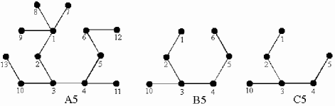
Figure 5: An example of type 1 vertices: for graph A5, $V_{1}(A5)=\{7,8,9,11,12,13\}$, $V_{2}(A5)=\{1,4,6,10\}$, $V_{3}(A5)=\{5\}$ which is type 1, and $V_{4}(A5)=\{2,3\}$.

For $\mathcal{U}_{13}|\psi^{\prime}_{A5}\rangle=|\psi_{A5}\rangle$, the standard construction procedure will result in $\bigotimes\limits_{i=1}^{6}V_{i}\otimes V_{10}|\psi^{\prime}_{B5}\rangle=|\psi_{B5}\rangle$, where $V_{i}\in\mathcal{L}_{1}$ for $i=1,2,3,4,6,10$ and $V_{5}=U_{5}$. Now we again use the construction procedure on qubit $5$ of $B_{3}$ and encode the qubits $5,6$ into a single qubit $5$, as shown in Fig. 5C) ($C5$). This gives $\bigotimes\limits_{i=1}^{4}W_{i}\otimes W_{5}\otimes W_{10}|\psi^{\prime}_{C5}\rangle=|\psi_{C5}\rangle$, where $W_{i}\in\mathcal{L}_{1}$ for $i=1,2,3,4,5,10$. Here $W_{5}$ is induced by $V_{5},V_{6}$ via a similar process as eqs. (12,13,14). Since $V_{6}\in\mathcal{L}_{1}$, we must have $U_{5}=V_{5}\in\mathcal{L}_{1}$, as desired.

In general we can prove $U_{v}\in\mathcal{L}_{1}$ for any type 1 vertex $v\in V_{3}$ as we did for vertex $5$ in the above example of graph $A5$. To be more precise, let $v\in V_{3}(G)$ be a vertex of type 1. For each $v$, carrying out the standard procedure at all $x\in N(v)$ gives us a graph $G_{1}$. We know that each $U_{L}^{(x)}$ must be in $\mathcal{L}_{1}$. Since $v\in V_{2}(\bar{G})$, we then have a non-empty $N(v)\cap V_{1}(\bar{G})$. Again for $G_{1}$ we carry out the standard procedure at $v$, giving us a graph $G_{2}$, and each $U_{L}^{(v)}$ must be in $\mathcal{L}_{1}$. This gives $U_{v}\in\mathcal{L}_{1}$ due to the form of $U_{L}^{(v)}$ in eqs.(27,29).

III.3.2 Type 2

Now we consider the type 2 vertices. We give an example first, to prove that $LU\Leftrightarrow LC$ for graph $A3$ in Fig. 3. $A3$ is a graph without cycles of length 3 and 4, and represents a general graph with four types of vertices. $A3$ is very similar to $A5$, and has the same set of $V_{1},V_{2},V_{3},V_{4}$ as $A5$. The only difference between the two graphs is that in $A3$, vertices $1$ and $6$ are connected to each other. Therefore, following the example for the graph $A5$ shows that for any $\mathcal{U}_{13}|\psi^{\prime}_{A3}\rangle=|\psi_{A3}\rangle$, the standard construction procedure will result in $\bigotimes\limits_{i=1}^{6}V_{i}\otimes V_{10}|\psi^{\prime}_{B3}\rangle=|\psi_{B3}\rangle$, where $V_{i}\in\mathcal{L}_{1}$ for $i=1,2,3,4,6,10$ and $V_{5}=U_{5}$. However, from the structure of $B3$, it is easy to conclude that $V_{5}=U_{5}\in\mathcal{L}_{1}$.

In general, we can prove $U_{v}\in\mathcal{L}_{1}$ for any type 2 vertex $v\in V_{3}$ as we did for vertex $5$ in the above example of graph $A3$. To be more precise, let $v\in V_{3}(G)$ be a vertex of type 2. For each $v$, carrying out the standard procedure at all $x\in N(v)$ gives us a graph $G_{1}$. $G$ contains neither cycles of length $3$ nor $4$, so the same holds for $G_{1}$. Since $v\in V_{4}(\bar{G})$, we have $v\in V_{4}(G_{1})$. Due to Lemma 2, we conclude that $U_{v}\in\mathcal{L}_{1}$.

III.3.3 Type 3

Now we consider the type 3 vertices. Let us first examine an example. Consider the graph $A3^{\prime}$ which is obtained by deleting vertices $2$ and $13$ from graph $A3$. For this new graph with $V(A3^{\prime})=\{1,3,4,5,6,7,8,9,10,11,12\}$, we have $V_{1}(A3^{\prime})=\{7,8,9,10,11,12\}$, $V_{2}(A3^{\prime})=\{1,3,4,6\}$, $V_{3}(A3^{\prime})=\{5\}$ and $V_{4}(A3^{\prime})=\emptyset$. It is easy to see that the vertex $5$ is of type 3. Carrying out the standard procedure at vertices $4$ and $6$ gives a graph $A3^{\prime\prime}$, which is a subgraph of $A3$ with $V(A3^{\prime\prime})=\{1,3,4,5,6,7,8,9,10\}$. Now we see that $5\in V_{4}(A3^{\prime})$, and hence $U_{5}\in\mathcal{L}_{1}$ for any $\bigotimes\limits_{i\in V(A3^{\prime})}U_{i}$ which takes the graph state $|\psi_{A3^{\prime}}\rangle$ to another $11$-qubit stabilizer state.

In general, note that $v\in V_{3}(G)$ is of type 3 only when every vertex $x\in N(v)$ not only connects to some degree one vertices, but also connects to some vertices in $V_{2}(G)$. So the trick is to perform the standard procedure only at all $x\in N(v)$. This gives a graph $G_{2}$. Since $v\in V_{3}(\bar{G})$, we have $v\in V_{4}(G_{2})$. Due to our result in Sec. III A1, we conclude that $U_{v}\in\mathcal{L}_{1}$.

III.4 Some remarks

To summarize, in general we first classify the vertices of $G$ into four types ($V_{1}(G),V_{2}(G),V_{3}(G),V_{4}(G)$). To construct $\mathcal{K}_{n}$, we choose $K_{i}=U_{i}$ for all $i\in V_{3}(G)\cup V_{4}(G)$, and then apply the standard procedure to construct $K_{i}$ for all $i\in V_{1}(G)\cup V_{2}(G)$.

Note that for some graphs for which $V_{3}$ and $V_{4}$ are both empty sets, for instance the graph $B4$ in Fig.4, the general procedure discussed in the above paragraph does not apply directly. This special situation has already been discussed in detail in Sec III B4.

This completes our proof of the Main Theorem.$\square$

III.5 Algorithm for constructing $\mathcal{K}_{n}$

The proof of our Main Theorem implies a constructive procedure for obtaining the local Clifford operation $\mathcal{K}_{n}$ corresponding to a given local unitary operation $\mathcal{U}_{n}$. This procedure is described below. For clarity, the operation “$\times$ is used to denote standard matrix multiplication in $SU(2)$.

[Algorithm: Construction of $\mathcal{K}_{n}$]:

CONSTRUCT-LC[$G$, $\mathcal{U}_{n}$]:

Input: A connected graph $G$ with no cycles of length 3 or 4; a stabilizer state $|\psi_{G}^{\prime}\rangle$ and an LU operation $\mathcal{U}_{n}=\bigotimes_{i=1}^{n}U_{i}$ such that $\mathcal{U}_{n}|\psi_{G}^{\prime}\rangle=|\psi_{G}\rangle$.

Output: An LC operation $\mathcal{K}_{n}=\bigotimes_{i=1}^{n}K_{i}$ such that $\mathcal{K}_{n}|\psi_{G}^{\prime}\rangle=|\psi_{G}\rangle$.

1. Partition $V(G)$ into subsets $V_{1},V_{2},V_{3},V_{4}$.
2. Let $K_{i}\leftarrow U_{i}$ for all $i\in V_{3}\cup V_{4}$.
3. for each $v_{2}\in V_{2}$:
3.1    Calculate $B_{v_{2}}=U_{v_{2}}^{\dagger}Z_{v_{2}}U_{v_{2}}$.
3.2    Find any $F_{v_{2}}\in\mathcal{L}_{1}$ such that $F_{v_{2}}B_{v_{2}}F_{v_{2}}^{\dagger}=Z_{v_{2}}$.
3.3   Calculate $\tilde{U}_{v_{2}}=U_{v_{2}}F_{v_{2}}^{\dagger}$.
3.4    Find $\{w_{1},\dotsc,w_{k}\}\subset V_{1}$ such that $\{w_{j},v_{2}\}\in E(G)$
        for all $1\leq j\leq k$.
3.5    for $j\leftarrow 1$ to $k$
3.5.1      Find any $F_{w_{j}}\in\mathcal{L}_{1}$ such that $F_{w_{j}}B_{w_{j}}F_{w_{j}}^{\dagger}=Z_{w_{j}}$.
3.5.2      Calculate $\tilde{U}_{w_{j}}=H_{w_{j}}U_{w_{j}}F_{w_{j}}^{\dagger}$.
3.5.3    end for
3.6    if $\tilde{U}_{v_{2}}$ is diagonal
3.6.1      Calculate $\tilde{K}_{v_{2}}=\tilde{U}_{v_{2}}\times\tilde{U}_{w_{1}}\dotsc\times\tilde{U}_{w_{k}}$.
3.6.2      Let $\tilde{K}_{w_{j}}=I_{w_{j}}$ for all $j$.
3.6.3      Let $K_{v_{2}}=\tilde{K}_{v_{2}}F_{v_{2}},K_{w_{j}}=H_{w_{j}}\tilde{K}_{w_{j}}F_{w_{j}}$.
3.7    else
3.7.1      Calculate $\tilde{K}_{v_{2}}=\tilde{U}_{v_{2}}X_{v_{2}}\times\tilde{U}_{w_{1}}X_{w_{1}}\dotsc\times\tilde{U}_{w_{k}}X_{w_{k}}$.
3.7.2     Let $\tilde{K}_{w_{j}}=X_{w_{j}}$ for all $j$.
3.7.3     Let $K_{v_{2}}=\tilde{K}_{v_{2}}F_{v_{2}},K_{w_{j}}=H_{w_{j}}\tilde{K}_{w_{j}}F_{w_{j}}$.
3.7.4    end if
3.8 end for
4. return $\mathcal{K}_{n}=\bigotimes_{i=1}^{n}K_{i}$.

III.6 $\delta=2$ graphs beyond the main theorem

In this section, we present a theorem regarding $LU\Leftrightarrow LC$ for $\delta=2$ graphs. We again use $\bar{G}$ to denote the graph obtained by deleting all the degree one vertices from $G$.

[Theorem 2]: $LU\Leftrightarrow LC$ holds for any $\delta=2$ graph $G$ if $\bar{G}$ satisfies the MSC.

[Proof]: The proof is the same as the proof of the Main Theorem in the special case where $V_{3}(G)$ is an empty set. $\square$

Although the proof of Theorem 2 is a special case of the proof of the Main Theorem, Theorem 2 is not a corollary of the Main Theorem. It can be applied to many $\delta=2$ graphs with cycles of length $3$ or $4$, since we know that many $\delta>2$ graphs satisfy the MSC.

IV $\delta>2$ graph states beyond the MSC

From Lemma 3, we know that for graphs of $\delta>2$, our Main Theorem is actually a corollary of Theorem 1. Now an interesting question is: do there exist other graph states with distance $\delta>2$ which are beyond the MSC? The answer is affirmative. Below, in Sec. IVA, we present some examples for the case $n\leq 11$ qubits. In Sec. IVB we construct two series of $\delta>2$ graphs beyond the MSC for $n=2^{m}-1$ ($m\geq 4$) out from error correcting codes with non-Clifford transversal gates. In Sec. IVC, we briefly discuss the $LU\Leftrightarrow LC$ property for $\delta>2$ graphs.

IV.1 $\delta>2$ graphs beyond the MSC for minimal $n$

Generally the distance of a graph state can be upper bounded by $2\left\lfloor\frac{n}{6}\right\rfloor+1$ for a graph whose elements in $\mathcal{S}$ have even weight, which only happens when $n$ is even. For the other graphs, the distance is upper bounded by $2\left\lfloor\frac{n}{6}\right\rfloor+1$, if $n\equiv 0$ mod 6, $2\left\lfloor\frac{n}{6}\right\rfloor+3$, if $n\equiv 5$ mod 6, and $2\left\lfloor\frac{n}{6}\right\rfloor+2$, otherwiseRains2 .

Our numerical calculations show that there are no $\delta>2$ graphs beyond the MSC for $n<9$. Among all the $440$ LC non-equivalent connected graphs of $n=9$, there are only three $\delta>2$ graphs beyond the MSC. All of them are of distance three, which are shown as graphs A6, B6, and C6 in Fig. 6. Among all the $3132$ LC non-equivalent connected graphs of $n=10$, there are only nine $\delta>2$ graphs beyond the MSC. Eight of them are of distance three, only one is of distance four. The distance four graph of $n=10$ beyond the MSC is shown as graph D6 in Fig. 6. Among all the $40457$ LC non-equivalent connected graphs of $n=11$, there are only $46$ $\delta>2$ graphs beyond the MSC. $37$ of them are of distance three and $9$ are of distance four.

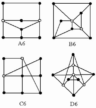
Figure 6: A6, B6, C6: Three $\delta=3$ graphs beyond the MSC for $n=9$; D6: The only one $\delta=4$ graph beyond the MSC for $n=10$. In each graph all the black vertices are minimal elements which are just generators of the corresponding $\mathcal{M}$, and all the white vertices are not in $\mathcal{M}$.

IV.2 Graphs derived from codes with non-Clifford transversal gates

In this section we construct other two series of $\delta>2$ graphs beyond the MSC for $n=2^{m}-1$ ($m\geq 4$) from error correcting codes with non-Clifford transversal gates.

It is well-known that transversal gates on quantum codes, i.e. logical unitary operations which could be realized via a bitwise manner, is crucial for fault-tolerant quantum computingNielsen ; Gottesman . General single qubit transversal gates on an $n$-qubit code $Q$ is of the form $\mathcal{U}_{n}$. However, only Clifford transversal gates $\mathcal{K}_{n}$ are relatively easy to find from symmetries of the stabilizerNielsen ; Gottesman , while it is hard to find non-Clifford transversal gates for a given stabilizer code.

To construct the CSS code with transversal gates

$$\exp\left(-i\frac{\pi}{2^{m-1}}\,{Z_{L}}\right)\cong\bigotimes_{i=1}^{2^{m}-1}\exp\left(i\frac{\pi}{2^{m-1}}\,Z_{i}\right),$$ (40)

consider the first order punctured Reed-Muller code $C_{1}=RM^{*}(1,m)$ with parameters $[2^{m}-1,m+1,2^{m-1}-1]$ and its even subcode $C_{2}=even(RM^{*}(1,m))$ with parameters $[2^{m}-1,m,2^{m-1}]$MacWilliams . It is well-known that the dual code of $C_{1}$ is the binary Hamming code with parameters $[2^{m}-1,2^{m}-1-m,3]$. Then this gives a series of quantum codes with parameters $[2^{m}-1,1,3]$. For a given $m$, the code is spanned by $|\bar{0}\rangle=\sum_{c\in C_{2}}|c\rangle$ and $|\bar{1}\rangle=\sum_{c\in C_{1}-C_{2}}|c\rangle$. The computational basis vectors on which $|\bar{0}\rangle$ has support have weight $0$ or $2^{m-1}$ and those of $|\bar{1}\rangle$ have weight $2^{m-1}-1$ or $2^{m}-1$Feng . Therefore, $\exp{\left(-i\frac{\pi}{2^{m-1}}{Z_{L}}\right)}$ is a valid transversal gate.

Similar to the classical Reed-Muller codes, from the point of view of code parameters, these quantum codes become weaker as their length increases. However, non-Clifford operations are not all equal; some are more complex than others, even for fixed qubit number. Note that $\exp\left(-i\frac{\pi}{2^{m-1}}\,{Z_{L}}\right)\in\mathcal{C}_{k}$ with $k=m-1$, where $\mathcal{C}_{k}$ is defined by

$$\mathcal{C}_{k+1}=\{U\in U(\mathcal{H})|U\mathcal{C}_{1}U^{\dagger}\subseteq\mathcal{C}_{k}\},$$ (41)

where $\mathcal{C}_{1}$ is the Pauli group, and generally gates in $\mathcal{C}_{k}$ with larger $k$ are strongerGot . Hence it worths constructing codes with transversal $\mathcal{C}_{k}$ gates for any $k$.

Note that the graphs corresponding to $|0_{L}\rangle$s of the code always have distance $3$ for any $m$, and the graphs corresponding to $|+_{L}\rangle$s of the code always have distance $4$ for any $m$. It is straightforward to show that for any $m$, only $Z$ appears on all the qubits in $\mathcal{M}$ for both $|0_{L}\rangle$ and $|+_{L}\rangle$. This then gives two series of $\delta>2$ graphs beyond the MSC. The graphs for $m=4,5$ are shown in Fig. 7 and 8.

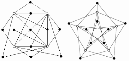
Figure 7: $d\geq 3$ graphs beyond the MSC. The left graph corresponds to the $|0_{L}\rangle$ state of the 15 qubit code with transversal $T$ gate. And the right one is a graph corresponds to $|+_{L}\rangle$, getting from Rau . In each graph all the black vertices are minimal elements which are just generators of the corresponding $\mathcal{M}$, and all the white vertices are not in $\mathcal{M}$.

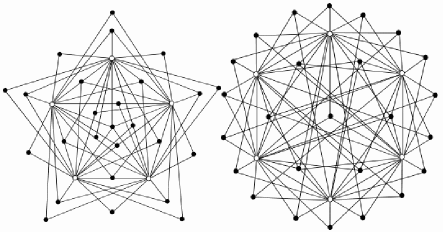
Figure 8: $d\geq 3$ graphs beyond the MSC. The left graph corresponds to the $|0_{L}\rangle$ state of the 31 qubit code with transversal $\exp{\left(-i\frac{\pi}{16}Z_{L}\right)}$ gate. And the right one is a graph corresponds to $|+_{L}\rangle$. In each graph all the black vertices are minimal elements which are just generators of the corresponding $\mathcal{M}$, and all the white vertices are not in $\mathcal{M}$.

IV.3 $LU\Leftrightarrow LC$ property for $\delta>2$ graphs

It is natural to ask whether we could use the same strategy to prove $LU\Leftrightarrow LC$ for those $\delta>2$ graph states beyond the MSC as we did for $\delta=2$ graphs.

First of all, it is noted that a similar deletion of a degree $d-1$ vertex is possible. Take the above $\delta=3$ graph in Fig. 6 A6 for instance. Denote the two white vertices by $2,3$, and the degree two vertex which connects to $2,3$ by $1$. Then the stabilizer of $1,2,3$, up to LC, can be written as

$$Z_{1}Z_{2}Z_{3},X_{1}X_{2}R_{j},X_{1}X_{2}R_{k}$$ (42)

where $R_{j},R_{k}$ denotes the operators on the other qubits apart from $1,2,3$.

Now recall the $n$-qubit quantum code ${Q}_{e}^{(n)}$ with stabilizer $\mathcal{S}({Q_{e}^{(n)}})=\{I^{\otimes{n}},Z^{\otimes{n}}\}$ is a quantum version of the $[n,n-1,2]$ classical binary zero-sum code (or even weight code). The basis of ${Q}_{e}^{(n)}$ can be simply chosen as all the codewords with even weight, and any of the $n$ qubits can be regarded as a parity qubit of the other $n-1$ qubits. In this sense, $Q_{e}^{(n)}$ encoding $n$ qubits into $n-1$ qubit, we will always choose the basis for $n-1$ logical qubits to be that of omitting the first qubit. For instance, if $n=3$ (as mentioned in graph A6 of Fig. 6, the stabilized subspace of $Z_{1}Z_{2}Z_{3}$ is spanned by

$$\{|0_{1}0_{2}0_{3}\rangle,|1_{1}0_{2}1_{3}\rangle,|1_{1}1_{2}0_{3}\rangle,|0_{1}1_{2}1_{3}\rangle\},$$ (43)

which could be viewed as two logical qubits:

$$\{|00\rangle_{L}=|0_{1}0_{2}0_{3}\rangle,|01\rangle_{L}=|1_{1}0_{2}1_{3}\rangle,$$

$$|10\rangle_{L}=|1_{1}1_{2}0_{3}\rangle,|11\rangle_{L}=|0_{1}1_{2}1_{3}\rangle\},$$ (44)

where the first physical qubit acts as a parity qubit of the other two.

Any LU operation $\mathcal{F}_{n}=\bigotimes_{i=1}^{n}F_{i}$ where each $F_{i}$ is diagonal preserves $Q_{e}$ and will induce an diagonal logical operation $F_{L}$ on the $n-1$ logical qubits.

[Proposition 2]: For an $n$-qubit even weight code $Q_{e}$, if $F_{L}\in\mathcal{L}_{n-1}$, then $F_{i}\in\mathcal{L}_{1}$ for all $i=1,\ldots,n$.

[Proof]: Since $F_{L}$ is diagonal, it preserves $Z_{i}$ for all $i=2,\ldots,n$. Let $F_{i}=diag\{1,e^{i\theta_{i}}\}$, direct calculation shows $F_{L}X_{2}F_{L}^{\dagger}\in\mathcal{G}_{n-1}$ if and only if both $e^{2i\theta_{1}}=\pm 1$ and $e^{2i\theta_{2}}=\pm 1$, i.e. $F_{1},F_{2}\in\mathcal{L}_{1}$. Similar procedure works for $i=3,\ldots,n$.$\square$

However, generally $F_{L}$ is a non-local operation on the $n-1$ logical qubits, contrary to the $\delta=2$ case, where the local operation can only induce a local operation on the single logical qubit. Therefore, it is non-trivial to delete a degree $d-1$ vertex.

A possible way to fix this problem may be to further investigate the effect of some non-local gates (in this example, two-qubit gates) which relate the two graph states. Then we could use Proposition 2 to prove $LU\Leftrightarrow LC$ for the original graph before deletion of the vertex. This idea does work in the case of the particular structure of the graph A6 in Fig. 6, after a subtle analysis on the structure of $\mathcal{S}$.

Our Proposition 2 takes the first step to investigate the $LU\Leftrightarrow LC$ property for $\delta>2$ graphs beyond the MSC, which is also based on the subgraph structure. However, it is not our hope that the idea of induction will final lead to a solution to the most general case. For instance, it is noted that $|{\psi}\rangle$ satisfying the MSC does not necessarily mean $\mathcal{S}(|{\psi}\rangle)=\mathcal{M}(|{\psi}\rangle)$ , although exceptions are likely rare. We have found only two LU inequivalent examples for $n\leq 9$, which are shown below in Fig. 9.

Figure 9: Two $n=8$ graphs satisfying the MSC, but $\mathcal{S}(|{\psi}\rangle)\neq\mathcal{M}(|{\psi}\rangle)$.

Note both of the two graphs in Fig. 9 are of $n=8$. There exist two graphs satisfying the MSC but $\mathcal{S}\neq\mathcal{M}$ for $n=8$, however there does not exist any graph of this property for $n=9$. This interesting phenomenon implies that the structure of $\mathcal{M}$ is a global rather than a local property of graph states, which cannot be simply characterized by the idea of induction.

V Conclusion and discussion

In this paper, we broaden the understanding of what graph and stabilizer states are equivalent under local Clifford operations. We prove that $LU\Leftrightarrow LC$ equivalence holds for all graph states for which the corresponding graph contains neither cycles of length $3$ nor $4$. We also show that $LU\Leftrightarrow LC$ equivalence holds for distance $\delta=2$ graph states if their corresponding graph satisfies the MSC after deleting all the degree one vertices. The relation between our results and those of Van den Nest et al.’s is summarized in Fig. 1. It is clearly seen from the figure that graphs in area $D$ have no intersection with those in $C$, i.e. graph states of distance $\delta=2$ are beyond Van den Nest et al.’s MSC. The intersection of graphs in area $B$ and $C$ are graphs without degree one vertices as well as cycles of length $3$ and $4$.

We find a total of $58$ $\delta>2$ graphs beyond the MSC up to $n=11$, via numerical search; among these, only $10$ are of $\delta=4$ while the other $48$ have distance $\delta=3$. This implies that $\delta>2$ graphs beyond the MSC are rare among all the graph states, and are not easy to find and characterize. However, we also explicitly construct two series of $\delta>2$ graphs using quantum error correcting codes which have non-Clifford transversal gates. We expect that the existence of other such quantum codes will provide insight in seeking additional $\delta>2$ graphs beyond the MSC. All graph states discussed in this paragraph belong in area $E$ in Fig. 1. For most of the graphs in area $E$, the $LU\Leftrightarrow LC$ equivalence question remains open. We discussed some possibilities for resolving this equivalence question in Sec. IV, using even weight codes rather than the simple repetition codes.

Our main new technical tool for understanding $LU\Leftrightarrow LC$ equivalence is the idea, introduced in Sec. III, of encoding and decoding of repetition codes. We hope that this tool, and our other results, will help shed light on the unusual equivalences of multipartite entangled states represented by stabilizers and graphs, and the intricate relationship between entanglement and quantum error correction codes which allow non-Clifford transversal gates.

References

- (1) M. A. Nielsen and I. L. Chuang, Quantum Computation and Quantum Information, (Cambridge University Press, Cambridge, UK, 2000).
- (2) D. Gottesman. Stabilizer codes and quantum error correction. PhD thesis, Caltech, 1997. quant-ph/9705052.
- (3) R. Raussendorf, D.E. Browne, and H. J. Briegel, Phys. Rev. A68, 022312 (2003).
- (4) W. Dur, H. Aschauer, and H. J. Briegel, Phys. Rev. Letts. 91, 107903 (2003).
- (5) M. Hein, J. Eisert, and H. J. Briegel, Phys. Rev. A69, 062311 (2004).
- (6) M. Hein, W. Dur, J. Eisert, R. Raussendorf, M. Van den Nest, and H. J. Briegel, E-print quant-ph/0602096.
- (7) D. Schlingemann, and R.F. Werner, Phys. Rev. A65, 012308 (2002).
- (8) D. W. Vidal, and J. I. Cirac, Phys. Rev. A62, 062314 (2000).
- (9) A. Acn, A. Andrianov, and L. Costa et al., Phys. Rev. Letts. 85, 1560 (2000).
- (10) F. Verstraete, J. Dehaene, B. De Moor, and H. Verschelde, Phys. Rev. A65, 052112 (2002).
- (11) M. Van den Nest, J. Dehaene, and B. De Moor, Phys. Rev. A69, 022316 (2004)
- (12) L. E. Danilesen and M. G. ParKer, E-print math.CO/0504522; L. E. Danilesen, On Self-Dual QuantumCodes, Graphs, and Boolean Functions, Master thesis, University of Bergen, Norway (2005), E-print quant-ph/0503236.
- (13) M. Van den Nest, and B. De Moor, E-print math.CO/0510246.
- (14) M. Van den Nest, J. Dehaene, B. De Moor, Phys. Rev. A71, 062323 (2005).
- (15) E. M. Rains, E-print quant-ph/9704043.
- (16) D. M. Greenberger, M. Horne, A. Zeilinger, in Bell’s theorem, Quantum Theory, and Conceptions of the Universe, ed. M. Kafatos, Kluwer Academic Publishers (1989).
- (17) E. M. Rains, and N. J. A. Sloane, E-print math.CO/0208001.
- (18) F. J. MacWilliams, N. J. A. Sloane, The Theory of Error-Correcting Codes, North-Holland Publishing Company, Amsterdam (1977).
- (19) K. Q. Feng, Algebraic Theory of Error-Correcting Codes, (Tsinghua University Press, 2005).
- (20) D. Gottesman, and Isaac Chuang, Nature 402, 390 (1999).
- (21) R. Raussendorf, J. Harrington, and K. Goyal, E-print quant-ph/0510135.