Non-Markovian generalization of the Lindblad theory of open quantum systems

Abstract

A systematic approach to the non-Markovian quantum dynamics of open systems is given by the projection operator techniques of nonequilibrium statistical mechanics. Combining these methods with concepts from quantum information theory and from the theory of positive maps, we derive a class of correlated projection superoperators that take into account in an efficient way statistical correlations between the open system and its environment. The result is used to develop a generalization of the Lindblad theory to the regime of highly non-Markovian quantum processes in structured environments.

I Introduction

The theoretical description of relaxation and decoherence processes in open quantum systems often leads to a non-Markovian dynamics which is determined by pronounced memory effects TheWork . Strong system-environment couplings REIBOLD ; HU , correlations and entanglement in the initial state INGOLD ; BUZEK , interactions with environments at low temperatures and with spin baths LOSS , finite reservoirs GEMMER2005 ; GMM , and transport processes in nano-structures FOURIER can lead to long memory times and to a failure of the Markovian approximation.

A systematic approach to non-Markovian dynamics is provided by the projection operator techniques NAKAJIMA ; ZWANZIG ; HAAKE which are extensively used in nonequilibrium thermodynamics and statistical mechanics KUBO . These techniques are based on the introduction of a certain projection superoperator ${\mathcal{P}}$ which acts on the states of the total system. The superoperator ${\mathcal{P}}$ is the mathematical expression for the idea of the elimination of degrees of freedom from the complete description of the states of the total system: If $\rho$ is the full density matrix of the composite system, the projection ${\mathcal{P}}\rho$ represents a certain approximation of $\rho$ which leads to a simplified effective description of the dynamics through a reduced set of variables. The projection ${\mathcal{P}}\rho$ is therefore referred to as the relevant part of the density matrix.

With the help of the projection operator techniques one derives closed dynamic equations for the relevant part of the density matrix. The equation of motion for ${\mathcal{P}}\rho$ can either be the Nakajima-Zwanzig equation NAKAJIMA ; ZWANZIG , an integrodifferential equation with a retarded memory kernel, or else the time-convolutionless master equation, which is a time-local differential equation of first order involving a time-dependent generator SHIBATA . In most cases these equations are used as starting point for the derivation of effective master equations through a systematic perturbation expansion with respect to the strength of the system-environment coupling.

In the standard approach to the dynamics of open systems one chooses a projection superoperator which is defined by the expression ${\mathcal{P}}\rho=\rho_{S}\otimes\rho_{0}$, where $\rho_{S}={\mathrm{tr}}_{E}\rho$ represents the reduced density matrix of the open system, ${\mathrm{tr}}_{E}$ denoting the trace over the environmental Hilbert space, and $\rho_{0}$ is some fixed environmental state. A superoperator of this form projects the total state $\rho$ onto a tensor product state, i. e., onto a state without any statistical correlations between system and environment. We emphasize that this ansatz does not imply (as is sometimes claimed) that one completely ignores all system-environment correlations. It only presupposes that all correlations which are present in the initial state or are generated during the time-evolution can be treated as perturbations within the framework of the projection operator techniques.

The projection onto a tensor product state is widely used in studies of open quantum systems. It is often applicable in the case of weak system-environment couplings. Usually, the perturbation expansion is restricted to the second order (known as Born approximation), from which one derives, with the help of certain further assumptions, a Markovian quantum master equations in Lindblad form GORINI ; LINDBLAD ; SPOHN . In this paper the quantum dynamics of an open system is said to be non-Markovian if the time-evolution of its reduced density matrix cannot be described (to the desired degree of accuracy) by means of a closed master equation with a time-independent generator in Lindblad form.

A possible approach to large deviations from Markovian behavior consists in carrying out the perturbation expansion to higher orders in the system-environment coupling (several examples are discussed in Ref. TheWork ). However, this approach is often limited by the increasing complexity of the resulting equations of motion. Moreover, the perturbation expansion may not converge uniformly in time, such that higher orders only improve the quality of the approximation of the short-time behavior, but completely fail in the long-time limit BBP .

There is however a further promising strategy: To treat highly non-Markovian processes in a more efficient way one can replace the tensor product state used in the standard Born approximation by a certain correlated system-environment state. This approach has been proposed by Esposito and Gaspard GASPARD1 ; GASPARD2 and by Budini BUDINI05 to derive effective master equations within second order perturbation theory that describe strong non-Markovian effects. It has been demonstrated in Ref. BGM that this idea can be formulated in terms of a positive projection superoperator ${\mathcal{P}}$ which projects any state onto a correlated system-environment state, i. e., onto a state that contains statistical correlations between certain system and environment states. This formulation allows an immediate application of the projection operator techniques to correlated system-environment states, and to carry out the perturbation expansion to higher orders in a systematic way. An example is discussed in Ref. BGM , where the master equations of second and of fourth order corresponding to a correlated projection superoperator have been constructed.

The application of a correlated projection superoperator implies that the relevant part ${\mathcal{P}}\rho$ can no longer be expressed in terms of the reduced density matrix alone. Hence, employing a correlated projection superoperator one enlarges the set of relevant variables to capture those statistical correlations that are responsible for strong non-Markovian effects.

In the present paper we discuss this idea of using correlated projection superoperators in the analysis of non-Markovian dynamics. On the basis of certain general physical conditions we derive in Sec. II a representation theorem for a class of correlated projection superoperators that are appropriate for the application of the projection operator techniques.

A central problem of the theory of non-Markovian processes is the formulation of appropriate master equations that preserve the normalization and the positivity of the density matrix (see, e. g., the discussion in Refs. BARNETT ; BUDINI04 ; LIDAR ; MANISCALCO ). In Sec. III we develop the general structure of such master equations which results form the application of a correlated projection superoperator. Given a superoperator that projects onto a separable quantum state one can construct an embedding of the underlying dynamics into a Lindblad dynamics on a suitably extended state space. Employing this embedding we derive a general class of physically acceptable master equations which represents a generalization of the Lindblad theory to the regime of highly non-Markovian quantum dynamics. Section IV contains some conclusions.

II Correlated projection superoperators

II.1 General conditions

The Hilbert spaces of the open system $S$ and of its environment $E$ are denoted by ${\mathcal{H}}_{S}$ and ${\mathcal{H}}_{E}$, respectively. The state space of the composite system is given by the tensor product ${\mathcal{H}}={\mathcal{H}}_{S}\otimes{\mathcal{H}}_{E}$. States of the composite system are represented by density matrices $\rho$ on ${\mathcal{H}}$ satisfying $\rho\geq 0$ and ${\mathrm{tr}}\rho=1$, where ${\mathrm{tr}}$ is the trace taken over the total state space. The reduced density matrix $\rho_{S}$ of subsystem $S$ is given by the partial trace taken over the Hilbert space ${\mathcal{H}}_{E}$, i. e. $\rho_{S}={\mathrm{tr}}_{E}\rho$. Correspondingly, the partial trace over ${\mathcal{H}}_{S}$ will be denoted by ${\mathrm{tr}}_{S}$.

A superoperator ${\mathcal{P}}$ is a linear map ${\mathcal{O}}\mapsto{\mathcal{P}}{\mathcal{O}}$ which takes any operator ${\mathcal{O}}$ on the total state space ${\mathcal{H}}$ to an operator ${\mathcal{P}}{\mathcal{O}}$ on ${\mathcal{H}}$. We consider here superoperators with the following properties.

1. The map ${\mathcal{P}}$ is a projection superoperator:

$${\mathcal{P}}^{2}={\mathcal{P}}.$$ (1)

It is this formal property that allows the application of the projection operator techniques. For an efficient performance of these techniques the projection ${\mathcal{P}}\rho$ should represent a suitable approximation of $\rho$. A natural minimal requirement is therefore that for any physical state $\rho$ the projection ${\mathcal{P}}\rho$ is again a physical state, i. e., a positive operator with unit trace. This means that ${\mathcal{P}}$ is a positive and trace preserving map, namely $\rho\geq 0$ implies ${\mathcal{P}}\rho\geq 0$, and ${\mathrm{tr}}\{{\mathcal{P}}\rho\}={\mathrm{tr}}\rho$.

2. We consider projection superoperators of the following general form:

$${\mathcal{P}}=I_{S}\otimes\Lambda,$$ (2)

where $I_{S}$ denotes the unit map acting on operators on ${\mathcal{H}}_{S}$, and $\Lambda$ is a linear map that takes operators on ${\mathcal{H}}_{E}$ to operators on ${\mathcal{H}}_{E}$. A projection superoperator of this form leaves the system $S$ unchanged and acts nontrivially only on the variables of the environment $E$. As a consequence of the positivity of ${\mathcal{P}}$ and of condition (2) the map $\Lambda$ must be $N_{S}$-positive, where $N_{S}$ is the dimension of ${\mathcal{H}}_{S}$ (see, e. g., Ref. KOSSAKOWSKI ). In the following we use the stronger condition that $\Lambda$ is completely positive, because completely positive maps allow for a simple mathematical characterization (see Sec. II.2).

We discuss the implications of these conditions. From Eqs. (1) and (2) we get that $\Lambda$ itself must be a projection, namely $\Lambda^{2}=\Lambda$. Moreover, since ${\mathcal{P}}$ is trace-preserving, the map $\Lambda$ must also be trace-preserving. Hence, we find that $\Lambda$ represents a completely positive and trace-preserving map (CPT map, or quantum channel) which operates on the variables of the environment and has the property of a projection. A further physically reasonable consequence of the positivity of $\Lambda$ and of Eq. (2) is that ${\mathcal{P}}$ maps separable (classically correlated) states to separable states, which means that the projection does not create entanglement between system and environment.

An important goal is, of course, the determination of the reduced density matrix $\rho_{S}$ of the open quantum system. Using Eq. (2) and that $\Lambda$ is trace-preserving we get the relation

$$\rho_{S}\equiv{\mathrm{tr}}_{E}\rho={\mathrm{tr}}_{E}\{{\mathcal{P}}\rho\}.$$ (3)

This relation connects the density matrix of the reduced system with the projection of a given state $\rho$ of the total system. It states that, in order to determine $\rho_{S}$, we do not really need the full density matrix $\rho$, but only its projection ${\mathcal{P}}\rho$. Thus, ${\mathcal{P}}\rho$ contains the full information needed to reconstruct the reduced system’s state.

II.2 Representation theorem

We derive a representation theorem for the projection superoperator ${\mathcal{P}}$ from the basic conditions formulated in Sec. II.1 [see Eq. (12) below]. Since $\Lambda$ is supposed to be a CPT map one could use, of course, the Kraus-Stinespring representation KRAUS ; STINESPRING for completely positive maps. However, for our purposes another representation is much more appropriate, which will be derived now.

We will use the following fact from linear algebra. Consider a linear operator $L:V\mapsto V$ which acts on some Hilbert space $V$ and has the property $L^{2}=L$. Then there exist linear independent vectors $|f_{i}\rangle$ and linear independent vectors $|e_{i}\rangle$ such that $\langle f_{i}|e_{j}\rangle=\delta_{ij}$ and

$$L|v\rangle=\sum_{i}|f_{i}\rangle\langle e_{i}|v\rangle$$ (4)

for all $|v\rangle\in V$. Conversely, given two linear independent sets $\{|f_{i}\rangle\}$ and $\{|e_{i}\rangle\}$ of vectors in $V$ with $\langle f_{i}|e_{j}\rangle=\delta_{ij}$, then Eq. (4) defines a linear operator with the property $L^{2}=L$. Note that we neither require that the $|f_{i}\rangle$ or the $|e_{i}\rangle$ are orthogonal, nor that $L$ is Hermitian.

Let us apply this fact to linear maps on the Hilbert-Schmidt space, i. e., we take $V$ to be the vector space of operators on ${\mathcal{H}}_{E}$ with the scalar product:

$$(X,Y)\equiv{\mathrm{tr}}_{E}\{X^{\dagger}Y\}.$$

Then we find that any linear map $\Lambda$ can be represented in the form

$$\Lambda X=\sum_{i}B_{i}(A_{i},X)=\sum_{i}{\mathrm{tr}}_{E}\{A^{\dagger}_{i}X\}B_{i}$$

with two sets $\{A_{i}\}$ and $\{B_{i}\}$ of linear independent operators on ${\mathcal{H}}_{E}$, and that the condition $\Lambda^{2}=\Lambda$ is satisfied if and only if $(B_{i},A_{j})=\delta_{ij}$. Since $\Lambda$ preserves the Hermiticity of operators, the operators $A_{i}$ and $B_{i}$ can be chosen to be Hermitian. Hence, we obtain the representation:

$$\Lambda X=\sum_{i}{\mathrm{tr}}_{E}\{A_{i}X\}B_{i},$$ (5)

where $\{A_{i}\}$ and $\{B_{i}\}$ are two sets of linear independent Hermitian operators satisfying:

$${\mathrm{tr}}_{E}\{B_{i}A_{j}\}=\delta_{ij}.$$ (6)

The condition that $\Lambda$ is trace-preserving takes the form:

$$\sum_{i}({\mathrm{tr}}_{E}B_{i})A_{i}=I_{E}.$$ (7)

Finally, we have to formulate the condition of the complete positivity of the map $\Lambda$. A given map $\Lambda$ is completely positive if and only if

$$(I_{E}\otimes\Lambda)(|\psi\rangle\langle\psi|)\geq 0,$$ (8)

where

$$|\psi\rangle=\sum_{\alpha}|\alpha\rangle\otimes|\alpha\rangle$$

is a maximally entangled vector in ${\mathcal{H}}_{E}\otimes{\mathcal{H}}_{E}$, and $\{|\alpha\rangle\}$ is an orthonormal basis for ${\mathcal{H}}_{E}$. To evaluate condition (8) we first note that

$$(I_{E}\otimes\Lambda)(|\psi\rangle\langle\psi|)=\sum_{\alpha\beta}|\alpha\rangle\langle\beta|\otimes\Lambda(|\alpha\rangle\langle\beta|).$$ (9)

On using the representation (5) one finds

$$\Lambda(|\alpha\rangle\langle\beta|)=\sum_{i}\langle\beta|A_{i}|\alpha\rangle B_{i}=\sum_{i}\langle\alpha|A_{i}^{T}|\beta\rangle B_{i},$$ (10)

where $A_{i}^{T}$ denotes the transpose of the operator $A_{i}$ with respect to the given basis $\{|\alpha\rangle\}$. Inserting Eq. (10) into Eq. (9) we obtain

$$(I_{E}\otimes\Lambda)(|\psi\rangle\langle\psi|) = \sum_{i}\sum_{\alpha\beta}|\alpha\rangle\langle\alpha|A_{i}^{T}|\beta\rangle\langle\beta|\otimes B_{i}$$

$$= \sum_{i}A_{i}^{T}\otimes B_{i}.$$

We conclude that a necessary and sufficient condition for $\Lambda$ to be completely positive is given by the inequality

$$\sum_{i}A_{i}^{T}\otimes B_{i}\geq 0.$$ (11)

Employing Eqs. (5) and (2) we obtain the following representation for the projection superoperator ${\mathcal{P}}$,

$${\mathcal{P}}\rho=\sum_{i}{\mathrm{tr}}_{E}\{A_{i}\rho\}\otimes B_{i}.$$ (12)

Given observables $A_{i}$ and $B_{i}$ that satisfy Eqs. (6), (7), and (11), this equation defines a projection superoperator which fulfills the general conditions formulated in Sec. II.1. Conversely, given a projection which fulfills the conditions of Sec. II.1, there exist observables $A_{i}$ and $B_{i}$ satisfying Eqs. (6), (7), and (11) such that Eq. (12) holds. There are in general many different sets of operators $A_{i}$, $B_{i}$ that represent a given ${\mathcal{P}}$. If we have a particular set of such operators, then the operators

$$A^{\prime}_{i}=\sum_{j}u_{ij}A_{j},\qquad B^{\prime}_{i}=\sum_{j}v_{ij}B_{j},$$

represent the same projection, where $u=(u_{ij})$ and $v=(v_{ij})$ are real, non-singular matrices related by $u^{T}v=I$.

II.3 Examples

Within the standard approaches one considers a projection superoperator of the form

$${\mathcal{P}}\rho=({\mathrm{tr}}_{E}\rho)\otimes\rho_{0},$$ (13)

where $\rho_{0}$ is any fixed environmental density matrix. Using a projection of this form one assumes that the states of the total system may be approximated by certain tensor products, describing states without statistical dependencies between system and environment. The projection (13) naturally fits into the general scheme developed above if we take a single $A=I_{E}$ and a single $B=\rho_{0}$. The conditions (6), (7), and (11) are then satisfied and Eq. (12) obviously reduces to Eq. (13)

In the general case, a projection ${\mathcal{P}}\rho$ of the form of Eq. (12) does not represent a simple product state. We therefore call such ${\mathcal{P}}$ correlated projection superoperators. They project onto states that contain statistical correlations between the system $S$ and its environment $E$. In the following we will consider the case that one can find a representation of the projection with positive operators $A_{i}\geq 0$ and $B_{i}\geq 0$. Equation (11) is then trivially satisfied. Without restriction we may assume that the $B_{i}$ are normalized to unit trace, such that condition (7) reduces to the simple form $\sum_{i}A_{i}=I_{E}$. Under these conditions ${\mathcal{P}}$ projects any state $\rho$ onto a state which can be written as a sum of tensor products of positive operators. In the theory of entanglement (see, e. g., Ref. ALBER ) such states are called separable or classically correlated WERNER . Using a projection superoperator of this form, one thus tries to approximate the total system’s states by a classically correlated state. The general representation of Eq. (12) includes the case of projection superoperators that project onto inseparable, entangled quantum states. We will not pursue here this possibility further, and restrict ourselves to positive $A_{i}$ and $B_{i}$ in the following.

A straightforward example for a separable projection superoperator is obtained through the following construction GASPARD1 ; BUDINI05 ; BGM . We take any orthogonal decomposition of the unit operator $I_{E}$ on the state space of the environment, i. e., a collection of ordinary projection operators $\Pi_{i}$ on ${\mathcal{H}}_{E}$ which satisfy

$$\Pi_{i}\Pi_{j}=\delta_{ij}\Pi_{j},\qquad\sum_{i}\Pi_{i}=I_{E}.$$

Then we choose:

$$A_{i}=\Pi_{i},\qquad B_{i}=\frac{\Pi_{i}\rho_{0}\Pi_{i}}{{\mathrm{tr}}_{E}\{\Pi_{i}\rho_{0}\}}.$$

It is easy to verify that with this choice the conditions (6), (7), and (11) are satisfied. The explicit form of the projection superoperator is given by

$${\mathcal{P}}\rho=\sum_{i}{\mathrm{tr}}_{E}\left\{\Pi_{i}\rho\right\}\otimes\frac{\Pi_{i}\rho_{0}\Pi_{i}}{{\mathrm{tr}}_{E}\{\Pi_{i}\rho_{0}\}}.$$ (14)

II.4 Relevant states and observables

Given a projection superoperator we define the relevant states as the states in the range of ${\mathcal{P}}$, i. e., for which the relation

$${\mathcal{P}}\rho_{\mathrm{rel}}=\rho_{\mathrm{rel}}$$

holds. We see that these states are of the form

$$\rho_{\mathrm{rel}}=\sum_{i}\rho_{i}\otimes B_{i},$$

where the $\rho_{i}$ may be any positive matrices such that $\sum_{i}{\mathrm{tr}}_{S}\rho_{i}=1$. Hence, the manifold of the relevant states is determined by the operators $B_{i}$.

One can transfer this concept from states (Schrödinger picture) to observables (Heisenberg picture). A Hermitian operator ${\mathcal{O}}_{{\mathrm{rel}}}$ on the total state space is said to be a relevant observable if the relation

$${\mathrm{tr}}\{{\mathcal{O}}_{{\mathrm{rel}}}({\mathcal{P}}\rho)\}={\mathrm{tr}}\{{\mathcal{O}}_{{\mathrm{rel}}}\rho\}$$

holds true for all states $\rho$. This means that the expectation value of a relevant observable in any state of the composite system is left unchanged under the application of the projection superoperator ${\mathcal{P}}$.

Introducing the adjoint map ${\mathcal{P}}^{\dagger}$ (defined with respect to the Hilbert-Schmidt scalar product for operators on the total state space) we can reformulate this condition as

$${\mathcal{P}}^{\dagger}{\mathcal{O}}_{{\mathrm{rel}}}={\mathcal{O}}_{{\mathrm{rel}}}.$$

Hence, the relevant observables are those observables which are invariant under the application of the adjoint projection. From the representation (12) we get:

$${\mathcal{P}}^{\dagger}{\mathcal{O}}=\sum_{i}{\mathrm{tr}}_{E}\{B_{i}{\mathcal{O}}\}\otimes A_{i},$$ (15)

from which we infer that the relevant observables must be of the form

$${\mathcal{O}}_{{\mathrm{rel}}}=\sum_{i}{\mathcal{O}}^{i}_{S}\otimes A_{i},$$ (16)

where the ${\mathcal{O}}^{i}_{S}$ are arbitrary observables of the subsystem $S$. The structure of the relevant observables is thus determined by the operators $A_{i}$.

III Dynamics

III.1 General formulation

The dynamics of the total system is given by

$$\rho(t)=U(t)\rho(0)U^{\dagger}(t),$$ (17)

where $U(t)$ denotes the unitary time-evolution operator. Given a projection superoperator of the form of Eq. (12) one introduces the dynamical variables:

$$\rho_{i}(t)={\mathrm{tr}}_{E}\left\{A_{i}\rho(t)\right\}.$$ (18)

Since the $A_{i}$ are positive operators, we have $\rho_{i}(t)\geq 0$, and by use of Eq. (3) and of the normalization ${\mathrm{tr}}_{E}B_{i}=1$ we find that the reduced density matrix is obtained from

$$\rho_{S}(t)=\sum_{i}\rho_{i}(t).$$

The normalization condition reads:

$${\mathrm{tr}}_{S}\rho_{S}(t)=\sum_{i}{\mathrm{tr}}_{S}\rho_{i}(t)=1.$$ (19)

Hence, the state of the reduced system is determined by a certain set of unnormalized density matrices $\rho_{i}(t)$.

We consider initial conditions of the following form,

$$\rho(0)={\mathcal{P}}\rho(0)=\sum_{i}\rho_{i}(0)\otimes B_{i}.$$ (20)

This equation means that the initial state belongs to the manifold of the relevant states. As a consequence there is no inhomogeniety in the Nakajima-Zwanzig or the time-convolutionless master equation, although $\rho(0)$ describes a correlated system-environment state. On using Eqs. (17), (18), and (20) we get:

$$\rho_{i}(t)=\sum_{j}{\mathrm{tr}}_{E}\left\{A_{i}U(t)\rho_{j}(0)\otimes B_{j}U^{\dagger}(t)\right\}.$$ (21)

To be specific we assume that the index $i$ takes on the values $i=1,2,\ldots,n$. We define a vector $\varrho$ whose components are given by the dynamical variables $\rho_{i}$:

$$\varrho=(\rho_{1},\rho_{2},\ldots,\rho_{n}).$$ (22)

Equation (21) then defines a dynamical transformation of the form

$$V_{t}:\varrho(0)\mapsto\varrho(t),$$

i. e., we get a one-parameter family of dynamical maps $\{V_{t}\mid t\geq 0\}$, where $V_{0}$ is equal to the identity map. For each fixed $t$ the map $V_{t}$ transforms any initial vector $\varrho(0)$ with positive components $\rho_{i}(0)\geq 0$ into some vector $\varrho(t)$ with positive components $\rho_{i}(t)\geq 0$. Of course, this transformation also preserves the normalization condition (19).

It is important to emphasize that $V_{t}$ is not a quantum dynamical map in the conventional sense of the theory of open systems, simply because it is not an operation on the space of states of the reduced system, but rather a map on the space of vectors $\varrho$. The transition from $\varrho(0)$ to the reduced density matrix $\rho_{S}(0)=\sum_{i}\rho_{i}(0)$ is connected with a loss of information on the initial correlations, such that from the mere knowledge of $\rho_{S}(0)$ the dynamical behavior cannot be reconstructed, in general. In other words, the evolution from $\rho_{S}(0)$ to $\rho_{S}(t)$ for $t>0$ is not a map, i. e., there is no prescription which assigns to each $\rho_{S}(0)$ a unique $\rho_{S}(t)$.

III.2 Structure of non-Markovian master equations

The application of the time-convolutionless projection operator technique leads to a closed dynamic equation for the relevant part of the density matrix:

$$\frac{d}{dt}{\mathcal{P}}\rho(t)={\mathcal{K}}^{t}({\mathcal{P}}\rho(t)),$$

where ${\mathcal{K}}^{t}$ is a linear generator which depends, in general, explicitly on time. If one uses a projection of the form of Eq. (12) this yields a system of equations of motion for the densities $\rho_{i}(t)$,

$$\frac{d}{dt}\rho_{i}={\mathcal{K}}^{t}_{i}(\rho_{1},\ldots,\rho_{n}),\qquad i=1,2,\ldots,n,$$

with an explicitly time-dependent generator ${\mathcal{K}}^{t}_{i}$ for each $i$ which depends linearly on the input arguments $\rho_{1},\ldots,\rho_{n}$. Let us suppose that these generators may be approximated by time-independent generators such that we can write

$$\frac{d}{dt}\rho_{i}={\mathcal{K}}_{i}(\rho_{1},\ldots,\rho_{n}).$$ (23)

The family $V_{t}$ then represents a semigroup of dynamical transformations. Of course, this semigroup assumption for $V_{t}$ does not imply that the dynamics of the reduced density matrix yields a semigroup.

A typical situation in which the semigroup assumption is valid is given by a projection superoperator of the form of Eq. (14), where the $\Pi_{i}$ project onto certain energy bands of the environment, describing a structured reservoir. The semigroup assumption then presupposes that all intra- and inter-band transitions may be described by means of time-independent rates obtained from Fermi’s golden rule GASPARD1 ; BUDINI05 ; BGM .

Our aim is to determine the general structure of the generators ${\mathcal{K}}_{i}$. To this end, we demand that Eq. (23) preserves the positivity of all components $\rho_{i}$, i. e., given positive initial data $\rho_{i}(0)\geq 0$ the corresponding solution satisfies $\rho_{i}(t)\geq 0$ for all times. A convenient way of formulating the dynamical transformation is the following. We introduce an auxiliary Hilbert space ${\mathbb{C}}^{n}$ and an orthonormal basis $\{|i\rangle\}$ for this space. Then we can identify the vector $\varrho$ introduced in Eq. (22) with a density matrix on the extended space ${\mathcal{H}}_{S}\otimes{\mathbb{C}}^{n}$:

$$\varrho=\sum_{i}\rho_{i}\otimes|i\rangle\langle i|.$$ (24)

This density matrix can be regarded as a block diagonal matrix with blocks $\rho_{i}$ along the main diagonal. Moreover, the reduced density matrix $\rho_{S}$ is obtained by the partial trace of $\varrho$ taken over the auxiliary space. Hence, the auxiliary space represents an additional degree of freedom which expresses the statistical correlations introduced through the projection superoperator ${\mathcal{P}}$.

The dynamical transformation $V_{t}$ can be viewed as a CPT operation on the extended space that preserves the block diagonal structure. To guarantee the conservation of positivity we therefore impose the condition that there exists a Lindblad generator ${\mathcal{L}}$ on the extended space which also preserves the block diagonal structure, i. e., which has the property

$${\mathcal{L}}\left(\sum_{i}\rho_{i}\otimes|i\rangle\langle i|\right)=\sum_{i}{\mathcal{K}}_{i}(\rho_{1},\ldots,\rho_{n})\otimes|i\rangle\langle i|.$$ (25)

If such a Lindblad generator exists, the solution of Eq. (23) can be written as

$$\sum_{i}\rho_{i}(t)\otimes|i\rangle\langle i|=e^{{\mathcal{L}}t}\left(\sum_{i}\rho_{i}(0)\otimes|i\rangle\langle i|\right).$$ (26)

This implies the required conservation of positivity of the components $\rho_{i}(t)$ for all times $t\geq 0$. In mathematical terms, Eq. (26) can be interpreted as an embedding of the non-Markovian dynamics into a Lindblad dynamics on the extended state space. We now demonstrate that the simple condition expressed by Eq. (25) fixes the structure of the generators ${\mathcal{K}}_{i}$ to a large extend.

Theorem. A Lindblad generator ${\mathcal{L}}$ on the extended state space with the property (25) exists if and only if the generators ${\mathcal{K}}_{i}$ are of the special form

$${\mathcal{K}}_{i}(\rho_{1},\ldots,\rho_{n})$$

$$= -i\left[H^{i},\rho_{i}\right]+\sum_{j\lambda}\left(R^{ij}_{\lambda}\rho_{j}R^{ij\dagger}_{\lambda}-\frac{1}{2}\left\{R^{ji\dagger}_{\lambda}R^{ji}_{\lambda},\rho_{i}\right\}\right)$$

with Hermitian operators $H^{i}$ and arbitrary system operators $R^{ij}_{\lambda}$.

Proof. Assume that a Lindblad generator ${\mathcal{L}}$ on the extended state space with the property (25) is given. As for any Lindblad generator we have

$${\mathcal{L}}(\varrho)=-i\left[H,\varrho\right]+\sum_{\lambda}\left(R_{\lambda}\varrho R^{\dagger}_{\lambda}-\frac{1}{2}\left\{R^{\dagger}_{\lambda}R_{\lambda},\varrho\right\}\right),$$ (28)

were $H=H^{\dagger}$ and the $R_{\lambda}$ are operators on the extended state space. These operators can always be written as sums over tensor products:

$$H = \sum_{ij}H^{ij}\otimes|i\rangle\langle j|,$$

$$R_{\lambda} = \sum_{ij}R^{ij}_{\lambda}\otimes|i\rangle\langle j|.$$

Substituting these relations into Eq. (28) and using the expression (24) for $\varrho$ one easily shows that

$${\mathcal{L}}(\varrho)=\sum_{ik}D^{ik}\otimes|i\rangle\langle k|,$$

where

$$D^{ik} = -i\left(H^{ik}\rho_{k}-\rho_{i}H^{ik}\right)$$

$$+ \sum_{j\lambda}\left(R^{ij}_{\lambda}\rho_{j}R^{kj\dagger}_{\lambda}-\frac{1}{2}R^{ji\dagger}_{\lambda}R^{jk}_{\lambda}\rho_{k}-\frac{1}{2}\rho_{i}R^{ji\dagger}_{\lambda}R^{jk}_{\lambda}\right).$$

Hence, in order for condition (25) to be satisfied we must have $D^{ik}=0$ for all $i\neq k$, and, in particular, $D^{ii}={\mathcal{K}}_{i}$. Setting $i=k$ in Eq. (III.2) we get the form (III.2) for the generator ${\mathcal{K}}_{i}$, where $H^{ii}=H^{i}$ is Hermitian.

Suppose now that ${\mathcal{K}}_{i}$ is of the form of Eq. (III.2). Then we define operators on the extended state space through

$$H = \sum_{i}H^{i}\otimes|i\rangle\langle i|,$$

$$S^{ij}_{\lambda} = R^{ij}_{\lambda}\otimes|i\rangle\langle j|,$$

where $H$ is Hermitian. With the help of these operators we define a Lindblad generator by means of

$${\mathcal{L}}(\varrho)=-i\left[H,\varrho\right]+\sum_{ij\lambda}\left(S^{ij}_{\lambda}\varrho S^{ij\dagger}_{\lambda}-\frac{1}{2}\left\{S^{ij\dagger}_{\lambda}S^{ij}_{\lambda},\varrho\right\}\right).$$

It is easy to check that this Lindblad generator indeed has the required property (25). This proves the theorem.

III.3 Discussion

Inserting Eq. (III.2) into Eq. (23) we obtain the master equation

$$\frac{d}{dt}\rho_{i} = -i\left[H^{i},\rho_{i}\right]$$ (30)

$$+\sum_{j\lambda}\left(R^{ij}_{\lambda}\rho_{j}R^{ij\dagger}_{\lambda}-\frac{1}{2}\left\{R^{ji\dagger}_{\lambda}R^{ji}_{\lambda},\rho_{i}\right\}\right).$$

Under the condition of the existence of an embedding into a Lindblad dynamics on the extended state space [see Eq. (26)], this is the general form for the equations of motion of the dynamical variables $\rho_{i}(t)$, where the $H^{i}$ are arbitrary Hermitian operators, and the $R^{ij}_{\lambda}$ are arbitrary system operators.

III.3.1 Examples

Several master equations proposed recently in the literature are of the general form of Eq. (30). The simplest special case of this equation is obtained if we have only a single component $\rho_{1}=\rho_{S}$ such that we can omit the indices $i$ and $j$. The master equation (30) then obviously reduces to an ordinary master equation for the reduced density matrix in Lindblad form. Thus, Eq. (30) can be viewed as a generalization of the Gorini-Kossakowski-Sudarshan-Lindblad theorem GORINI ; LINDBLAD .

If we choose $R^{ij}_{\lambda}=\delta_{ij}R^{i}_{\lambda}$ the master equation (30) takes the form

$$\frac{d}{dt}\rho_{i}={\mathcal{L}}_{i}(\rho_{i}).$$

Hence, we get an uncoupled system of equations of motion with a Lindblad generator ${\mathcal{L}}_{i}$ for each component $\rho_{i}$. Although each component $\rho_{i}(t)$ follows its own Markovian-type dynamics, the dynamics of the reduced density matrix $\rho_{S}(t)$ is generally highly non-Markovian. Master equations of this uncoupled form have been derived by Budini and applied to various models for the dynamics of open systems in structured reservoirs BUDINI05 .

In the general case an equation of the form (30) involves a coupling between the components $\rho_{i}$. An example of such an equation has been derived in BGM from a specific microscopic system-environment model. The model describes a two-state system with ground state $|0\rangle$, excited state $|1\rangle$ and level distance $\Delta E$, which is coupled to an environment GEMMER2005 . The environment consists of a large number of energy levels arranged in two energy bands of width $\delta\varepsilon$ (see Fig. 1). The lower energy band contains $N_{1}$ levels, the upper band $N_{2}$ levels.

The total Hamiltonian of the model is taken to be

$$H=H_{S}+H_{E}+V.$$ (31)

$H_{S}=\Delta E\sigma_{+}\sigma_{-}$ is the free system Hamiltonian, where $\sigma_{\pm}$ denote the usual raising and lowering operators of the two-state system. The free Hamiltonian of the environment is given by

$$H_{E}=\sum_{n_{1}}\frac{\delta\varepsilon}{N_{1}}n_{1}|n_{1}\rangle\langle n_{1}|+\sum_{n_{2}}\left(\Delta E+\frac{\delta\varepsilon}{N_{2}}n_{2}\right)|n_{2}\rangle\langle n_{2}|,$$

and the system-environment interaction is described by

$$V=\lambda\sum_{n_{1},n_{2}}c(n_{1},n_{2})\sigma_{+}|n_{1}\rangle\langle n_{2}|+{\mbox{h.c.}}$$

The index $n_{1}$ labels the levels of the lower energy band and $n_{2}$ the levels of the upper band. The overall strength of the interaction is parameterized by the constant $\lambda$. The coupling constants $c(n_{1},n_{2})$ are independent and identically distributed complex Gaussian random variables with zero mean and unit variance.

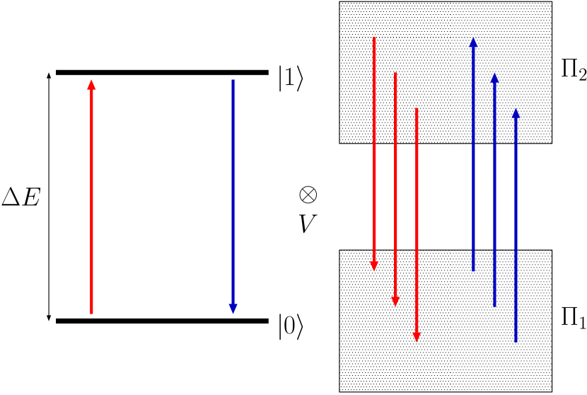
Figure 1: A two-state system which is coupled to an environment consisting of two energy bands.

We employ a projection superoperator of the form BGM

$${\mathcal{P}}\rho = {\mathrm{tr}}_{E}\left\{\Pi_{1}\rho\right\}\otimes\frac{1}{N_{1}}\Pi_{1}+{\mathrm{tr}}_{E}\left\{\Pi_{2}\rho\right\}\otimes\frac{1}{N_{2}}\Pi_{2}$$ (32)

$$\equiv \rho_{1}\otimes\frac{1}{N_{1}}\Pi_{1}+\rho_{2}\otimes\frac{1}{N_{2}}\Pi_{2},$$

where $\Pi_{1}$ ($\Pi_{2}$) denotes the projection onto the lower (upper) environmental energy band. This is a projection of the form given in Eq. (14). It projects onto a state in which the environmental state $\Pi_{i}/N_{i}$ is correlated with the system state $\rho_{i}/{\mathrm{tr}}_{S}\rho_{i}$. The second order of the time-convolutionless projection operator technique leads to the master equation (written in the interaction picture)

$$\frac{d}{dt}\rho_{1} = \gamma_{1}\sigma_{+}\rho_{2}\sigma_{-}-\frac{\gamma_{2}}{2}\{\sigma_{+}\sigma_{-},\rho_{1}\},$$ (33)

$$\frac{d}{dt}\rho_{2} = \gamma_{2}\sigma_{-}\rho_{1}\sigma_{+}-\frac{\gamma_{1}}{2}\{\sigma_{-}\sigma_{+},\rho_{2}\},$$ (34)

where $\gamma_{1,2}=2\pi\lambda^{2}N_{1,2}/\delta\varepsilon$. This is a coupled system of first-order differential equations for the two unnormalized density matrices $\rho_{1}$ and $\rho_{2}$. It can be written in the form of Eq. (30) by taking $H^{i}=0$, $R^{11}=R^{22}=0$, $R^{12}=\sqrt{\gamma_{1}}\sigma_{+}$, and $R^{21}=\sqrt{\gamma_{2}}\sigma_{-}$. As has been demonstrated in Ref. BGM through a comparison with numerical simulations of the full Schrödinger equation, this master equation yields an excellent approximation of the reduced system’s dynamics.

The second term on the right-hand side of Eq. (33) describes changes of $\rho_{1}$ which are due to downward transitions of the two-state system. These are only possible if the lower band of the environment is populated, i. e., if the environment is in the state $\Pi_{1}/N_{1}$ which is correlated with $\rho_{1}$. For this reason the second term of Eq. (33) involves the density $\rho_{1}$. Correspondingly, the first term on the right-hand side of Eq. (33) describes changes of $\rho_{1}$ caused by excitations of the two-state system. Such excitations are only possible if the environment is in the state $\Pi_{2}/N_{2}$ which is correlated with $\rho_{2}$. Therefore, it is the density $\rho_{2}$ that enters the first term of Eq. (33). Analogous statements hold for Eq. (34). Hence, we see that the transitions described by Eqs. (33) and (34) exactly conserve the total number of excitations (see Sec. III.3.2).

Let us investigate the behavior of the excited state population $p_{e}(t)$ which is defined by the expression

$$p_{e}(t)=\langle 1|\rho_{1}(t)+\rho_{2}(t)|1\rangle.$$

Equations (33) and (34) lead to

$$\frac{d}{dt}p_{e}(t) = -(\gamma_{1}+\gamma_{2})p_{e}(t)+\gamma_{1}p_{e}(0)$$ (35)

$$+\gamma_{2}\langle 1|\rho_{2}(0)|1\rangle+\gamma_{1}\langle 0|\rho_{2}(0)|0\rangle.$$

This equation exhibits a strong non-Markovian character because the initial data appear as inhomogeneous terms on its right-hand side. These terms express a pronounced memory effect: They imply that the dynamics never forgets its initial condition, i. e., that the process is governed by an infinite memory time. A further remarkable feature of Eq. (35) derives from the fact that the initial data on its right-hand side cannot be expressed solely in terms of the matrix elements of the reduced density matrix. This means that at any time $t$, and even in the limit $t\rightarrow\infty$, the process is strongly influenced by the statistical correlations of the initial state. Hence, the influence of the initial correlations never dies out and is present even in the stationary state.

Recently, Esposito and Gaspard GASPARD1 ; GASPARD2 have derived a master equation from a microscopic system-reservoir model within second order perturbation theory, which is also of the form of Eq. (30). In their derivation the index $i$ plays the role of the energy $\varepsilon$ of the reservoir. The corresponding density matrix $\rho_{i}\equiv\rho_{\varepsilon}$ describes a system state which is correlated with a certain reservoir state of energy $\varepsilon$. If the open system represents again a two-state system, the master equation of Esposito and Gaspard can be written as

$$\frac{d}{dt}\rho_{\varepsilon} = -i\left[H^{\varepsilon},\rho_{\varepsilon}\right]$$

$$+\sum_{\varepsilon^{\prime}}\left(\gamma_{1}(\varepsilon,\varepsilon^{\prime})\sigma_{+}\rho_{\varepsilon^{\prime}}\sigma_{-}-\frac{\gamma_{2}(\varepsilon^{\prime},\varepsilon)}{2}\left\{\sigma_{+}\sigma_{-},\rho_{\varepsilon}\right\}\right.$$

$$\left.+\gamma_{2}(\varepsilon,\varepsilon^{\prime})\sigma_{-}\rho_{\varepsilon^{\prime}}\sigma_{+}-\frac{\gamma_{1}(\varepsilon^{\prime},\varepsilon)}{2}\left\{\sigma_{-}\sigma_{+},\rho_{\varepsilon}\right\}\right).$$

Here, $\gamma_{1,2}(\varepsilon,\varepsilon^{\prime})$ are certain transition rates which are determined by the parameters of the microscopic model, and $H^{\varepsilon}$ is the system Hamiltonian including an $\varepsilon$-dependent Lamb-type energy renormalization. One easily checks that this master equation can indeed be brought into the general form of Eq. (30) by taking $R_{1}^{\varepsilon\varepsilon^{\prime}}=\sqrt{\gamma_{1}(\varepsilon,\varepsilon^{\prime})}\sigma_{+}$ and $R_{2}^{\varepsilon\varepsilon^{\prime}}=\sqrt{\gamma_{2}(\varepsilon,\varepsilon^{\prime})}\sigma_{-}$.

A master equation of the general form (30) has been derived recently by Budini BUDINI06 . This author suggests introducing an extra degree of freedom $U$ which modulates the interaction between the reduced system $S$ and its environment $E$. Under the assumptions that $E$ may be treated as a Markovian reservoir and that the dynamics of the populations decouples from the dynamics of the coherences of $U$, one arrives at the master equation (30). In a certain sense the introduction of an additional degree of freedom $U$ corresponds to the extended state space ${\mathcal{H}}_{S}\otimes{\mathbb{C}}^{n}$ used in Sec. III.2 to construct the embedding into a Lindblad dynamics. An advantage of the present formulation is that it avoids the use of a microscopic model for the extra degree of freedom and that it clearly shows the basic physical condition underlying the master equation (30): This condition is the existence of an effective representation of the dynamics through a projection onto separable, classically correlated quantum states.

What are the physical conditions under which the use of a standard projection onto a tensor product state is not sufficient to correctly describe the reduced system’s dynamics for a given system-environment model? While this important question seems to be difficult to answer in full generality and certainly deserves further investigations, important hints can be obtained already by an investigation of the time-convolutionless perturbation expansion SHIBATA ; TheWork . If the two-point environmental correlation functions do not decay rapidly in time the second order of the expansion cannot, of course, be expected to give an accurate description of the dynamics. For instance, this situation arises for the spin star model discussed in Ref. BBP , where the second-order generator of the master equation increases linearly with time such that the Born-Markov approximation simply does not exist. The example investigated in Ref. BGM demonstrates that there are even cases in which the standard Markov condition is satisfied although the product-state projection completely fails if one truncates the expansion at any finite order. In such cases strong non-Markovian dynamics is induced through the behavior of higher-order correlation functions. Hence, one can judge the quality of a given projection superoperator only by an investigation of the structure of higher orders of the expansion. The standard projection and the corresponding Lindblad equation are not reliable if higher orders lead to contributions that are not bounded in time, signifying the non-uniform convergence of the perturbation expansion BGM .

III.3.2 Conservation laws and relevant observables

For many physical models one knows certain quantities $C$ which are exactly (or at least approximately) conserved under the time-evolution. A great advantage of the formulation by means of the master equation (30) is that it allows the implementation of the corresponding conservation laws. For instance, the master equation derived in Ref. GASPARD1 reflects the conservation of the (uncoupled) total system energy.

To formulate the conservation of $C$ one chooses the operators $A_{i}$ in such a way that $C$ is a relevant observable [see Sec. II.4]. According to Eq. (16) this means that $C$ can be written in the form

$$C=\sum_{i}C^{i}_{S}\otimes A_{i}.$$

Then we have the exact relation

$${\mathrm{tr}}\{C\rho(t)\}={\mathrm{tr}}\{C{\mathcal{P}}\rho(t)\}=\sum_{i}{\mathrm{tr}}_{S}\{C^{i}_{S}\rho_{i}(t)\}.$$

Hence, we can express the conservation of $C$ on the level of the master equation by means of the conservation law

$$\frac{d}{dt}\sum_{i}{\mathrm{tr}}_{S}\{C^{i}_{S}\rho_{i}(t)\}=0.$$

By use of the master equation (30) this yields a relation between the operators $H^{i}$ and $R^{ij}_{\lambda}$:

$$i\left[H^{i},C^{i}_{S}\right]+\sum_{j\lambda}\left(R^{ji\dagger}_{\lambda}C^{j}_{S}R^{ji}_{\lambda}-\frac{1}{2}\left\{R^{ji\dagger}_{\lambda}R^{ji}_{\lambda},C^{i}_{S}\right\}\right)=0.$$

Thus, known conserved quantities lead to constraints on the choice of the operators that enter the master equation.

An example is given by the quantity $C=\sigma_{+}\sigma_{-}+\Pi_{2}$ which counts the total number of excitations for the model discussed in Sec. III.3.1. This quantity is exactly conserved under the evolution generated by the Hamiltonian (31). Writing

$$C=\sigma_{+}\sigma_{-}\otimes\Pi_{1}+(\sigma_{+}\sigma_{-}+I_{S})\otimes\Pi_{2}$$

we see that $C$ is indeed a relevant observable for the projection (32), i. e., we have ${\mathcal{P}}^{\dagger}C=C$. The corresponding conservation law takes the form

$$p_{e}(t)+{\mathrm{tr}}_{S}\rho_{2}(t)={\mathrm{const.}}$$

This fact can be used to motivate the projection superoperator: With the choice of Eq. (32) one ensures that the projection superoperator leaves invariant the conserved quantity and that the effective description respects the corresponding conservation law.

IV Conclusions

We have discussed the theoretical description of non-Markovian quantum dynamics within the framework of the projection operator techniques. It has been shown that an efficient modelling of strong non-Markovian effects is made possible through the use of correlated projection superoperators ${\mathcal{P}}$ that take into account statistical correlations between the open system and its environment. We have formulated and explained some general physical conditions which demand, essentially, that ${\mathcal{P}}$ can be expressed in terms of a projective quantum channel that operates on the environmental variables. On the basis of these conditions a representation theorem for correlated projection operators [Eq. (12)] has been derived.

Employing a correlated projection superoperator instead of the usual projection onto a tensor product state, one enlarges the set of dynamical variables from the reduced density matrix $\rho_{S}$ to a collection of densities $\rho_{i}$ describing system states that are correlated with certain environmental states. By means of an embedding of the non-Markovian dynamics into a Lindblad dynamics on a suitably extended state space, we have derived the general structure of a master equation [Eq. (30)] which governs the dynamics of the $\rho_{i}$ and models strong non-Markovian effects, while preserving the physical conditions of normalization and positivity. A particularly important feature of the master equation is that it is able to describe very long and even infinite memory times, as well as large correlations in the initial state.

We have also discussed the role of known conserved quantities. Such quantities may be helpful to find an appropriate projection superoperator by demanding that they be relevant observables for ${\mathcal{P}}$. Once this has been achieved one can express the corresponding conservation laws on the level of the effective description provided by the master equation.

The semigroup assumption used in the derivation of the master equation (30) is not really necessary. In fact, the present formulation can easily be extended to the case of an explicitly time-dependent Lindblad generator on the extended state space. The resulting master equation is then again of the form of Eq. (30), where the operators $H^{i}(t)$ and $R_{\lambda}^{ij}(t)$ now depend explicitly on time.

The result expressed by Eq. (30) could be particularly useful for a phenomenological approach to non-Markovian dynamics: For arbitrary $H^{i}$ and $R^{ij}_{\lambda}$ this equation represents a physically acceptable master equation because it preserves the normalization of the reduced density matrix and transforms positive initial components $\rho_{i}(0)\geq 0$ into positive components $\rho_{i}(t)\geq 0$. We emphasize that the argument leading to the form (30) of the master equations is non-perturbative. Given a certain projection superoperator ${\mathcal{P}}$ defining the densities $\rho_{i}$, the only assumption entering the derivation is the existence of an embedding of the dynamics into a Lindblad dynamics on the extended state space.

The projection superoperators used for the description of non-Markovian dynamics in Sec. III have a special feature. Namely, they project any given state onto a classically correlated state. If a non-Markovian dynamics can be approximated by use of such a superoperator within low orders of the perturbation expansion, one can conclude that the true states of the total system can be represented effectively through classically correlated states and that genuine quantum correlations (entanglement) may be treated as perturbations. On the other hand, the representation theorem of Sec. II.2 includes the case of projection superoperators that project onto nonseparable (entangled) quantum states. For such superoperators the arguments that led to the master equation (30) are not applicable. It remains an important open problem to extend the formulation developed here to the case of nonseparable projection superoperators. Such an extension could enable a systematic investigation of the dynamical significance of genuine quantum correlations in non-Markovian processes.

- (1) H. P. Breuer and F. Petruccione, The Theory of Open Quantum Systems (Oxford University Press, Oxford, 2002).
- (2) F. Haake and R. Reibold, Phys. Rev. A 32, 2462 (1985).
- (3) B. L. Hu, J. P. Paz and Y. Zhang, Phys. Rev. D 45, 2843 (1992).
- (4) H. Grabert, P. Schramm, and G.-L. Ingold, Phys. Rep. 168, 115 (1988).
- (5) P. Štelmachovič and V. Bužek, Phys. Rev. A 64, 062106 (2001); Phys. Rev. A 67, 029902(E) (2003).
- (6) J. Schliemann, A. Khaetskii, and D. Loss, J. Phys.: Condens. Matter 15, R1809 (2003).
- (7) J. Gemmer and M. Michel, Europhys. Lett. 73, 1 (2006).
- (8) J. Gemmer, M. Michel, and G. Mahler, Quantum Thermodynamics, Lecture Notes in Physics, Vol. 657 (Springer, Berlin, 2004).
- (9) M. Michel, G. Mahler and J. Gemmer, Phys. Rev. Lett. 95, 180602 (2005).
- (10) S. Nakajima, Progr. Theor. Phys. 20, 948 (1958).
- (11) R. Zwanzig, J. Chem. Phys. 33, 1338 (1960).
- (12) F. Haake, Statistical Treatment of Open Systems, Springer Tracts in Modern Physics, Vol. 66 (Springer, Berlin, 1973).
- (13) R. Kubo, M. Toda, and N. Hashitsume, Statistical Physics II. Nonequilibrium Statistical Mechanics, (Springer, Berlin, 1991).
- (14) F. Shibata, Y. Takahashi, and N. Hashitsume, J. Stat. Phys. 17, 171 (1977); S. Chaturvedi and F. Shibata, Z. Phys. B 35, 297 (1979); F. Shibata and T. Arimitsu, J. Phys. Soc. Jap. 49, 891 (1980); C. Uchiyama and F. Shibata, Phys. Rev. E 60, 2636 (1999); A. Royer, Phys. Lett. A 315, 335 (2003); H. P. Breuer, Phys. Rev. A 70, 012106 (2004).
- (15) V. Gorini, A. Kossakowski, and E. C. G. Sudarshan, J. Math. Phys. 17, 821 (1976).
- (16) G. Lindblad, Commun. Math. Phys. 48, 119 (1976).
- (17) H. Spohn, Rev. Mod. Phys. 53, 569 (1980).
- (18) H. P. Breuer, D. Burgarth, and F. Petruccione, Phys. Rev. B 70, 045323 (2004).
- (19) M. Esposito and P. Gaspard, Phys. Rev. E 68, 066112 (2003).
- (20) M. Esposito and P. Gaspard, Phys. Rev. E 68, 066113 (2003).
- (21) A. A. Budini, Phys. Rev. E 72, 056106 (2005).
- (22) H. P. Breuer, J. Gemmer, and M. Michel, Phys. Rev. E 73, 016139 (2006).
- (23) S. M. Barnett and S. Stenholm, Phys. Rev. A 64, 033808 (2001).
- (24) A. A. Budini, Phys. Rev. A 69, 042107 (2004).
- (25) A. Shabani and D. A. Lidar, Phys. Rev. A 71, 020101(R) (2005).
- (26) S. Maniscalco and F. Petruccione, Phys. Rev. A 73, 012111 (2006).
- (27) V. Gorini, A. Frigerio, M. Verri, A. Kossakowski, and E. C. G. Sudarshan, Rep. Math. Phys. 13, 149 (1978).
- (28) K. Kraus, Ann. Phys. (N.Y.) 64, 311 (1971).
- (29) W. F. Stinespring, Proc. Amer. Math. Soc. 6, 211 (1955).
- (30) G. Alber, T. Beth, M. Horodecki, P. Horodecki, R. Horodecki, M. Rötteler, H. Weinfurter, R. Werner, and A. Zeilinger, Quantum Information (Springer-Verlag, Berlin, 2001).
- (31) R. F. Werner, Phys. Rev. A 40, 4277 (1989).
- (32) A. A. Budini, Phys. Rev. A 74, 053815 (2006).