Intrinsic Quantum Computation

Abstract

We introduce ways to measure information storage in quantum systems, using a recently introduced computation-theoretic model that accounts for measurement effects. The first, the quantum excess entropy, quantifies the shared information between a quantum process’s past and its future. The second, the quantum transient information, determines the difficulty with which an observer comes to know the internal state of a quantum process through measurements. We contrast these with von Neumann entropy and quantum entropy rate and provide a closed-form expression for the latter for the class of deterministic quantum processes.

Poincaré discovered that classical mechanical systems can appear to be random [1]. Kolmogorov, adapting Shannon’s theory of communication [2], showed that their degree of randomness can be measured as a rate of information production [3]. Shannon, in fact, adopted the word “entropy” to describe information transmitted through a communication channel based on a suggestion by von Neumann, who had recently used entropy to describe the distribution of states in quantum systems [4, Ch. 5]. Information has a long history in quantifying degrees of disorder in both classical and quantum mechanical systems.

In a seemingly unrelated effort, Feynman proposed to develop quantum computers [5] with the goal of (greatly) accelerating simulation of quantum systems. Their potential power, though, was brought to the fore most recently by the discovery of algorithms that would run markedly faster on quantum computers than on classical computers. Experimental efforts to find a suitable physical substrate for a quantum computer have been well underway for almost a decade now [6].

In parallel, the study of the quantum behavior of classically chaotic systems gained much interest [7], most recently including the role of measurement. It turns out that measurement interaction leads to genuinely chaotic behavior in quantum systems, even far from the semi-classical limit [8].

How are computing, information creation, and dynamics related? A contemporary view of these three historical threads is that they are not so disparate. We show here that a synthesis leads to methods to analyze how quantum processes store and manipulate information—what we refer to as intrinsic quantum computation.

Computation-theoretic comparisons of classical (stochastic) and measured quantum systems showed that a quantum system’s behavior depends sensitively on how it is measured. The differences were summarized in a hierarchy of computational model classes for quantum processes [9]. Here we adopt an information-theoretic approach that, on the one hand, is more quantitative than and, on the other, is complementary to the structural view emphasized by the computation-theoretic analysis. To start, recall the finite-state quantum generators defined there. They consist of a finite set of internal states $Q=\{q_{i}:i=0,\ldots,|Q|-1\}$. The state vector over the internal states is an element of a $|Q|$-dimensional Hilbert space: $\mathinner{\langle{\psi}|}\in\mathcal{H}$. At each time step a quantum generator outputs a symbol $s\in\mathcal{A}$ and updates its state vector.

The temporal dynamics is governed by a set of $|Q|$-dimensional transition matrices $\{T(s)=U\cdot P(s),s\in\mathcal{A}\}$, whose components are elements of the complex unit disk and where each is a product of a unitary matrix $U$ and a projection operator $P(s)$. $U$ governs the evolution of the state vector. $\mathbf{P}=\{P(s):s\in\mathcal{A}\}$ is a set of projection operators that determine how the state vector is measured. We base our analysis on the class of projective measurements, applicable to closed quantum systems. In the measurement setting used here the output symbol $s$ is identified with the measurement outcome and labels the system’s eigenvalues. We represent the event of no measurement with the symbol $\lambda$; $P(\lambda)$ can be thought of as the identity matrix. Thus, starting with state vector $\mathinner{\langle{{\psi_{0}}}|}$, a single time-step yields $\langle\psi(s)|=\langle\psi_{0}|U\cdot P(s)$.

To describe how an observer chooses to measure a quantum system we introduce the notion of a measurement protocol. A measurement act—applying $P(m),m\in\mathcal{A}\bigcup\lambda$—returns a value $s\in\mathcal{A}$ or nothing ($m=\lambda$). A measurement protocol, then, is a choice of a sequence of measurement acts $m_{t}\in\mathcal{A}\bigcup\lambda$. If an observer asks if the measurement outcomes $s_{1}s_{2}s_{3}$ occur, the answer depends on the measurement protocol, since the observer could choose protocol $s_{1}\lambda\lambda s_{2}\lambda s_{3}$, $s_{1}s_{2}s_{3}$, or others. Fixing a measurement protocol, then, the state vector after observing the measurement series $m^{N}=m_{1}\ldots m_{N}$ is $\langle\psi(m^{N})|=\langle\psi_{0}|U\cdot P(m_{1})\cdot U\cdot P(m_{2})\cdots U\cdot P(m_{N})$.

A quantum process is the joint distribution ${\rm Pr}(\ldots S_{-2}S_{-1}S_{0}S_{1}\ldots)$ over the infinite chain of measurement random variables $S_{t}$. Defined in this way, it is the quantum analog of what Shannon referred to as an information source [10]. Starting a generator in $\langle\psi_{0}|$ the probability of output $s$ is given by the state vector without renormalization: $\mathrm{Pr}(s)=\left\|\psi(s)\right\|^{2}$. By extension, the word distribution, the probability of outcomes $s^{L}$ from a sequence of $L$ measurements, is $\mathrm{Pr}(s^{L})=\left\|\psi(s^{L})\right\|^{2}$.

We can use the observed behavior, as reflected in the word distribution, to come to a number of conclusions about how a quantum process generates randomness and stores and transforms historical information. The Shannon entropy of length-$L$ sequences is defined

$$H(L) \equiv-\sum_{s^{L}\in{\cal A}^{L}}\mathrm{Pr}(s^{L}){\rm log}_{2}\mathrm{Pr}(s^{L})~{}.$$ (1)

It measures the average surprise in observing the “event” $s^{L}$. Ref. [11] showed that a stochastic process’s informational properties can be derived systematically by taking derivatives and then integrals of $H(L)$, as a function of $L$. For example, the source entropy rate $h_{\mu}$ is the rate of increase with respect to $L$ of the Shannon entropy in the large-$L$ limit:

$$h_{\mu}\equiv\lim_{L\rightarrow\infty}\left[H(L)-H(L-1)\right]\;,$$ (2)

where the units are bits/measurement [10]. The entropy rate $h_{\mu}$ quantifies the irreducible randomness in measurement sequences produced by a process: the randomness that remains after the correlations and structures in longer and longer sequences are taken into account. The latter, in turn, are measured by two complementary quantities. The amount $I(\stackrel{{\scriptstyle\leftarrow}}{{S}};\stackrel{{\scriptstyle\rightarrow}}{{S}})$ of mutual information [10] shared between a process’s past $\stackrel{{\scriptstyle\leftarrow}}{{S}}$ and its future $\stackrel{{\scriptstyle\rightarrow}}{{S}}$ is given by the excess entropy ${\bf E}$ [11]. It is the subextensive part of $H(L)$:

$${\bf E}=\lim_{L\rightarrow\infty}[H(L)-h_{\mu}L]\;.$$ (3)

Note that the units here are bits. Ref. [11] also showed that the amount of information an observer must extract from measurements in order to know the internal state is given by the transient information:

$${\bf T}\equiv\sum_{L=0}^{\infty}\left[{\bf E}+h_{\mu}L-H(L)\right]\;,$$ (4)

where the units are bits $\times$ measurements.

If one can determine the word distribution $\mathrm{Pr}(s^{L})$, then, in principle at least, one can calculate a quantum process’s informational properties: $h_{\mu}$, ${\bf E}$, and ${\bf T}$. Fortunately, there are several classes of quantum process for which one can give closed-form expressions. For example, we will provide a way of computing $h_{\mu}$ exactly, using the finite-state machine representation of a quantum process, similar to what is known for classical stochastic processes [12]. We then give examples of various quantum processes at the end, measuring their intrinsic computation.

In quantum theory one distinguishes between complete and incomplete measurements. A complete measurement projects onto a one-dimensional subspace of $\mathcal{H}$. A complete quantum generator (CQG) is simply a quantum generator observed with complete measurements.

Another, as it turns out, more general class of quantum processes are those that can be described by a deterministic quantum generator (DQG), where each matrix $T(s)$ has at most one nonzero entry per row. The importance of determinism comes from the fact that it guarantees that an internal-state sequence $q_{t}q_{t+1}q_{t+2}\ldots$ is in 1-to-1 correspondence with a measurement sequence $s_{t}s_{t+1}s_{t+2}$.

It simplifies matters if the word distribution is independent of the initial state vector $\mathinner{\langle{\psi_{0}}|}$. This is achieved by switching to the density matrix formalism [9]. A stationary state distribution $\rho^{s}$ can then be found for DQGs and $\mathrm{Pr}(s^{L})=\mathrm{Tr}\left[T^{\dagger}(s^{L})\rho^{s}T(s^{L})\right]$ is start-state independent.

We showed that every DQG has an equivalent deterministic classical generator that produces the same stochastic process [9]. Specifically, given a DQG $M=\{U,P(s)\}$, the equivalent classical generator $M^{\prime}=\{T,P(s)\}$ has unistochastic transition matrix $T_{ij}=|U_{ij}|^{2}$.

As a consequence, when a quantum process can be represented by a complete or a deterministic generator, closed-form expressions exist for several of the information quantities. For example, adapting Ref. [12] to DQGs we obtain the quantum entropy rate:

$$h_{\mu}=-|Q|^{-1}\sum_{i=0}^{|Q|-1}\sum_{j=0}^{|Q|-1}|U_{ij}|^{2}\log_{2}|U_{ij}|^{2}~{},$$ (5)

using the fact that $\rho^{s}_{ii}=|Q|^{-1}$ for DQGs. This should be compared to the entropy rates for nondeterministic classical and quantum processes which, in general, have no closed-form expression. For DQGs we introduce the internal-state quantum entropy:

$$S_{q}=-\sum_{i=0}^{|Q|-1}\rho^{s}_{ii}\log_{2}\rho^{s}_{ii}~{},$$ (6)

which measures the average uncertainty in knowing the internal state. Again, $\rho_{ii}=|Q|^{-1}$ for DQGs allows us to simplify: $S_{q}=\log_{2}|Q|$.

$S_{q}$, as defined here, is nothing other than the von Neumann entropy $S(\rho)$ of the density matrix $\rho$ [13]. Note, that our use of the density matrix is as a time average, not an ensemble average. This should be further compared to the von Neumann entropy $S(\otimes_{i=0}^{L-1}\rho_{i})$ over a sequence of density matrices produced by a stationary quantum source [14]. Using this, a density-matrix quantum entropy rate can be defined as the limit of $S(\otimes_{i=0}^{L-1}\rho_{i})/L$ for large $L$. Note that these alternative definitions of entropy and entropy rate suffer from two problems. First, they refer to internal variables that are not directly measurable. Second, they do not take the effects of measurement into account. Importantly, $h_{\mu}$, ${\bf E}$, and ${\bf T}$ do not suffer from these problems. Let’s explore their consequences for characterizing intrinsic computation in several simple quantum dynamical systems. (An exhaustive analysis of all (deterministic and non-deterministic) few-qubit quantum processes will appear elsewhere.)

The iterated beam-splitter (Fig. 1) is a quantum system that, despite its simplicity, makes a direct connection to familiar experiments. Photons are sent through a beam-splitter, producing two possible paths, which are redirected by mirrors and recombined at the beam-splitter after passing around the feedback loop determined by the mirrors. Nondestructive detectors are located along the upper and lower paths.

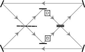
Figure 1: Iterated beam splitter: Thick solid lines are mirrors. Photon detectors, marked as D, are placed in upper and lower photon paths (solid gray lines).

The iterated beam splitter is a quantum dynamical system with a two-dimensional state space (which path is taken around the loop) with eigenstates “above” $\mathinner{\langle{{\phi_{A}}}|}$ and “below”$\mathinner{\langle{{\phi_{B}}}|}$. Its dynamics are given by a unitary operator for the beam-splitter, the Hadamard matrix $U_{H}=\tfrac{1}{\sqrt{2}}\left(\begin{smallmatrix}1&1\\ 1&-1\end{smallmatrix}\right)$, and measurement operators representing the detectors: $P(0)=\mathinner{|{0}\rangle}\mathinner{\langle{0}|}$ and $P(1)=\mathinner{|{1}\rangle}\mathinner{\langle{1}|}$, in the experiment’s eigenbasis. Measurement symbol $0$ stands for “above” and symbol $1$ stands for “below”.

The detectors after the first beam splitter detect the photon in the upper or lower path with equal probability. Once the photon is measured, though, it is in that detector’s path with probability $1$. And so it enters the beam splitter again in the same state as when it first entered. Thus, the measurement outcome after the second beam splitter will have the same uncertainty as after the first: the detectors still report “above” or “below” with equal probability. The resulting sequence of detector outcomes after many circuits of the feedback loop is simply a random sequence. Call this measurement protocol I.

Now alter the experiment slightly by activating the detectors only after every other circuit of the feedback loop. In this set-up, call it protocol II, the photon enters the first beam splitter, passes an inactive detector and interferes with itself when it returns to the beam splitter. This, as we will confirm, leads to destructive interference of one path after the beam splitter. The photon is thus in the same path after the second visit to the beam splitter as it was on the first. The now-active detector therefore reports with probability $1$ that the photon is in the upper path, if the photon was initially in the upper path. If it was initially in the lower path, then the detector reports that it is in the upper path with probability $0$. The resulting sequence of path detections is a very predictable sequence, compared to the random sequence from protocol I. Note that both protocols are complete measurements.

We now construct a complete quantum generator for the iterated-beam splitter. The output alphabet consists of two symbols denoting detection “above” or “below”: $\mathcal{A}=\{0,1\}$. There are two internal states “above” and “below”, each associated with one of the two system eigenstates: $Q=\{A,B\}$. The transition matrices are $T(0)=U_{H}P(0)$ and $T(1)=U_{H}P(1)$. We assume that the quantum process has been operating for some time and so take $\rho^{s}=|Q|^{-1}\sum_{i\in Q}\mathinner{|{\phi_{i}}\rangle}\mathinner{\langle{\phi_{i}}|}$.

One can readily verify that this representation of the iterated beam splitter is a DQG. And so we can determine its classical equivalent generator has transition matrices $T(0)=\frac{1}{2}\left(\begin{smallmatrix}1&0\\ 1&0\end{smallmatrix}\right)~{}\mathrm{and}~{}T(1)=\frac{1}{2}\left(\begin{smallmatrix}0&1\\ 0&1\end{smallmatrix}\right)$. The sequences it generates for protocol I are described by the uniform distribution at all lengths: $\mathrm{Pr}(s^{L})=2^{-L}$.

Note, however, that the probability distribution of the sequences for the classical generator under protocol II is still the uniform distribution for all lengths $L$. This could not be more different from the behavior of the (quantum) iterated beam splitter under protocol II. The classical generator is simply unable to capture the interference effects present in this case. A second classical generator must be constructed from the quantum generator’s transition matrices for protocol II. One finds $T(0)=\tfrac{1}{2}\left(\begin{smallmatrix}1&0\\ 0&0\end{smallmatrix}\right)~{}\mathrm{and}~{}T(1)=\tfrac{1}{2}\left(\begin{smallmatrix}0&0\\ 0&1\end{smallmatrix}\right)$. Starting the photon in the upper path again, for protocol II one finds $\mathrm{Pr}(00\ldots)=\mathrm{Pr}(11\ldots)=1/2$ and all other words have zero probability.

Table 1 gives the informational quantities for the iterated beam splitter under the protocols. Under protocol I it is maximally random ($h_{\mu}=1$), as expected. It also, according to ${\bf E}=0$, does not store any historical information and the observer comes to know this immediately (${\bf T}=0$). In stark contrast, under protocol II, the iterated beam splitter is quite predictable ($h_{\mu}=0$) and stores one bit of information (${\bf E}=1$)—whether the measurement sequence is $000\ldots$ or $111\ldots$. Learning which requires extracting one bit (${\bf T}=1$) of information from the measurements.

Note that the internal-state (von Neumann) entropy $S_{q}=1$ under both protocols: there are two equally likely states in both cases. It simply reflects the single qubit in the iterated beam splitter, not whether that qubit is useful in supporting intrinsic computation.

Quantum	Iterated Beam		Spin-1
Dynamical System	Splitter		Particle
Protocol	I	II	I	II
$h_{\mu}$ [bits/measurement]	1	0	0.666	0.666
$S_{q}$ [bits]	1	1	1.585	1.585
${\bf E}$ [bits]	0	1	0.252	0.902
${\bf T}$ [bits$\times$measurement]	0	1	0.252	3.03

Table 1: Information storage and generation for example quantum processes: entropy rate $h_{\mu}$, internal-state entropy $S_{q}$, excess entropy ${\bf E}$, and transient information ${\bf T}$.

Now consider a second, more complex example: A spin-$1$ particle subject to a magnetic field that rotates its spin. The state evolution can be described by the unitary matrix $U=\left(\begin{smallmatrix}1/\sqrt{2}&1/\sqrt{2}&0\\ 0&0&-1\\ -1/\sqrt{2}&1/\sqrt{2}&0\end{smallmatrix}\right)$, which is a rotation in $\mathbb{R}^{3}$ around the y-axis by angle $\tfrac{\pi}{4}$ followed by a rotation around the x-axis by $\tfrac{\pi}{2}$.

Using a suitable representation of the spin operators $J_{i}$ [15, p.199], such as: $J_{x}=\left(\begin{smallmatrix}0&0&0\\ 0&0&i\\ 0&-i&0\end{smallmatrix}\right)$, $J_{y}=\left(\begin{smallmatrix}0&0&i\\ 0&0&0\\ -i&0&0\end{smallmatrix}\right)$, and $J_{z}=\left(\begin{smallmatrix}0&i&0\\ -i&0&0\\ 0&0&0\end{smallmatrix}\right),$ the relation $P_{i}=1-J_{i}^{2}$ defines a one-to-one correspondence between the projector $P_{i}$ and the square of the spin component along the $i$-axis. The resulting measurement poses the yes-no question, Is the square of the spin component along the $i$-axis zero?

Define two protocols, this time differing in the projection operators. First, consider measuring $J_{y}^{2}$; call this protocol I. Then $U$ and the projection operators $P(0)=\mathinner{|{100}\rangle}\mathinner{\langle{100}|}+\mathinner{|{001}\rangle}\mathinner{\langle{001}|}$ and $P(1)=\mathinner{|{010}\rangle}\mathinner{\langle{010}|}$ define a quantum generator.

The stochastic language produced by this process is the so-called Golden-Mean Process language [11]. It is defined by the set of irreducible forbidden words $\mathcal{F}=\{00\}$. That is, all measurement sequences occur, except for those with consecutive $0$s. For the spin-$1$ particle this means that the spin component along the y-axis never equals 0 twice in a row. We call this short-range correlation since there is a correlation between a measurement outcome at time $t$ and the immediately preceding one at time $t-1$. If the outcome is $0$, the next outcome will be $1$ with certainty. If the outcome is $1$, the next measurement is maximally uncertain: outcomes $0$ and $1$ occur with equal probability.

Second, consider measuring the observable $J_{x}^{2}$; call this protocol II. Then $U$ and $P(0)=\mathinner{|{100}\rangle}\mathinner{\langle{100}|}$ and $P(1)=\mathinner{|{010}\rangle}\mathinner{\langle{010}|}+\mathinner{|{001}\rangle}\mathinner{\langle{001}|}$ define a quantum finite-state generator. The stochastic language generated is the Even Process language [11]. It is characterized by an infinite set of irreducible forbidden words $\mathcal{F}=\{01^{2k-1}0\},k=1,2,3,...$. That is, if the spin component equals $0$ along the $x$-axis, it will be zero an arbitrary large, even number of consecutive measurements before being observed to be nonzero.

Table 1 gives the intrinsic-computation analysis of the spin-$1$ system. Comparing it to the iterated beam splitter, it’s clear that the spin-$1$ system is richer—a process that does not neatly fall into one or the other extreme of exactly predictable and utterly unpredictable. In fact, under protocols I and II it appears equally unpredictable: $h_{\mu}\approx 0.333$. As before the von Neumann entropy is also the same under both protocols. The amount of information that the spin-$1$ system communicates from the past to the future is nonzero, with the amount under protocol I (${\bf E}\approx 0.252$) being less than under protocol II (${\bf E}\approx 0.902$). These accord with our observation that in the latter case there is a kind of infinite-range temporal correlation. Not too much information (${\bf T}\approx 0.252$) must be extracted by the observer under protocol I in order to see the relatively little memory stored in this process. Interestingly, however, under protocol II this is markedly larger (${\bf T}\approx 3.03$), indicating again that the observer must extract more information to see just how this process is monitoring “evenness”.

We close by looking at a repeatedly measured quantum system in the context of recent developments in quantum computation. Quantum control theory—a paradigm of repeated classical-state measurement and feedback control—has only recently been implemented as a means to drive quantum systems toward a desired state or dynamic [16]. Current implementations are finite-dimensional and aim at the control of a known quantum state. Therefore, our formalism can be used to characterize the intrinsic computation of these quantum systems. In fact, it can be used on any quantum system observed over time, whether its exact state is known or not. If it is known and the applied measurement protocol generates a deterministic quantum process the above measures of intrinsic computation can be calculated exactly using its quantum generator representation. Generally, though, the intrinsic quantum computation of an unknown quantum state can be measured experimentally by recording a time series of measurement outcomes and computing the probability distribution. In fact, from the probability distribution of a discrete time series of measurements one can compute the intrinsic computation of both open and closed quantum systems.

We introduced several new information-theoretic quantities that reflect a quantum process’s intrinsic computation: its information production rate, how much memory it apparently stores in generating information, and how hard it is for an observer to synchronize. We discussed how several of these informational quantities are related to existing notions of entropy in quantum theory. The contrast allowed us to demonstrate how much more they tell one about the intrinsic computation supported by quantum processes and to highlight the crucial role of measurement. For example, simply knowing that a quantum process is built out of some number of qubits only gives an upper bound on the possible information processing. It does not reflect how the quantum system actually uses the qubits to process information nor how much of its information processing can be observed. For these, one needs the quantum $h_{\mu}$, ${\bf E}$, and ${\bf T}$.

UCD and the Santa Fe Institute supported this work via the Network Dynamics Program funded by Intel Corporation. The Wenner-Gren Foundations, Stockholm, Sweden, provided KW’s postdoctoral fellowship.

References

- [1] H. Poincaré. Les Methodes Nouvelles de la Mecanique Celeste. Gauthier-Villars, Paris, 1892.
- [2] C. E. Shannon. Bell Sys. Tech. J., 27:379–423, 623–656, 1948.
- [3] A. N. Kolmogorov. Dokl. Akad. Nauk. SSSR, 124:754, 1959. (Russian) Math. Rev. vol. 21, no. 2035b.
- [4] J. von Neumann. Mathematical Foundations of Quantum Mechanics. Princeton University Press, Berlin, 1932.
- [5] R. P. Feynman. Intl. J. Theo. Phys., 21:467–488, 1982.
- [6] P. Zoller et al. Euro. Phys. J. D, 36(2):203–228, 2005.
- [7] L. E. Reichl. The transition to chaos: Conservative classical systems and quantum manifestations. Springer, New York, 2004.
- [8] S. Habib, K. Jacobs, and K. Shizume. Phys. Rev. Lett., 96:010403–06, 2006.
- [9] K. Wiesner and J. P. Crutchfield. http://arxiv.org/ abs/quant-ph/0608206, 2006.
- [10] T. Cover and J. Thomas. Elements of Information Theory. Wiley-Interscience, 1991.
- [11] J. P. Crutchfield and D. P. Feldman. Chaos, 13:25 – 54, 2003.
- [12] J. P. Crutchfield and D. P. Feldman. Phys. Rev. E, 55(2):1239R–1243R, 1997.
- [13] M. A. Nielsen and I. L. Chuang. Quantum computation and quantum information. Cambridge University Press, 2000.
- [14] A. Wehrl. Rev. Mod. Phys., 50(2):221–260, Apr 1978.
- [15] A. Peres. Quantum theory: concepts and methods. Kluwer Academic Publishers, Dordrecht, 1993.
- [16] J. M. Geremia, J. K. Stockton, and H. Mabuchi. Science, 304:270–A273, 2004.
- [17] J. E. Hopcroft, R. Motwani, and J. D. Ullman. Introduction to Automata Theory, Languages, and Computation. Addison-Wesley, 2001.