A case concerning the improved transition probability

Abstract

As is well known, the existed perturbation theory can be applied to calculations of energy, state and transition probability in many quantum systems. However, there are different paths and methods to improve its calculation precision and efficiency in our view. According to an improved scheme of perturbation theory proposed by [An Min Wang, quant-ph/0602055 v7], we reconsider the transition probability and perturbed energy for a Hydrogen atom in a constant magnetic field. We find the results obtained by using Wang’s scheme are indeed more satisfying in the calculation precision and efficiency. Therefore, Wang’s scheme can be thought of as a powerful tool in the perturbation calculation of quantum systems.

I Introduction

The traditional method of perturbation theory tells us to calculate the energy and expansion coefficient step by step. That is, we should first calculate the zeroth order energy and wave function, and then the first,the second, and so on. In fact, it is easy to see that such a way introduces the approximation too early, and each order calculation of energy and expansion coefficient of wave function are based on the result of the former orders. After careful examination, we find that the traditional way does not consider the astringency of the expansion of the wave function. There is every possibility that if we reconsider the astringency, the result might be different. In fact, this is effectively embodied in Wang’s scheme of perturbation theory wang1 . In this reference, the author did not introduce approximation until very late, and consider subtly and systemically the affection of high-order approximation to the low-order one. This finally results in a different formalism of expression of perturbed solution of dynamics, and its expansion coefficients contain reasonably the high-order energy amendment.

It can been seen that some physics expressions were modified according to Ref. wang1 and further applications can be expected. This leads us to think that it is important and interesting to consider their influences on the physical problems via first reexamining those familiar and standard examples, and then studying more practical systems, because better precision, higher efficiency, as well as correct physical features are always the aims that physics pursues continuously. Here, we focus our attention on a typical example, which shows satisfying results in the calculation precision, efficient as well as the corresponding physical features. This implies, in our view, that Wang’s scheme of perturbation theory is a powerful tool in the perturbative calculation of quantum system.

In this paper, we intend to study the revisions on transition probability in Ref. wang1 , which is different from traditional one. We find that Wang’s revision to the existed expression of transition probability is never trivial, and we illustrate this conclusion via calculating this revision for a Hydrogen atom in a constant magnetic field. This example concerns the ground state hyperfine structure of Hydrogen atom whose correction of electron self-energy has been studied (see self ), so does similar problem about muonium (see nio and liu ). By comparing our result of transition probability with traditional one, our above view is verified. After referring to the exact solution of this problem, we will see that the improved transition probability given by wang1 does show some of its advantages. From this case it is necessary to realize that perhaps there are also some other problems that need similar revisions in transition probability. We are sure that applications of Wang’s scheme of perturbation theory to other problems should not be unimportant and short of practical significance, although his scheme just contains the higher order revisions.

To effectively organize this article, we divide it into the following main parts. Besides Sec. I which is an introduction, in Sec. II we first introduce the amendment to the transition probability based on the results of wang1 . Next, in Sec. III we provide the calculation of energy of our example according to the Wang’s scheme, then compare it with the exact result, and these results are helpful for us later to calculate the transition probability. Then, in Sec. IV we will take use of Sec.II and Sec.III to calculate the referred case. Finally, in Sec. V we summarize our conclusions and make some discussions.

II Improved TRANSITION PROBABILITY

Let us start with Wang’s scheme of perturbation theory wang1 , denoting the state vector by

$$\mbox{$\left|{\Psi(t)}\right\rangle$}=\sum_{l=0}^{\infty}\sum_{\gamma}c_{\gamma,I}^{(l)}(t)\mbox{$\left|{\phi^{\gamma}}\right\rangle$},$$ (1)

where $\left|{\Psi(t)}\right\rangle$ is the eigenvector of ${H}$, and $\left|{\phi^{\gamma}}\right\rangle$ is the eigenvector of ${H_{0}}$. According to the improved form of the perturbed solution of dynamics in wang1 , the first order amendment of coefficient of state vector is deduced as

$$c_{\gamma,I}^{(1)}(t)=\frac{g_{1}^{\gamma\beta}}{E_{\gamma}-E_{\beta}}\left(1-e^{i\widetilde{\omega}_{\gamma\beta}t}\right),$$ (2)

where $E_{\gamma}$ are eigenvalues of $H_{0}$ with the eigenvector $\left|{\phi^{\gamma}}\right\rangle$, $g_{1}^{\gamma\beta}$ ($\gamma\neq\beta$) are off-diagonal elements of $H_{1}$ in the representation of $H_{0}$, that is $g_{1}^{\gamma\beta}=\mbox{$\left\langle{\phi_{\gamma}}\right|$}H_{1}\mbox{$\left|{\phi_{\beta}}\right\rangle$}$, and

$$\widetilde{\omega}_{\gamma\beta}=\widetilde{E_{\gamma}}-\widetilde{E_{\beta}},$$ (3)

while $\widetilde{E_{\gamma}}$ is so-called improved form of perturbed energy defined by

$$\widetilde{E_{\gamma}}=E_{\gamma}+h_{1}^{\gamma}+G_{\gamma}^{(2)}+G_{\gamma}^{(3)}+G_{\gamma}^{(4)}+\cdots.$$ (4)

Here, $h_{1}^{\gamma}$ are diagonal elements of $H_{1}$ in the representation of $H_{0}$, and

$$G_{\beta}^{(2)}=\sum_{{\beta}_{1}}\frac{1}{E_{\beta}-E_{{\beta}_{1}}}g_{1}^{\beta{\beta}_{1}}g_{1}^{{\beta}_{1}\beta},$$ (5)

$$G_{\beta}^{(3)}=\sum_{{\beta}_{1},{\beta}_{2}}\frac{1}{(E_{\beta}-E_{{\beta}_{1}})(E_{\beta}-E_{{\beta}_{2}})}g_{1}^{\beta{\beta}_{1}}g_{1}^{{\beta}_{1}{\beta}_{2}}g_{1}^{{\beta}_{2}\beta},$$ (6)

$$G_{\beta}^{(4)}=\sum_{{\beta}_{1},{\beta}_{2},{\beta}_{3}}\frac{g_{1}^{\beta{\beta}_{1}}g_{1}^{{\beta}_{1}{\beta}_{2}}g_{1}^{{\beta}_{2}{\beta}_{3}}g_{1}^{{\beta}_{3}\beta}\eta_{\beta{\beta}_{2}}}{(E_{\beta}-E_{{\beta}_{1}})(E_{\beta}-E_{{\beta}_{2}})(E_{\beta}-E_{{\beta}_{3}})}\\ -\sum_{{\beta}_{1},{\beta}_{2}}\frac{g_{1}^{\beta{\beta}_{1}}g_{1}^{{\beta}_{1}\beta}g_{1}^{\beta{\beta}_{2}}g_{1}^{{\beta}_{2}\beta}}{{(E_{\beta}-E_{{\beta}_{1}})}^{2}(E_{\beta}-E_{{\beta}_{2}})},$$ (7)

where $\eta_{\beta{\beta}_{2}}=1-\delta_{\beta{\beta}_{2}}$, and $\eta_{\beta{\beta}_{2}}=0$, if $\beta={\beta}_{2}$; $\eta_{\beta{\beta}_{2}}\neq 0$, if $\beta\neq{\beta}_{2}$. Thus it leads to so-called improved transition probability that is different from the traditional one, that is

$$P_{I}^{\gamma\beta}(t)=\left|g_{1}^{\gamma\beta}\right|^{2}\frac{\sin^{2}(\widetilde{\omega}_{\gamma\beta}t/2)}{(\omega_{\gamma\beta}/2)^{2}}.$$ (8)

III Revision of perturbed ENERGY

Now we begin to study such a system in which a Hydrogen atom is placed in a uniform constant magnetic field, which is in the $+z$ direction in the rectangular coordinate system. Suppose that the atom is at the ground state, thus its Hamiltonian (see Ref. codata Appendix(D1)) is

$${H}={H_{0}}+{H_{1}}\\ =B(\mu_{e}\sigma_{ez}-\mu_{p}\sigma_{pz})+W{{\bm{\sigma}}_{e}}\cdot{{\bm{\sigma}}_{p}}.$$ (9)

In the equation above, we change some symbols that are different from the equation (D1) in Ref. codata . $B$ is the magnitude of magnetic field. $W$ is a coupling constant, and we will give its value later in Sec. IV. $\mu_{e}$ is the electron magnetic moment. $\mu_{p}$ is the magnetic moment of a proton, and ${\bm{\sigma}}=(\sigma_{x},\sigma_{y},\sigma_{z})$ is the Pauli operator. Since it is well known that $\mu_{p}\ll\mu_{e}$, we can easily omit the $B\mu_{p}\sigma_{pz}$ in the ${H}$. Therefore, the division of Hamiltonian can be written as

$${H}={H_{0}}+{H_{1}}=B\mu_{e}\sigma_{ez}+W{{\bm{\sigma}}_{e}}\cdot{{\bm{\sigma}}_{p}}.$$ (10)

Here, ${H_{0}}=W{{\bm{\sigma}}_{e}}\cdot{{\bm{\sigma}}_{p}}$ is the unperturbed part, and ${H_{1}}=B\mu_{e}\sigma_{ez}$ is taken as the perturbed part.

Now we refer to the way proposed by Wang in Ref. wang1 . First, we should calculate the eigenvalues and eigenvectors of ${H_{0}}$. It is easy since we know that ${H_{0}}$ is just the coupling of spins of electron and proton. Here we just list the results and omit the process of calculating them.

$$\quad\mbox{Eigenvalue:}\quad W\Longrightarrow\quad\mbox{Eigenvectors:}\quad\left\{\begin{array}[]{r@{\quad= \quad}l}\phi_{1}&\alpha(e)\alpha(p)\\[8.0pt] \phi_{2}&\frac{1}{\sqrt{2}}[\alpha(e)\beta(p)+\beta(e)\alpha(p)]\\[8.0pt] \phi_{3}&\beta(e)\beta(p)\end{array}\right.,$$ (11)

and

$$\quad\mbox{Eigenvalue:}\quad-3W\Longrightarrow\quad\mbox{Eigenstate:}\quad\phi_{4}\,=\,\frac{1}{\sqrt{2}}[\alpha(e)\beta(p)-\beta(e)\alpha(p)]$$ (12)

Here, $\alpha$ and $\beta$ mean:

$$\alpha=\begin{pmatrix}1\\ 0\end{pmatrix}$$ (13)

$$\beta=\begin{pmatrix}0\\ 1\end{pmatrix}$$ (14)

It is clear that there is a three-fold degeneracy subspace.

Considering that

$$\sigma_{ez}\mbox{$\left|{\phi_{1}}\right\rangle$}=\mbox{$\left|{\phi_{1}}\right\rangle$},\quad\sigma_{ez}\mbox{$\left|{\phi_{2}}\right\rangle$}=\mbox{$\left|{\phi_{4}}\right\rangle$},\quad\sigma_{ez}\mbox{$\left|{\phi_{3}}\right\rangle$}=-\mbox{$\left|{\phi_{3}}\right\rangle$},\quad\sigma_{ez}\mbox{$\left|{\phi_{4}}\right\rangle$}=\mbox{$\left|{\phi_{2}}\right\rangle$}$$ (15)

The ${H}$ matrix in the representation of $H_{0}$ can be written as following :

$${H}=\begin{pmatrix}W+B\mu_{e}&0&0&0\\ 0&W&0&B\mu_{e}\\ 0&0&W-B\mu_{e}&0\\ 0&B\mu_{e}&0&-3W\end{pmatrix}$$ (16)

According to Ref. wang1 , we should redivide ${H}$ into two parts: the diagonal part ${H_{0}^{\prime}}$ and the off-diagonal part ${g_{1}}$, that is,

$${H_{0}^{\prime}}=\begin{pmatrix}W+B\mu_{e}&0&0&0\\ 0&W&0&\\ 0&0&W-B\mu_{e}&0\\ 0&0&0&-3W\end{pmatrix}$$ (17)

$${g_{1}}=\begin{pmatrix}0&0&0&0\\ 0&0&0&B\mu_{e}\\ 0&0&0&0\\ 0&B\mu_{e}&0&0\end{pmatrix}$$ (18)

It is clear that the degeneracy is completely removed by the redivision skill wang1 .

Again from Ref. wang1 , we have

$$\widetilde{E_{\beta}}=(H_{0}^{\prime})_{\beta\beta}+G_{\beta}^{(2)}+G_{\beta}^{(3)}+G_{\beta}^{(4)}+\cdots$$ (19)

Note that $(H_{0}^{\prime})_{\beta\beta}=E_{\beta}+h_{1}^{\beta}$. Thus, using the given matrix above, it is easy to obtain that:

$$G_{1}^{(2)}=G_{1}^{(3)}=G_{1}^{(4)}=0,$$ (20)

$$G_{2}^{(2)}=\frac{{(B{\mu}_{e})}^{2}}{4W},\quad G_{2}^{(3)}=0,\quad G_{2}^{(4)}=-\frac{{(B{\mu}_{e})}^{4}}{(4W)^{3}}$$ (21)

$$G_{3}^{(2)}=G_{3}^{(3)}=G_{3}^{(4)}=0,$$ (22)

$$G_{4}^{(2)}=-\frac{{(B{\mu}_{e})}^{2}}{4W},\quad G_{4}^{(3)}=0,\quad G_{4}^{(4)}=\frac{{(B{\mu}_{e})}^{4}}{(4W)^{3}}$$ (23)

Thus

$$\widetilde{E_{1}} = W+B{\mu}_{e},$$ (24)

$$\widetilde{E_{2}} = W+\frac{{(B{\mu}_{e})}^{2}}{4W}-\frac{{(B{\mu}_{e})}^{4}}{(4W)^{3}},$$ (25)

$$\widetilde{E_{3}} = W-B{\mu}_{e},$$ (26)

$$\widetilde{E_{4}} = -3W-\frac{{(B{\mu}_{e})}^{2}}{4W}+\frac{{(B{\mu}_{e})}^{4}}{(4W)^{3}}.$$ (27)

Since this example can be, in fact, solved exactly, the results above obtained via the perturbation theory can be compared with the exact solution of energy. In terms of the standard method, we immediately get the exact solution of eigenvalues and their corresponding eigenvectors

$$E_{1}^{T}=W+B\mu_{e},\,\Longrightarrow\Psi_{1}=\phi_{1}$$ (28)

$$E_{2}^{T}=-W+\sqrt{4W^{2}+(\mu_{e}B)^{2}},\,\Longrightarrow\Psi_{2}=\frac{1}{\sqrt{(\omega_{42}+\omega_{42}^{T})^{2}+4(\mu_{e}B)^{2}}}\left[(\omega_{42}+\omega_{42}^{T})\phi_{2}-2B\mu_{e}\phi_{4}\right]$$ (29)

$$E_{3}^{T}=W-B\mu_{e}\;\Longrightarrow\Psi_{3}=\phi_{3}$$ (30)

$$E_{4}^{T}=-W-\sqrt{4W^{2}+(\mu_{e}B)^{2}},\,\Longrightarrow\Psi_{4}=\frac{1}{\sqrt{(\omega_{42}-\omega_{42}^{T})^{2}+4(\mu_{e}B)^{2}}}\left[(\omega_{42}-\omega_{42}^{T})\phi_{2}-2B\mu_{e}\phi_{4}\right]$$ (31)

Here $\omega_{42}=E_{4}-E_{2}$, and $\omega_{42}^{T}=E_{4}^{T}-E_{2}^{T}$.

When the magnitude of magnetic field $B$ is very weak, we can expand the exact result of energy, which can be compared with the energy worked out by the new way. Assuming that $B\mu_{e}\ll W$, thus

$$E_{2}^{T} = -W+2W\left(1+\frac{(B\mu_{e})^{2}}{4W^{2}}\right)^{\frac{1}{2}}$$ (32)

$$= -W+2W\left[1+\frac{(B\mu_{e})^{2}}{8W^{2}}-\frac{(B\mu_{e})^{4}}{8(4W^{2})^{2}}+\cdots\right]$$

$$\approx W+\frac{(B{\mu_{e}})^{2}}{4W}-\frac{(B\mu_{e})^{4}}{(4W)^{3}}$$

$$= \widetilde{E_{2}}$$

$$E_{4}^{T} = -W-2W\left(1+\frac{(B\mu_{e})^{2}}{4W^{2}}\right)^{\frac{1}{2}}$$ (33)

$$= -W-2W\left[1+\frac{(B\mu_{e})^{2}}{8W^{2}}-\frac{(B\mu_{e})^{4}}{8(4W^{2})^{2}}+\cdots\right]$$

$$\approx -3W-\frac{(B{\mu_{e}})^{2}}{4W}+\frac{(B\mu_{e})^{4}}{(4W)^{3}}$$

$$= \widetilde{E_{4}}$$

while

$$E_{1}^{T}=\widetilde{E_{1}},\quad E_{3}^{T}=\widetilde{E_{3}}.$$ (34)

Obviously, we see that the perturbed energy calculated by using Wang’s scheme wang1 is more satisfying because they have better precision than the existed method when two kinds of results are compared with the exact results.

IV Calculation of IMPROVED TRANSITION PROBABILITY

In this section we will consider the transition probability from the state $\left|{\phi_{2}}\right\rangle$ to state $\left|{\phi_{4}}\right\rangle$. First, we should calculate its exact result. Obviously the transition probability is:

$$P^{T}(2\to 4)=\left|\mbox{$\left\langle{\phi_{4}}\right|$}e^{-i{H}t}\mbox{$\left|{\phi_{2}}\right\rangle$}\right|^{2}$$ (35)

To work out this equation, we take use of the completeness of the Hilbert space $\{\mbox{$\left|{\Psi_{1}}\right\rangle$},\mbox{$\left|{\Psi_{2}}\right\rangle$},\mbox{$\left|{\Psi_{3}}\right\rangle$},\mbox{$\left|{\Psi_{4}}\right\rangle$}\}$ given above, which means:

$$\begin{array}[]{lll}P^{T}(2\to 4)&=&\left|\sum_{\gamma_{1},\gamma_{2}=1}^{4}\mbox{$\left\langle{\phi_{4}}\right|$}\mbox{$\left|{\Psi_{\gamma_{1}}}\right\rangle$}\mbox{$\left\langle{\Psi_{\gamma_{1}}}\right|$}e^{-i{H}t}\mbox{$\left|{\Psi_{\gamma_{2}}}\right\rangle$}\mbox{$\left\langle{\Psi_{\gamma_{2}}}\right|$}\mbox{$\left|{\phi_{2}}\right\rangle$}\right|^{2}\\ &=&\left|\mbox{$\left\langle{\phi_{4}}\right|$}\mbox{$\left|{\Psi_{2}}\right\rangle$}\mbox{$\left\langle{\Psi_{2}}\right|$}\mbox{$\left|{\phi_{2}}\right\rangle$}e^{-iE^{T}_{2}t}+\mbox{$\left\langle{\phi_{4}}\right|$}\mbox{$\left|{\Psi_{4}}\right\rangle$}\mbox{$\left\langle{\Psi_{4}}\right|$}\mbox{$\left|{\phi_{2}}\right\rangle$}e^{-iE^{T}_{4}t}\right|^{2}\\ &=&(\mu_{e}B)^{2}\dfrac{\sin^{2}(\omega_{42}^{T}t/2)}{(\omega_{42}^{T}/2)^{2}}\end{array}$$ (36)

where $\displaystyle\omega^{T}_{42}=E^{T}_{4}-E^{T}_{2}=-2\sqrt{4W^{2}+(\mu_{e}B)^{2}}$. We also write down the result given by the traditional perturbation theory:

$$P(2\to 4)=(\mu_{e}B)^{2}\dfrac{\sin^{2}(\omega_{42}t/2)}{(\omega_{42}/2)^{2}}$$ (37)

where $\omega_{42}=E_{4}-E_{2}=-4W$. and the result given by Eq.(8) is:

$$P_{I}(2\to 4)=(\mu_{e}B)^{2}\dfrac{\sin^{2}(\widetilde{\omega}_{42}t/2)}{(\omega_{42}/2)^{2}}$$ (38)

where $\displaystyle\widetilde{\omega}_{42}=\widetilde{E}_{4}-\widetilde{E}_{2}=-4W-\frac{{(B{\mu}_{e})}^{2}}{2W}+2\frac{{(B{\mu}_{e})}^{4}}{(4W)^{3}}$. Since Eqs. (36), (37) and (38) have some common factors such as $(\mu_{e}B)^{2}$ and $\omega_{42}^{2}$, in order to effectively compare them we can let the three equations plus a common factor: $\dfrac{(\omega_{42}/2)^{2}}{(\mu_{e}B)^{2}}$. Besides, to calculate we should now add $\hbar$ at the right place (since we have let $\hbar=1$ previously). That is to say, we just need to compare $P^{T}$, $P_{I}$, and $P$, which are:

$$P^{T}=P^{T}(2\to 4)\times\dfrac{(\omega_{42}/2)^{2}}{(\mu_{e}B)^{2}}=\dfrac{\sin^{2}(\omega_{42}^{T}t/2\hbar)}{(\omega_{42}^{T}/\omega_{42})^{2}}=\dfrac{\sin^{2}{\left(\sqrt{4W^{2}+(\mu_{e}B)^{2}}t/\hbar\right)}}{1+\dfrac{(\mu_{e}B)^{2}}{4W^{2}}}$$ (39)

$$P_{I}=P_{I}(2\to 4)\times\dfrac{(\omega_{42}/2)^{2}}{(\mu_{e}B)^{2}}=\sin^{2}(\widetilde{\omega}_{42}t/2\hbar)=\sin^{2}{\left[\left(2W+\frac{{(B{\mu}_{e})}^{2}}{4W}-\frac{{(B{\mu}_{e})}^{4}}{(4W)^{3}}\right)t/\hbar\right]}$$ (40)

$$P=P(2\to 4)\times\dfrac{(\omega_{42}/2)^{2}}{(\mu_{e}B)^{2}}=\sin^{2}(\omega_{42}t/2\hbar)=\sin^{2}{(2Wt/\hbar)}$$ (41)

Next, we will replace the parameters such as $W$ and $B$ with concrete data. From the latest data book codata , we get the value of $\mu_{e}=9.28476412\times 10^{-24}$J$\cdot$T^-1. Now we explain the $W$ in Eq. (10). Comparing with the equation (D1) of Ref. codata , Eq. (10) here is written in the form of Pauli operator but not of spin operator which is used in (D1) of codata . Therefore we can easily know that:

$$W=\frac{2\pi}{\hbar}\Delta\nu_{H}\cdot\left(\frac{\hbar}{2}\right)^{2}=\frac{h\Delta\nu_{H}}{4}$$ (42)

where the $\Delta\nu_{H}$ is the so-called ground-state hyperfine frequency, and $h$ is the Plank constant. By referring to exp we get the experimental value of $\Delta\nu_{H}=1420.4057517667$ MHz. Plus the $h=6.6260693\times 10^{-34}$eV$\cdot$s (see TABEL XXV of codata ), we finally work out the value of $W$:

$$W=1.46858145124*10^{-6}{\rm eV}$$ (43)

IV.1 COMPARISON OF TRANSITION PROBABILITY AS TIME GOES

Now we want to compare Eqs. (39), (41) and (40) along with the change of time $t$ and magnetic field $B$ respectively. First, we compare them when time is changing, and we set the magnitude of magnetic field as $B=10^{-3}$T, which can be easily realized in laboratory. With all the data we get, we now rewrite the expression of $P^{T}$, $P_{I}$ and $P$:

$$\begin{array}[]{r@{\quad=\quad}l}P^{T}&\dfrac{\sin^{2}(4.46320474159\times 10^{9}\times t)}{1+3.89282563044\times 10^{-4}}\\[8.0pt] P_{I}&\sin^{2}(4.46320474158\times 10^{9}\times t)\\[8.0pt] P&\sin^{2}(4.46233627125\times 10^{9}\times t)\end{array}$$ (44)

To see more clearly, we use mathematica tool to show their differences(here we retain 12 effective figures). Note that the function $\sin(t)$ is an oscillating one, and that the period of (44) is so small that the three functions of (44) will oscillate intensively if the parameter $t$ varies in a large range. This make us have to compare them within a small time span. The graphs bellow show four small-time-spans, in which we can see clearly their nuances(see Fig.1).

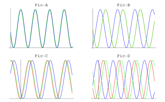
Figure 1: The four graphs represent four small-time-spans, red curve represents the $P^{T}$, green the $P_{I}$, and blue the $P$. We do not mark the ticks because the time span is so small that the Mathematica tool can not even mark them clearly,yet this does not imped us to see the differences among the three curves of the four graphs above. The Pic-A shows while t is around $10^{-7}$s, $P^{T}$, $P_{I}$ and $P$ coincide with each other. Pic-B shows while t is around $1$s, $P^{T}$ and $P_{I}$ still coincide with each other, but $P$ begins to deviate. Pic-C shows when $t$ is around $6s$, $P_{I}$ begins to stray away from $P^{T}$, while $P$ also deviates from the former two. Pic-D shows when t is around $27.7$s, obvious deviations between $P^{T}$ and $P_{I}$ occur, and $P$ still shows irregular deviation.

FIG.1 tells us that when time $t$ is very small, say $10^{-7}$s, the transition probability of traditional way and new way both coincide with the exact solution. However, when time evolves to a relatively large value, traditional result show irregular deviation from the exact one, while new result still matches well with it. Of course, new result also will deviate from the exact one when time $t$ is large enough. Therefore we can say that, when the magnitude of magnetic field is given, traditional result is useful only when time $t$ is small enough, but new one will be exact in a large time-span. As a result, we clearly see the advantage of new way of perturbation theory. Next, we will compare the three curves when time “$t$” is set and magnetic field is changing.

IV.2 COMPARISON OF TRANSITION PROBABILITY AS MAGNETIC FIELD CHANGES

At the given time we choose the time $t=1$s. We also choose four small magnetic field spans, and FIG.2 represents the comparison of three curves: $P^{T}$, $P_{I}$ and $P$. Here we write down the expression of them:

$$\begin{array}[]{r@{\quad=\quad}l}P^{T}&\dfrac{\sin^{2}(\sqrt{1.991244499780254521326\times 10^{19}+7.751567612132237407735\times 10^{21}\times B^{2}})}{1+389.2825623868\times B^{2}}\\[8.0pt] P_{I}&\sin^{2}(4.462336271259\times 10^{9}+8.685548489539\times 10^{11}\times{B^{2}}-8.452831429358\times 10^{13}\times{B^{4}})\\[8.0pt] P&\sin^{2}(4.462336271259\times 10^{9})\end{array}$$ (45)

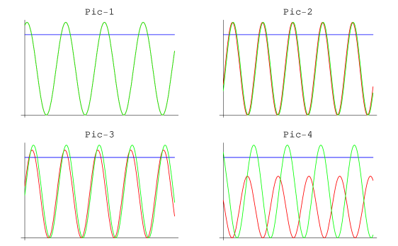
Figure 2: In the graph above, the red curve represents $P^{T}$, green the $P_{I}$ and blue the $P$. Curve $P$ is a straight line which is independent to $B$. Pic-1 shows when $B$ is around $10^{-4}$T, $P^{T}$ and $P_{I}$ coincide with each other. Pic-2 shows when $B$ is around $1.29\times 10^{-3}$T, nuance between $P^{T}$ and $P_{I}$ appears. Pic-3 shows when $B$ is around $1.21\times 10^{-2}$T, there is obvious distinction between them. Pic-4 shows when $B$ is around $0.036$T, huge difference occurs, and even their oscillation amplitudes are different.

In this part, we again see the differences between traditional result and new one. In fact, in this case the phase factor of traditional transition probability has nothing to do with magnetic field, which results in the straight line in FIG.2. However, as we can see from the exact solution, the transition probability oscillate intensively with the change of $B$, and this reveals the defect of traditional way. Yet, new way in wang1 provide us with a relatively satisfying expression, which also vibrates with magnetic field “$B$”. This new expression matches well with exact solution when “$B$” varies in a certain range. Yet, we should notice that there is also some flaw in the new result, which can be seen from the Pic-4 in FIG.2. Such flaw results from the difference of denominators between Eqs. (8) and (36), which will influence their vibration amplitudes.

V Discussion and Conclusion

Now we will come to a conclusion. In Ref. wang1 , the author gives a improved form of perturbed solution of dynamics, it is interesting to study its influences on some physics results. As we can see, the phase factors correlating to dynamical behavior in the expression of state vector are changed, and the variations absorb the partial contributions from higher order approximations. This leads us to consider the change of transition probability. Since abstract discussion of the transition probability is both hard and has no common meaning, we should find concrete cases to discuss.

Main work we do in this paper is to calculate the improved transition probability for a Hydrogen atom in a constant magnetic field. In fact, this example we choose is appropriate, because we need to choose one which can be given the exact solution so that we can compare it with the result of traditional and Wang’s scheme of perturbation theory. The comparison we give in Sec. IV successfully indicate that Wang’s scheme does show its advantages beyond traditional one. Perhaps someone would argue that this example is too simple to be meaningful enough, however, we should note that such simple case do suggest that some expressions such as transition probability in other cases might need amended, or at least need perfected. Maybe such amendment does not have huge influence in some systems, but to extend this assertion to all problems is both too early and too cursory.

In fact, Ref. wang1 uses several skillful ways to include the high-order approximation in the expression of low-order one, and this procedure results in a tidy expression of perturbed solution of dynamics. It is a physical reason why Wang’s scheme can improve the existed some conclusions. Finally, since we also see the flaw shown in Pic-4 of Fig.2, perhaps there will still be further amendment to it in the future.

References

• (1) An Min Wang, “Quantum mechanics in general quantum systems (I) and (II): exact solution and perturbation theory”; quant-ph/0602055 v7
• (2) Krzysztof Pachucki,Physical Review A, vol.54, number 3, 1996
• (3) M.Nio, T.Kinoshita, Physical Review D, vol.55, No.11, 1997
• (4) W.Liu, M.G.Boshier,S.Dhawan, Physics Review Letters,Vol.82, No.4,1999
• (5) Peter J. Mohr, Barry N. Taylor, Rev. Mod. Phys, vol77, pp1-107(2005)
• (6) E. R. Cohen and B. N. Taylor, T. Phys. Chem. Ref. Data 2, 663(1973)