Precision measurement with an optical Josephson junction

Abstract

We study a new type of Josephson device, the so-called “optical Josephson junction” as proposed in Phys. Rev. Lett. 95, 170402 (2005). Two condensates are optically coupled through a waveguide by a pair of Bragg beams. This optical Josephson junction is analogous to the usual Josephson junction of two condensates weakly coupled via tunneling. We discuss the use of this optical Josephson junction, for making precision measurements.

I Introduction

Atom optics has obtained an unprecedented development since the advent of Bose-Einstein condensates (BEC’s) of dilute alkali atomic gases Bradley . For instance, the applications of atom optics have been realized such as atom laser, solition generation Rolston and matter wave interferometry Shin0 . Besides, many new techniques of manipulating the cold atoms have been devised such as Bragg scattering Kozuma and magnetic waveguide Leanhardt , etc. These sophisticated techniques may lead to reaching the goal in higher precision measurement Dunningham and applications in quantum information processing Nielsen .

Recently, Saba et. al Saba and Shin et. al Shin have demonstrated that the Josephson effect by using the technique of atom optics, Bragg scattering. Two beams of atoms are optically extracted from two separate trapped Bose-Einstein condensates (BEC’s) using Bragg scattering Kozuma . Then, these two beams of atoms overlap and interfere with each other and the measurement process creates a relative phase between the two BEC’s. They showed that the Josephson coupling of these two spatially separate systems can be made through an intermediate coupling system. It is quite different to the conventional Josephson devices, such as superconducting systems Anderson , and Bose-Einstein condensates Cataliotti , in which the two quantum systems are spatially connected to each other and the wavefunction of them have small overlap.

In this paper, we investigate that the two trapped condensates are connected by outcoupling a small fraction of condensates via the Bragg scattering Kozuma and those outcoupling atoms are transported through a magnetic waveguide Leanhardt to replenish the trapped condensates Shin . We show that this system is equivalent to the usual Hamiltonian describing the Josephson effect of BEC’s trapped in a double-well potential. The strength of the Josephson coupling can be explicitly controlled by varying the outcoupling rate of atoms using the Bragg beams whereas the coupling phase between these two condensates can be tuned by adjusting the phase shifts of the outcoupled atoms Shin . Moreover, the spontaneous scattering due to the Bragg beams is negligible by virtue of the large detuning of the pulses. This “optical Josephson junction” could be used, for example, to implement the precision scheme proposed by Dunningham and Burnett Dunningham in which they consider the precision measurement using an entangled BEC’s trapped in a double-well potential.

We now study the implementation of the precision measurement scheme being suggested by Dunningham et al. Dunningham , which can measure the nonlinear interaction strength and gravity, using this “optical Josephson junction”. According to this proposal, the measurement of phase can be done by appropriately turning on and off the Josephson coupling. Then, the final phase information is encoded in the number fluctuation that can be detected from the collapse and revival of the relative phase between the condensates. This scheme provides a simple way to measure phase with Heisenberg limited accuracy, i.e., the phase uncertainty scales as $1/N$, where $N$ is the number of atoms.

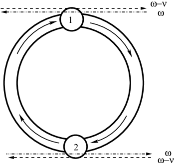
Figure 1: The schematic of the optical coupling of two trapped condensates 1 and 2, and the outcoupling atoms are transferred via a waveguide in the ring form. The pair of Bragg beams with frequencies $\omega$ and $\omega-\nu$ are denoted by dash-dot line and dash line respectively.

The paper is organized as follows: In Sec. II, we introduce the model of this “optical Josephson junction”. In Sec. III, we derive an effective Hamiltonian under the two-mode approximation of two trapped BEC’s. In Sec. IV, we study the implementation of Dunningham et al. scheme in this system. We briefly review the mechanism of the Bragg scattering in appendix A.

II Basic model

We consider two trapped condensates connected to a 1D ring-form waveguide using the $M$-th order Bragg scattering Saba ; Shin as shown in Fig 1. In fact, this Bragg scattering is a $2M$-th order multi-photon Raman process Kozuma ; Berman . The stimulated emission and stimulated absorption are made by using the two Bragg beams being acted as a pump and probe field with counter-propagation and slightly frequency difference, i.e., $\omega=$ and $\omega-\nu$. The wavelength and wave number of the Bragg beam with frequency $\omega$ are $\lambda$ and $k=2\pi/\lambda$ respectively.

This pair of Bragg beams give out a certain amount of momentum to the two trapped BEC’s $1$ and $2$ respectively. Then, a small amount of BEC’s are outcoupled from these two trapped BEC’s with definite momenta ${\hbar}k_{1}$ and ${\hbar}k_{2}$ at the $M$-th order Raman process. Without loss of generality, we assume the two momenta $k_{1}$ and $k_{2}$ with the equal magnitude but opposite sign, for $\hbar^{2}k^{2}_{1,2}/2m=M\hbar\nu$ and $m$ is the mass of an atom. These outcoupling condensates are then transported via the waveguide to the other trapped BEC. This conservation of total number of particles may enable us to overcome the limitation of the coupling time in the experiments Saba ; Shin in which the atoms were linearly coupled out and not transferred back to the system Shin . But now the coupling process can be continued if the number of atoms are conserved in the system.

We discuss the Hamiltonian of this system and derive an effective two-state Hamiltonian to describe the Josephson effect. The Hamiltonian of the total system has the form

$$H = H_{0}+H_{\rm ring}+H_{\rm couple},$$ (1)

where $H_{0}$, $H_{\rm ring}$ and $H_{\rm couple}$ are the Hamiltonians of; BEC’s 1 and 2, the outcoupled atoms in the 1D ring, and the coupling between the trapped atoms and the ring respectively. The Hamiltonian for the trapped atoms has the form and can be expressed in terms of the arc length, $s=r\phi$ for $r$ is the radius of the ring and $\phi$ is the polar angle of the ring,

$$H_{0} = \sum^{2}_{j=1}\oint{ds}\Bigg{\{}\Psi^{{\dagger}}_{j}(s)\Bigg{[}-\frac{\hbar^{2}}{2m}\frac{\partial^{2}}{\partial{s^{2}}}+V_{j}(s)\Bigg{]}\Psi_{j}(s)$$ (2)

$$+\frac{U_{0}}{2}\Psi^{\dagger}_{j}(s)\Psi^{\dagger}_{j}(s)\Psi_{j}(s)\Psi_{j}(s)\Bigg{\}},$$

where $\Psi_{j}(s)$ and $V_{j}(s)$ are the field operator and trapping potential respectively for condensate $j$, $U_{0}$ is the interaction strength and $j=1,2$.

We consider that the two condensates are held in two different traps that are sufficiently deep, and hence the single-mode approximation can be applied Milburn . This allows us to describe the trapped condensates as the local ground state of the trap. The field operator $\Psi_{j}(s)$ can then be approximated by ${c_{j}}\psi_{j}(s)$, where $c_{j}$ and $\psi_{j}(s)$ are the annihilation operators and the mode function of the potential of the $j$-th trap and $j=1,2$. If we take the system to be symmetric so that $\Psi_{1}(s)$ has the same form as $\Psi_{2}(s)$, the Hamiltonian $H_{0}$ can be written as

$$H_{0} = E_{0}(c^{\dagger}_{1}c_{1}+c^{\dagger}_{2}c_{2})+\frac{\hbar\kappa}{2}[(c^{\dagger}_{1}c_{1})^{2}+(c^{\dagger}_{2}c_{2})^{2}],$$ (3)

where

$$E_{0} = {\oint}ds\psi^{*}_{j}(s)\Bigg{[}-\frac{\hbar^{2}}{2m}\frac{\partial^{2}}{\partial{s^{2}}}+V_{j}(s)\Bigg{]}\psi_{j}(s),$$ (4)

is the eigenenergy of the two modes and

$$\kappa = U_{0}\oint{ds}|\psi^{*}_{j}(s)\psi_{j}(s)|^{2},$$ (5)

is the self-interaction strength.

The free condensates can be outcoupled from the trapped condensate using the Bragg scattering Kozuma . We briefly review its mechanism in the appendix A. The nearly perfect efficiency of the first order Bragg resonance has been observed experimentally Kozuma . However, the efficiency of the high order Bragg scattering is decreased significantly Kozuma . The Hamiltonian representing the effective coupling between the trapped atoms and the free condensate is written, thus,

$$H_{\rm couple}=\gamma\oint{ds}[\Psi^{\dagger}_{f}(s)\Psi_{1}(s)+{e^{-i\pi\delta{k}r}}\Psi^{\dagger}_{f}(s)\Psi_{2}(s)]+{\rm H.c.},$$ (6)

where ${\gamma}$ is the outcoupling amplitude between two trapped BEC’s and free outcoupling condensates Choi , $\delta{k}=k_{1}+k_{2}-4k$ Shin respectively. Here, we can consider the coupling between the trapped condensates and the free condensates with momenta $k_{1,2}$. Moreover, we consider the replenishment process in which the free condensates are deaccelerated by the Bragg beams and merge into the trapped condensates Chikkatur . We assume that the excitation in this replenishing process is negligible. On the other hand, the relative phase shift $\pi\delta{k}r$ is generated during the flight between the two condensates. The phase shift $\delta{k}$ directly depends on the Bragg beams and the momenta $k_{1,2}$ which can be adjusted in the experiment Shin .

The Hamiltonian of the 1D ring has the corresponding form:

$$H_{\rm ring} = \oint{ds}\Bigg{[}\Psi^{{\dagger}}_{f}(s)\Bigg{(}-\frac{\hbar^{2}}{2m}\frac{\partial^{2}}{\partial{s^{2}}}\Bigg{)}\Psi_{f}(s)$$ (7)

$$+\frac{U_{0}}{2}\Psi^{\dagger}_{f}(s)\Psi^{\dagger}_{f}(s)\Psi_{f}(s)\Psi_{f}(s)\Bigg{]},$$

where $\Psi_{f}(s)$ is the field operator of the condensate in this ring-form waveguide transported by a waveguide. We approximate these unconfined in the angular direction, but confined radially and weakly interacting condensate as the freely propagating non-interacting condensates. We can justify this approximation by considering the magnitude of the kinetic energy and the strength of the nonlinear interaction. The kinetic energy $\hbar\omega_{k_{j}}$ of the outcoupled condensates by the Bragg beams is with $\omega_{k_{j}}{\sim}10^{2}$ kHz Shin whereas the nonlinear interaction of this nearly free condensates $n_{0}U_{0}/\hbar$ is about ${1}$ kHz Leggett . Here $n_{0}$ is density of the outcoupled condensate which must satisfy $n_{0}a_{s}{\ll}1$ and $a_{s}$ is the scattering length of the atom. From the above estimation, we can argue that this weakly interacting outcoupled condensates as free condensates.

The condensates in the ring are composed of two free condensates outcoupled from the two trapped condensates as

$$\Psi_{f}(s) = {(2\pi{r})}^{-1/2}(e^{ik_{1}s}g_{k_{1}}+e^{ik_{2}s}g_{k_{2}}),$$ (8)

where $2\pi{r}$ is the circumference of the loop, $k_{1,2}$ should satisfy the boundary condition $k_{1,2}r={\alpha}\hbar$ and $\alpha$ is an integer. Then, the Hamiltonian of the ring can be written as

$$H_{\rm ring} = \sum^{2}_{j=1}\hbar\omega_{k_{j}}g^{\dagger}_{k_{j}}g_{k_{j}},$$ (9)

where $\omega_{k_{i}}={\hbar}k^{2}_{i}/2m$.

III Effective Hamiltonian

We now derive an effective Hamiltonian to describe the Josephson effect between two trapped BEC’s. The free propagating condensates act as immediate states to couple the two trapped condensates. The coupling Hamiltonian is given by

$$H_{\rm couple}=\hbar\sum^{2}_{j=1}\gamma^{\prime}(k_{j})(c^{\dagger}_{1}+e^{i\theta}c^{\dagger}_{2})g_{k_{j}}+{\rm H.c.},$$ (10)

where $\gamma^{\prime}(k_{j})=\gamma(2\pi{r})^{-1/2}\oint{ds}e^{-i{k_{j}}s}\psi_{j}(s)$, $j=1,2$ and $\theta=\pi\delta{k}r$. We assume that the two coupling strengths $\gamma^{\prime}(k_{j})$ are similar by letting $\oint{ds}e^{-ik_{1}s}\psi_{1}(s)\approx\oint{ds}e^{-ik_{2}s}\psi_{2}(s)$. The Heisenberg equation of motion of $g_{k_{j}}$ is

$$i\dot{g}_{k_{j}} = \omega_{k_{j}}g_{k_{j}}+\gamma^{\prime}(k_{j})(c_{1}+e^{-i\theta}c_{2}).$$ (11)

We use the adiabatic approximation, i.e., $\dot{g}_{k_{j}}{\approx}0$ as the condition $\omega_{k_{j}}{\gg}|\gamma^{\prime}(k_{j})|$ is satisfied:

$$g_{k_{j}} \approx -\frac{\gamma^{\prime}(k_{j})}{\omega_{k_{j}}}(c_{1}+e^{-i\theta}c_{2}).$$ (12)

We can see that it is true if we can assure that $\gamma$ is much less than $\omega_{k_{1,2}}$. Physically speaking, the validity of this adiabatic approximation assumes that the transition time between these intermediate states and the two trapped states is short enough. Moreover, it is noted that the whole $2M$-th order Raman process requires a finite time duration with the interaction of laser to be completed. This time duration must be short compared to the time of the Josephson coupling.

The resulting effective two-state Hamiltonian can thus be written as

$$H_{\rm eff} = \Bigg{(}E_{0}-\frac{{\hbar}g}{2}\Bigg{)}(c^{\dagger}_{1}c_{1}+c^{\dagger}_{2}c_{2})+\frac{\hbar\kappa}{2}[(c^{\dagger}_{1}c_{1})^{2}+(c^{\dagger}_{2}c_{2})^{2}]$$ (13)

$$-\frac{{\hbar}g}{2}\Big{(}e^{-i\theta}c^{\dagger}_{1}c_{2}+e^{i\theta}c^{\dagger}_{2}c_{1}\Big{)},$$

where $g=2\sum^{2}_{j=1}{\gamma^{\prime}}^{2}(k_{j})/\omega_{k_{j}}$. It is noteworthy that this effective two-mode Hamiltonian is akin to the Josephson Hamiltonian of the external Milburn and the internal Sorensen BEC systems. This optical Josephson coupling can then yield the Josephson effect of two condensates. Likewise, this Josephson coupling can be controlled by the strength of the Bragg beam to vary $g$ whereas the phase of Josephson coupling can be adjusted by the phase shift $\theta$ that can be done by changing $k$ and the arc length between the BEC’s. Indeed, this feature is very useful to the application of this Josephson junction.

It is convenient to write the effective Hamiltonian in terms of the angular momentum operators as

$$J_{x} = \frac{1}{2}(c^{\dagger}_{1}c_{2}+c^{\dagger}_{2}c_{1}),$$ (14)

$$J_{y} = \frac{1}{2i}(c^{\dagger}_{1}c_{2}-c^{\dagger}_{2}c_{1}),$$ (15)

$$J_{z} = \frac{1}{2}(c^{\dagger}_{2}c_{2}-c^{\dagger}_{1}c_{1}),$$ (16)

where the total atom numbers $N=c^{\dagger}_{2}c_{2}+c^{\dagger}_{1}c_{1}$ is conserved. Then, the Hamiltonian is written as

$$H_{\rm eff} = \hbar\kappa{J^{2}_{z}}+{\hbar}g(\cos\theta{J_{x}}+\sin\theta{J_{y}})+C,$$ (17)

where $C=(E_{0}-{\hbar}g/2)N+\kappa{N^{2}}/4$. This constant $C$ does not affect the quantum dynamics of the system. Therefore, we will ignore it in the subsequent discussion.

IV Implementation of precision measurement

In this section, we discuss the implementation of precision measurement on the optical Josephson junction. Dunningham and Burnett proposed a precision measurement scheme using a number-squeezed BEC trapped in a double-well potential Dunningham . This scheme requires the active control of the Josephson coupling. The phase information can be finally obtained by measuring the number fluctuations which can be detected via the visibility of the interference fringes of the two condensates. However, there are some limitations of the BEC double-well system with respect to the dynamical control of the Josephson coupling. The Josephson coupling strength exponentially depends on the height of potential barrier between the two wells. The potential barrier has to be tuned very accurately in order to vary the coupling.

Besides, when the Josephson coupling is large, there needs to be a large spatial overlap between the two localized wave functions in two wells. In this case, the usual two-mode approximation is no longer valid. This problem can now be avoided in the optical Josephson junction system due to the large separation between the two trapped condensates. Since the optical Josephson junction is a well-controlled system, it is a promising model to implement this scheme.

We proceed to describe how to realize the protocol of the scheme proposed by Dunningham et al.. If we choose the phase shift $\theta=\pi$, the effective Hamiltonian has the form,

$$H_{\rm eff} = \hbar\kappa{J^{2}_{z}}+{\hbar}g{J_{x}}.$$ (18)

We first prepare the initial state as a number-squeezed state $|N/2\rangle_{1}|N/2\rangle_{2}$ which contains a definite number of atoms trapped in two wells respectively. This can be prepared by adiabatically switching off the Josephson coupling strength so that the condensates are isolated in two different traps in the Fock regime, i.e., $g\ll{\kappa{N}}$ Leggett .

We can use this system to measure a relative phase between the condensates as follows. A large Josephson coupling is turned on rapidly with the strength $g\gg{\kappa{N}}$ by using Bragg pulses with $g=g^{*}$. It is convenient to write the state in the new eigenbasis, i.e., the symmetric mode $\alpha=(c_{1}+c_{2})/\sqrt{2}$ and antisymmetric mode $\beta=(c_{1}-c_{2})/\sqrt{2}$ with respect to two traps. The quantum state is in this new basis, has the form Dunningham

$$|\Psi\rangle = \sum^{N/2}_{m=0}(-1)^{m}C_{m}|2m\rangle_{\alpha}|N-2m\rangle_{\beta},$$ (19)

where $C_{m}=\sqrt{(2m)!(N-2m)!}/2^{N/2}m!(N/2-m)!$. It is worth noting that this superposition of states is robust against the particle loss Dunningham2 . In this regime, there is a small energy difference, $g^{*}$, between the symmetric and antisymmetric modes, different phases result for the terms in the superposition. Then, the system is held for a certain time $t=t^{*}$ to allow the natural evolution of the system.

Next, the Josephson coupling is suddenly switched off fast enough with respect to coupling between wells, but slow with respect to energy level spacing in each well. Thus, the state is conveniently expressed in terms of the number basis in each well. The quantum state becomes Dunningham

$$|\Psi\rangle = \frac{1}{2^{N/2}{(N/2)}!}\sum^{N}_{n=0}(-1)^{n}D_{n}|n\rangle_{1}|N-n\rangle_{2},$$ (20)

where

$$D_{n}=\sum^{k/2}_{p={\rm max}\{0,n-{N}/{2}\}}\left(\begin{array}[]{c}{N}/{2}\\ p^{*}\end{array}\right)\left(\begin{array}[]{c}p^{*}\\ p\end{array}\right)\sqrt{n!(N-n)!}(i\sin\phi)^{p^{*}}(2\cos\phi)^{n-2p}$$ (25)

for $p^{*}=N/2-n+2p$ and $\phi={\hbar}g^{*}{t^{*}}$. This completes the measurement of the phase $\phi$ which is recorded in the quantum state now. The information of this phase $\phi$ can be obtained from the number uncertainty ${\Delta}n$, where $n=c^{\dagger}_{1}c_{1}=N-c^{\dagger}_{2}c_{2}$ is the number of atoms in the trap 1 (or 2). From Eq. (20), the number uncertainty can be calculated as Dunningham

$$\Delta{n} = \frac{N}{2\sqrt{2}}\sin\phi.$$ (26)

This number uncertainty is of order $N$. According to the number-phase uncertainty relation $\Delta{n}\Delta{\phi}\sim{1}$, we can see that the uncertainty of the phase $\phi$, for the minimum uncertainty state, is of order $N^{-1}$, i.e., Heisenberg limited.

This number variance can be experimentally determined from the interference pattern. Bragg scattering provides a non-destructive method to determine the relative phase. A small fraction of condensates are coupled out horizontally from these two condensates and allowed to interfere with each other. The relative phase between the two trapped condensates can be determined from the interference patten of these two outcoupled condensates Wright ; Dunningham3 . The interference pattern of the fringes between the two outcoupled condensates Sinatra , $I=\int{dx}[\Psi^{\dagger}_{f1}(x)\Psi_{f2}(x)+\Psi^{\dagger}_{f2}(x)\Psi_{f1}(x)]$, is directly proportional to the interference terms of two trapped condensates, where $\Psi_{f1}$ and $\Psi_{f2}$ are the field operator of two outcoupled condensates from the $j$-th trap, and $x$ is coordinate in the horizontal direction. Following the similar treatment to the previous section and taking $\theta=\pi$, the intensity of the interference fringes, $I$, of these two outcoupled condensates can be obtained as Sinatra

$$I=\frac{\gamma^{\prime}(k_{1})\gamma^{\prime}(k_{2})}{\omega_{k1}\omega_{k_{2}}}\langle\psi(\tau)|{c}^{\dagger}_{1}c_{2}+{c}^{\dagger}_{2}c_{1}|\psi(\tau)\rangle,$$ (27)

where $\tau$ is the time of holding the system with the nonlinear interaction of the atoms. This state vector is given by

$$|\psi(\tau)\rangle=\frac{1}{2^{N/2}{(N/2)}!}\sum^{N}_{n=0}(-1)^{n}e^{-i{\hbar\kappa}[n^{2}+(N-n)^{2}]\tau/2}D_{n}|n\rangle_{1}|N-n\rangle_{2}.$$ (28)

Thus, the intensity, $I$, is proportional to

$$I(\tau) \propto \sum_{n}D^{*}_{n+1}D_{n}\sqrt{(n+1)(N-n)}e^{i\hbar\kappa(2n+1-N){\tau}}$$ (29)

$$+D^{*}_{n-1}D_{n}\sqrt{n(N-n+1)}e^{i\hbar\kappa(N-2n+1){\tau}}.$$

The collapse times $t_{\rm coll}$ can be estimated by considering the particle numbers in the range, $n=N/2\pm\Delta{n}/2$. Hence, the collapse times of the relative phase $t_{\rm coll}$ is about $\pi/2\hbar\kappa\Delta{n}$ Wright ; Dunningham3 . This collapse time can be determined by holding the system with the nonlinear interaction as a function of time $\tau$ and measure the corresponding intensity $I$ with different $\tau$’s. Therefore, we can determine the number fluctuation and hence the required phase information.

From an experimental point of view, the collapse time is very short and so the damping and decoherence effects may be minimized. Hence, the number variance may be able to be measured accurately by this method. Although the revival time can reveal the phase information, it takes a much longer time to observe. Bear in mind that the measurement of collapse and revival time of a Bose-Einstein condensate has been demonstrated in the experiment Greiner .

V Discussion

It is noted that the low efficiency of the higher order Bragg scattering may limit the effective coupling of the two coupled BEC’s. Nevertheless, we can still justify the validity of this optical based Josephson junction as discussed above. On the other hand, it is very interesting to compare this optical based Josephson junction to the solid-state counterpart.

In summary, we theoretically study the microscopic model of the “optical Josephson junction” and derive the effective Hamiltonian of this device. We have discussed how this system can be used to implement Hesienberg limited precision measurement. This measurement can be made by detecting the collapse time non-destructively.

Appendix A Bragg scattering

In this appendix, the basic mechanism of the condensates using the Bragg scattering is briefly reviewed. The pump-probe mechanism has been discussed in detail in the reference Berman . The pump and probe fields impart a momentum $2k$ to the ground state of the condensates each time by coupling to the excited state with a large detuning $\Delta=\tilde{\omega}-\omega$ between the two-level atoms with the energy difference $\hbar\tilde{\omega}$ and the laser field. To elucidate this process, we study the first order Bragg resonance case by considering a time-independent Hamiltonian in the interaction picture and assume the zero ground state energy for $g_{0}$ which is given by

$$H_{\rm 1st} = \hbar{\Delta}_{1}{e}^{\dagger}_{k}e_{k}+\hbar({\Delta}_{1}-{\Delta}_{2})g^{\dagger}_{2k}g_{2k}+\hbar\Omega(g^{\dagger}_{0}e_{k}+e^{\dagger}_{k}g_{0})$$ (30)

$$+\hbar\Omega^{\prime}(g^{\dagger}_{2k}e_{k}+e_{k}g^{\dagger}_{2k}),$$

where $e_{nk}$ and $g_{nk}$ are the annihilation operators for the excited and ground states with the momentum $nk$, $\Omega$ and $\Omega^{\prime}$ are the coupling strength of the pump field and the probe field of this pair of Bragg beams; and ${{\Delta}}_{1}=\Delta+\omega_{k}$ and ${\Delta}_{2}=\Delta+\omega_{k}-\omega_{2k}+\nu$ are the detuning between the ground and the excited states with the different momenta and the Bragg beams, for $\omega_{nk}=\hbar(nk)^{2}/2m$.

The equations of motion for the different momentum states are given by:

$$i\dot{g}_{0} = \Omega{e}_{k},$$ (31)

$$i\dot{e}_{k} = {\Delta}_{1}e_{k}+\Omega{g}_{0}+\Omega^{\prime}g_{2k},$$ (32)

$$i\dot{g}_{2k} = ({\Delta}_{1}-{\Delta}_{2})g_{2k}+\Omega^{\prime}e_{2k}.$$ (33)

At the Bragg resonance, the detuning ${\Delta}_{1}-{\Delta}_{2}=4\omega_{k}-\nu$ equals zero at $\nu=4\omega_{k}$. The excited state $e_{k}$ can be adiabatically eliminated as ${\Delta}_{1}\gg\Omega$,$\Omega^{\prime}$, i.e.,

$$e_{k} = -\frac{1}{{\Delta}_{1}}(\Omega{g}_{0}+\Omega^{\prime}g_{2k}).$$ (34)

Therefore, the equations of motion for these two ground states with different moment have the form:

$$i\dot{g}_{0} = -\frac{1}{{\Delta}_{1}}(\Omega^{2}g_{0}+\Omega\Omega^{\prime}g_{2k}),$$ (35)

$$i\dot{g}_{2k} = -\frac{1}{{\Delta}_{1}}(\Omega\Omega^{\prime}g_{0}+\Omega^{\prime 2}g_{2k}).$$ (36)

Clearly, we can see that these two momentum states are effectively coupled with each other at the first order Bragg resonance.

In general, we can consider the $M$-th order Bragg scattering which is a $2M$-th multi-photon Raman process. Within this process, the different momentum modes are virtually excited but they can be adiabatically eliminated because of energy conservation being unfavourable. It is legitimate to consider the effective coupling between the trapped condensates and the free momentum states $\hbar{\omega_{k_{1,2}}}=M{\nu}$ at the Bragg resonance only in which the energy is conserved. The explicit form of the effective coupling between the trapped and free states, ${\gamma}$, has been found as Berman :

$${\gamma} = \Bigg{|}\frac{(\Omega\Omega^{\prime}/{\Delta})^{M}}{[(M-1)!]^{2}\omega^{M-1}_{2k}}\Bigg{|}.$$ (37)

The detailed analysis can be referred to the reference Berman .

References

- (1) C. C. Bradley et al., Phys. Rev. Lett. 75, 1687 (1995); K. B. Davis et al., ibid. 75, 3969 (1995); M. H. Anderson et al., Science 269, 198 (1995).
- (2) S. L. Rolston and W. D. Phillips, Nature 416, 219-224 (2002).
- (3) Y. Shin et al., Phys. Rev. Lett. 92, 050405 (2004).
- (4) M. Kozuma et al., Phys. Rev. Lett., 82, 871 (1999); J. Stenger et al., ibid. 82, 4569 (1999).
- (5) A. E. Leanhardt et al., Phys. Rev. Lett., 89, 040401 (2002).
- (6) J. A. Dunningham and K. Burnett, Phys. Rev. A 70, 033601 (2004).
- (7) M. A. Nielsen and I. L. Chuang, Quantum Computation and Quantum Information (Cambridge University Press, Cambridge, 2000).
- (8) M. Saba et al., Science 307, 1945 (2005).
- (9) Y. Shin et al., Phys. Rev. Lett. 95, 170402 (2005).
- (10) P. W. Anderson and J. W. Rowell, Phys. Rev. Lett. 10, 230 (1963).
- (11) F. S. Cataliotti et al., Nature 388, 449 (1997); M. Albiez et al., Phys. Rev. Lett. 95, 010402 (2005).
- (12) P. R. Berman and, B. Bian, Phys. Rev. A 55, 4382 (1997).
- (13) S. Choi, Y. Japha and K. Burnett, Phys. Rev. A 61, 063606 (2000).
- (14) A. P. Chikkatur et al., Science, 296, 2193 (2002).
- (15) G. J. Milburn, J. Corney, E. M. Wright and D. F. Walls, Phys. Rev. A 55, 4318 (1997).
- (16) A. Sorensen, L. M. Duan, J. I. Cirac and P. Zoller, Nature 409, 63 (2001); C. K. Law, H. T. Ng and P. T. Leung, Phys. Rev. A 63, 055601 (2001).
- (17) A. J. Leggett, Rev. Mod. Phys. 73, 307 (2001).
- (18) J. A. Dunningham, K. Burnett and S. M. Barnett, Phys. Rev. Lett. 89, 150401 (2002).
- (19) E. M. Wright, D. F. Walls and J. C. Garrison, Phys. Rev. Lett. 77, 2158 (1996).
- (20) J. A. Dunningham, M. J. Collett and D. F. Walls, Phys. Lett. A 245, 49 (1998).
- (21) A. Sinatra and Y. Castin, Eur. Phys. J. D 4, 247 (1998).
- (22) M. Greiner, O. Mandel, T. W. Hänsch and I. Bloch, Nature 419, 51 (2002).