Continuous Variable Quantum Cryptography
using Two-Way Quantum Communication

Quantum cryptography has been recently extended to continuous variable systems, e.g., the bosonic modes of the electromagnetic field. In particular, several cryptographic protocols have been proposed and experimentally implemented using bosonic modes with Gaussian statistics. Such protocols have shown the possibility of reaching very high secret key rates, even in the presence of strong losses in the quantum communication channel. Despite this robustness to loss, their security can be affected by more general attacks where extra Gaussian noise is introduced by the eavesdropper. In this general scenario we show a “hardware solution” for enhancing the security thresholds of these protocols. This is possible by extending them to a two-way quantum communication where subsequent uses of the quantum channel are suitably combined. In the resulting two-way schemes, one of the honest parties assists the secret encoding of the other with the chance of a non-trivial superadditive enhancement of the security thresholds. Such results enable the extension of quantum cryptography to more complex quantum communications.

In recent years, quantum information has entered the domain of continuous variable (CV) systems, i.e., quantum systems described by an infinite dimensional Hilbert space CVbook ; BraReview . So far, the most studied CV systems are the bosonic modes, such as the optical modes of the electromagnetic field. In particular, the most important bosonic states are the ones with Gaussian statistics, thanks to their experimental accessibility and the relative simplicity of their mathematical description EisertGauss ; GaussianStates . Accordingly, quantum key distribution (QKD) has been extended to this new framework Hillery ; Ralph1 ; Ralph2 ; Reid ; Preskill ; Cerf0 ; Homo ; Homo2 ; Cerf ; Cerf2 ; Hetero ; Hetero2 ; Silber ; Hirano1 ; Hirano2 ; Hirano3 ; Lutk and Gaussian cryptographic protocols using coherent states have been shown to exploit fully the potentialities of quantum optics Homo2 ; Hetero2 . These coherent-state protocols are robust with respect to the noise of the quantum channel, as long as such noise can be ascribed to pure losses Homo2 ; Hetero2 . By contrast, their security is strongly affected when channel losses are used to introduce a thermal environment, which is assumed to be controlled by a malicious eavesdropper Homo2 ; Estimators . In this Gaussian eavesdropping scenario, we present a method to enhance the security thresholds of the basic coherent-state protocols. This is achieved by extending them to two-way quantum communication protocols, where one of the honest parties (Bob) uses its quantum resources to assist the secret encoding of the other party (Alice). In particular, the enhancement of security is proven to be effective since the security thresholds are superadditive with respect to the double use of the quantum channel. Such a result is achieved when the Gaussian attack corresponds to a memoryless Gaussian channel. More generally, we also consider Gaussian channels with memory, therefore creating classical and/or quantum correlations between the paths of the two-way quantum communication. In order to overcome this kind of eavesdropping strategy, the two-way protocols must be modified into suitable hybrid protocols, which represent their safe formulation against every kind of collective Gaussian attack.

I One-way protocols

In basic coherent-state protocols Homo ; Hetero , Alice prepares a coherent state $\left|\alpha\right\rangle$ whose amplitude $\alpha=(Q_{A}+iP_{A})/2$ is stochastically modulated by a pair of independent Gaussian variables $\{Q_{A},P_{A}\}$, with zero mean and variance $V-1$. This variance determines the portion of phase space which is available to Alice’s classical encoding $\{Q_{A},P_{A}\}$ and, therefore, quantifies the amount of energy which Alice can use in the process. This energy is usually assumed to be very large $V\gg 1$ (large modulation limit) in order to reach the optimal and asymptotic performances provided by the infinite dimensional Hilbert space. The modulated coherent state is then sent to Bob through a quantum channel, whose noise is assumed ascribable to the malicious action of a potential eavesdropper (Eve). In a homodyne ($Hom$) protocol Homo , Bob detects the state via a single quadrature measurement (i.e., by a homodyne detection). More exactly, Bob randomly measures the quadrature $\hat{Q}$ or $\hat{P}$, getting a real outcome $X_{B}=Q_{B}$ (or $P_{B}$) which is correlated to the encoded signal $X_{A}=Q_{A}$ (or $P_{A}$). In a heterodyne ($Het$) protocol Hetero , Bob performs a joint measurement of $\hat{Q}$ and $\hat{P}$ (i.e., a heterodyne detection). In such a case, Bob decodes the $\mathbb{R}^{2}$-variable $X_{B}=\{Q_{B},P_{B}\}$ correlated to the total signal $X_{A}=\{Q_{A},P_{A}\}$ encoded in the amplitude $\alpha$. In both cases, Alice and Bob finally possess two correlated variables $X_{A}$ and $X_{B}$, characterized by some mutual information $I(X_{A}:X_{B})$. In order to access this mutual information, either Bob estimates Alice’s encoding $X_{A}$ via a direct reconciliation (DR) or Alice estimates Bob’s outcomes $X_{B}$ via a reverse reconciliation (RR) Estimators . However, in order to extract some shared secret information from $I(X_{A}:X_{B})$, the honest parties must estimate the noise of the channel by broadcasting and comparing part of their data. In this way, they are able to bound the information $I(X_{A}:E)$ or $I(X_{B}:E)$ which has been potentially stolen by Eve during the process. Then, the accessible secret information is simply given by $R^{\blacktriangleright}:=I(X_{A}:X_{B})-I(X_{A}:E)$ for DR and by $R^{\blacktriangleleft}:=I(X_{A}:X_{B})-I(X_{B}:E)$ for RR. Such secret information can be put in the form of a binary key by slicing the phase space and adopting the standard techniques of error correction and privacy amplification GaussRec . In particular, Alice and Bob can extract a secret key whenever the channel noise is less than certain security thresholds, which correspond to the boundary conditions $R^{\blacktriangleright}=0$ and $R^{\blacktriangleleft}=0$.

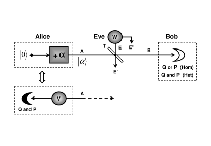
Figure 1: Coherent state protocols. Alice prepares a coherent state $\left|\alpha\right\rangle$ that Bob detects via a homodyne or heterodyne detector. A Gaussian (entangling cloner) attack by Eve is also shown. Note that preparing a coherent state (via modulating the vacuum) can be equivalently achieved by heterodyning one of the two modes of an EPR pair.

In the CV framework, collective Gaussian attacks represent the most powerful tool that today can be handled in the cryptoanalysis of Gaussian state protocols AcinNew ; CerfNew ; Renner ; Renner2 . In the most general definition of a collective attack, all the quantum systems used by Alice and Bob in a single run of the protocol are made to interact with a fresh ancillary system prepared by Eve. Then, all the output ancillas, coming from a large number of such single-run interactions, are subject to a final coherent measurement that is furthermore optimized upon all of Alice and Bob’s classical communications. In particular, the collective attack is Gaussian if the single-run interactions are Gaussian, i.e., corresponding to unitaries that preserve the Gaussian statistics of the states. Notice that for standard one-way QKD, a single run of the protocol corresponds to a single use of the channel. As a consequence, every collective Gaussian attack against one-way protocols results in a memoryless channel and, therefore, can be called a one-mode Gaussian attack. Since the quadratures encode independent variables $\{Q_{A},P_{A}\}$, the single-run Gaussian interactions do not need to mix the quadratures AcinNew ; CerfNew ; GrangNew ; RaulNew . As a consequence, the Gaussian interaction can be modelled by an entangling cloner Homo2 (see Fig. 1) where a beam splitter (of transmission $T$) mixes each signal mode $A$ with an ancillary mode $E$ belonging to an Einstein-Podolsky-Rosen (EPR) pair (see Appendix). Such an EPR pair is characterized by a variance $W$ and correlates the two output ancillary modes $E^{\prime},E^{\prime\prime}$ to be detected in the final coherent measurement. Notice that, from the point of view of Alice and Bob, this EPR pair simply reduces to an environmental thermal state $\rho_{E}$ with thermal number $\bar{n}_{E}=(W-1)/2$. A one-mode Gaussian attack can be therefore described by two parameters: transmission $T$ and variance $W$ or, equivalently, by $T$ and $N:=(W-1)(1-T)T^{-1}$, the latter being the excess noise of the channel. This parameter quantifies the amount of extra noise which is not referable to losses, i.e., the effect of the thermal noise scaled by the transmission Homo2 . The security thresholds against these powerful attacks can be expressed in terms of tolerable excess noise $\{N^{\blacktriangleright},N^{\blacktriangleleft}\}$ versus the transmission $T$ of the channel. For protocols $Hom$ and $Het$, these thresholds are displayed in Fig. 2 for DR and Fig. 3 for RR, and they confirm the results previously found in Refs. LCcollective ; LCcollective2 (see Appendix).

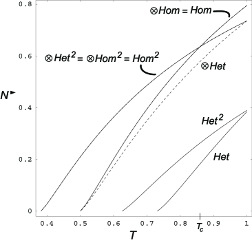
Figure 2: Security thresholds in direct reconciliation. The figure shows the tolerable excess noise $N^{\blacktriangleright}$ (in quantum shot-noise units) versus transmission $T$. Curves compare the various one-way and two-way protocols against one-mode Gaussian attacks $\{N,T\}$ in the limit of large modulation $(V\rightarrow+\infty)$.

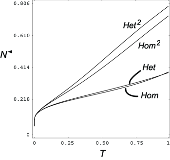
Figure 3: Security thresholds in reverse reconciliation. The figure shows the tolerable excess noise $N^{\blacktriangleleft}$ (in quantum shot-noise units) versus transmission $T$. Curves compare the individual one-way and two-way protocols against one-mode Gaussian attacks $\{N,T\}$ in the limit of large modulation $(V\rightarrow+\infty)$.

II From one-way to two-way protocols

The above coherent state protocols have been simply formulated in terms of prepare and measure (PM) schemes. Equivalently, they can be formulated as entanglement-based schemes, where Alice and Bob extract a key from the correlated outcomes of the measurements made upon two entangled modes (see Fig. 1). In fact, heterodyning one of the two entangled modes of an EPR pair (with variance $V$) is equivalent to remotely preparing a coherent state $\left|\alpha\right\rangle$ whose amplitude is randomly modulated by a Gaussian (with variance $V-1$) Estimators . In this dual representation of the protocol, Alice owns a physical resource which can be equivalently seen as an amount of energy $\sim V$ for modulation (in the PM representation) or as an amount of entanglement $\sim\log 2V$ to be distributed (in the entanglement-based representation). Because of this equivalence, the previous entanglement is also called virtual Estimators . In the above one-way protocols, all these physical resources are the monopoly of Alice and their sole purpose is the encoding of secret information. However, we can also consider a scenario where these resources are symmetrically distributed between Alice and Bob, and part of them is used to assist the encoding. This is achieved by combining Alice and Bob in a two-way quantum communication where Bob’s physical resources, to be generally intended as entanglement resources, assist the secret encoding of Alice, which is realized by unitary random modulations (see Fig. 4).

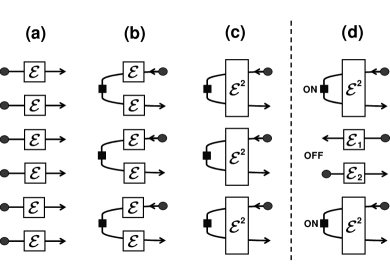
Figure 4: General structure of the one-way, two-way and hybrid protocols, together with their possible collective attacks. Circles and squares represent the physical resources available in the process. In particular, circles represent entanglement (possibly virtual) while squares are unitary modulations. In the inset (a), the basic one-way scheme is depicted, where all the resources are owned by Alice. In the insets (b) and (c), the physical resources are instead distributed between Alice and Bob, where Bob uses them for assisting while Alice for encoding (two-way scheme). Inset (d) shows the hybrid protocol where one-way’s (OFF) and two-way’s (ON) are randomly switched. All the insets also display Eve’s collective attacks. The inset (a) shows the collective attacks against one-way protocols (one-mode attacks). The insets (b) and (c) show instead the collective attacks against the two-way protocols. These are one-mode (or reducible two-mode) in the inset (b) while two-mode in the inset (c). Finally, inset (d) shows the effects of a two-mode attack on the hybrid protocol.

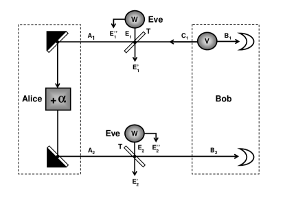
Figure 5: Two-way quantum communication scheme. Bob exploits an EPR pair to assist Alice’s encoding. He keeps one mode $B_{1}$ while sending the other one $C_{1}$ to Alice who, in turn, perfoms a stochastic phase-space displacement $+\alpha$. The resulting mode $A_{2}$ is then sent back to Bob. The final modes $B_{1}$ and $B_{2}$ are incoherently detected by means of two homodyne detectors ($Hom^{2}$ protocol) or two heterodyne detectors ($Het^{2}$ protocol). The figure also displays a one-mode Gaussian attack, where the forward mode $C_{1}$ (from Bob to Alice) and the backward one $A_{2}$ (from Alice to Bob) are subject to the action of entangling cloners.

Let us explicitly construct such a two-way quantum communication. In simple two-way generalizations, $Hom^{2}$ and $Het^{2}$, of the previous one-way protocols, $Hom$ and $Het$, Bob exploits an assisting EPR pair (with variance $V$) of which he keeps one mode $B_{1}$ while sending the other to Alice (see Fig. 5). Then, Alice encodes her information via Gaussian modulation (with variance $V-1$) by adding a stochastic amplitude $\alpha=(Q_{A}+iP_{A})/2$ to the received mode. Such a mode is then sent back to Bob, where it is detected together with the unsent mode $B_{1}$. Depending on the protocol, Bob will perform different detections on modes $B_{1}$ and $B_{2}$. In particular, for the $Hom^{2}$ protocol, Bob will detect the $\hat{Q}$ (or $\hat{P}$) quadrature of such modes (homodyne detections), while, for the $Het^{2}$ protocol, he will detect both $\hat{Q}$ and $\hat{P}$ (heterodyne detections). From the outcomes, Bob will finally construct an optimal estimator $X_{B}$ of Alice’s corresponding variable $X_{A}$, equal to $Q_{A}$ (or $P_{A}$) for $Hom^{2}$ and to the $\mathbb{R}^{2}$-vector $\{Q_{A},P_{A}\}$ for $Het^{2}$.

Since Bob’s decoding strategy consists in individual incoherent detections, these entanglement-assisted QKD schemes are actually equivalent to two-way schemes without entanglement, where Bob stochastically prepares a quantum state to be sequentially transmitted forward and backward in the channel. In fact, one can assume that Bob detects $B_{1}$ at the beginning of the quantum communication, so that the travelling mode $C_{1}$ is randomly prepared in a reference quantum state (which is squeezed for $Hom^{2}$ and coherent for $Het^{2}$). This reference state reaches Alice where stores the encoding transformation and, then, is finally detected by the second decoding measurement of Bob. Therefore, if we restrict Bob to incoherent detections (classical Bob), then the two-way schemes also possess a dual representation, where the assisting entanglement resource is actually virtual, i.e., can be replaced by an equivalent random modulation. In this dual (entanglement-free) representation, the advantage brought by the two-way quantum communication can be understood in terms of an iterated use of the uncertainty principle, where Eve is forced to produce a double perturbation of the same quantum channel. For instance, let us consider the $Het^{2}$ protocol in the absence of eavesdropping. By heterodyning mode $B_{1}$, Bob randomly prepares mode $C_{1}$ in a reference coherent state $\left|\beta\right\rangle$ containing a random modulation $\gamma$ known only to him. Then, Alice transforms this state into another coherent state $\left|\alpha+\beta\right\rangle$ which is sent back to Bob. By the subsequent heterodyne detection, Bob is able to estimate the total amplitude $\alpha+\beta$ and, therefore, to infer the signal $\alpha$ from his knowledge of $\beta$. If we now insert Eve in this scenario, we see that she must estimate both the reference $\beta$ and the masked signal $\alpha+\beta$ in order to access the signal $\alpha$. This implies attacking both the forward and the backward channel (see Fig. 5) and, since the noise of the first attack will perturb the second attack, we expect a non trivial security improvement in the process. Such an effect intuitively holds under the assumption of one-mode attacks (where the two paths are attacked incoherently) and it is indeed confirmed by our analysis. Quantitatively, we have tested the security performances of the two-way protocols against the one-mode Gaussian attacks $\{N,T\}$ and the corresponding security thresholds $N^{\blacktriangleright,\blacktriangleleft}=N^{\blacktriangleright,\blacktriangleleft}(T)$ are shown in Fig. 2 and Fig. 3 (see Appendix). For the two-way protocols, such thresholds relate the tolerable excess noise to the transmission in each use of the channel and, therefore, they are directly comparable with the thresholds of the corresponding one-way protocols. By comparing $Hom^{2}$ with $Hom$ and $Het^{2}$ with $Het$, one sees that the security thresholds are improved almost everywhere (the only exception being $Hom^{2}$ for $T>T_{c}\simeq 0.86$ in DR). Such a superadditive behavior is the central result of this work. Roughly speaking, even if two communication lines (e.g., two optical fibers) are too noisy for one-way QKD, they can be combined to enable a two-way QKD, as long as the quantum channel is memoryless.

In order to deepen our analysis on superadditivity, we also tested the previous one-way and two-way protocols when a classical Bob is replaced by a quantum Bob. This means that Bob is no longer limited to incoherent detections but can access a quantum memory storing all the modes involved in the quantum communication. Then, Bob performs a final optimal coherent measurement on all these modes in order to retrieve Alice’s information. Such a coherent measurement can be disjoint, i.e., designed to estimate a single quadrature for each encoding, or joint, i.e., designed to estimate both quadratures. Correspondingly, the modified one-way and two-way protocols will be denoted by $\otimes Hom$, $\otimes Het$, $\otimes Hom^{2}$ and $\otimes Het^{2}$. Notice that these collective protocols may not admit an equivalent entanglement-free representation (where Bob’s entanglement is replaced by a random modulation) if Bob’s coherent measurement cannot be reduced to incoherent detection. The corresponding security thresholds are shown in Fig. 2 (only DR can be compared, see Appendix). It is evident that superadditivity holds almost everywhere also for these collective schemes, the only exception being $\otimes Hom^{2}$ above the same critical value $T_{c}$ as before. We easily note that $\otimes Hom$ coincides with $Hom$, while $\otimes Hom^{2}$ coincides with $Hom^{2}$. Then, in the case of disjoint decoding, the optimal coherent measurement asymptotically coincides with a sequence of incoherent homodyne detections. As a consequence, the collective protocols ($\otimes Hom$ and $\otimes Hom^{2}$) collapse to the corresponding individual protocols ($Hom$ and $Hom^{2}$), where there is no need for a quantum memory. In particular, this proves that $\otimes Hom^{2}$ admits an entanglement-free representation where infinitely-squeezed states are sent to Alice through the forward path, and are then homodyned at the output of the backward path. The usage of quantum memories does better in the case of joint decoding, since $\otimes Het$ and $\otimes Het^{2}$ have much better performances than the corresponding individual protocols $Het$ and $Het^{2}$. As a consequence, no simple entanglement-free representation is known for $\otimes Het^{2}$.

III Hybrid protocols

We remark that our previous quantitative cryptoanalysis concerns one-mode Gaussian attacks, which are the cryptographic analog of a memoryless Gaussian channel. However, when a multi-way scheme is considered, a single run of the protocol no longer corresponds to a single use of the channel. As a consequence, the most general collective attack against a multi-way scheme, even if incoherent between separate runs, may involve quantum correlations between different channels. In general, an arbitrary collective attack against a two-way scheme can be called a two-mode attack. This is the general scenario of Fig. 4(c) where the action of this attack on a single round-trip of quantum communication is given by an arbitrary map $\mathcal{E}^{2}$. On the one hand, such an attack is said to be reducible to a one-mode attack if the map can be symmetrically decomposed as $\mathcal{E}^{2}=\mathcal{E}\circ\mathcal{E}$ (i.e., the attack can be described by the scenario of Fig. 4(b)) On the other hand, the two-mode attack is called irreducible if $\mathcal{E}^{2}\neq\mathcal{E}\circ\mathcal{E}$ (i.e., the attack of Fig. 4(c) cannot be described by Fig. 4(b)). The latter situation includes all attacks where some kind of correlation is exploited between the two paths, either if this correlation is classical (so that $\mathcal{E}^{2}=\mathcal{E}_{2}\circ\mathcal{E}_{1}$ with $\mathcal{E}_{1}\neq\mathcal{E}_{2}$) or truly quantum (so that $\mathcal{E}^{2}\neq\mathcal{E}_{2}\circ\mathcal{E}_{1}$ for every $\mathcal{E}_{1}$ and $\mathcal{E}_{2}$).

In order to detect and handle an irreducible attack, the previous two-way protocols, $Hom^{2}$ and $Het^{2}$, must be modified into hybrid forms that we denote by $Hom^{1,2}$ and $Het^{1,2}$. In this hybrid formulation, Alice randomly switches between a two-way scheme and the corresponding one-way scheme, where she simply detects the incoming mode and sends a new one back to Bob. We may describe this process by saying that Alice randomly closes (ON) and opens (OFF) the quantum communication circuit with Bob, the effective switching sequence being communicated at the end of the protocol (see Fig. 4(d)). By publicizing part of the exchanged data, Alice and Bob can perform tomography of the quantum channels in both the ON and OFF configurations. In particular, they can reconstruct the channel $\mathcal{E}^{2}$ affecting the two-way trip and the channels $\mathcal{E}_{1}$ and $\mathcal{E}_{2}$ affecting the forward and backward paths (see Fig. 4(d)). Then, they can check the reducibility conditions $\mathcal{E}_{1}=\mathcal{E}_{2}$ and $\mathcal{E}^{2}=\mathcal{E}_{2}\circ\mathcal{E}_{\alpha}\circ\mathcal{E}_{1}$, where $\mathcal{E}_{\alpha}(\rho)=\hat{D}(\alpha)\rho\hat{D}^{\dagger}(\alpha)$ is Alice’s publicized encoding map. If such conditions are satisfied then the two-mode attack is reducible, i.e., Alice and Bob have excluded every kind of quantum and classical correlation between the two paths of the quantum communication (see Appendix for an explicit description). In such a case, the honest users can therefore exploit the superadditivity of the two-way quantum communication. If the previous reducibility conditions are not met, then the honest users can always exploit the instances of one-way quantum communication. Notice that the verification of the reducibility conditions is rather easy in the Gaussian case, where the channels can be completely reconstructed by analyzing the first and second statistical moments of the output states. Also notice that the reducibility conditions exclude every kind of quantum impersonation attack Dusek , where Eve short-circuits the channels of the two-way quantum communication.

In conclusion, the hybrid protocols constitute a safe implementation of two-way protocols, at least in the presence of collective Gaussian attacks (one-mode or two-mode). In the hybrid formulation, Alice and Bob can in fact optimize their security on both one-way and two-way quantum communication. The ON-OFF manipulation of the quantum communication can be interpreted as if Alice had two orthogonal bases to choose from during the key distribution process. In the presence of this randomization, Eve is not able to optimize her Gaussian attack with respect to both kinds of quantum communication and the trusted parties can always make the a posteriori optimal choice. As a natural development of these results, one can consider a situation where Bob also performs a random and independent ON-OFF manipulation of the quantum communication. Such a scheme naturally leads to instances of $n$-way quantum communication (with $n>2$) whose security properties would be interesting to inspect in future work. In general, our results pave the way for future investigations in the domain of secure multiple quantum communications, where quantum communication circuits can in principle grow to higher and higher complexity.

IV Acknowledgements

The research of S. Pirandola was supported by a Marie Curie Fellowship within the 6th European Community Framework Programme (Contract No. MOIF-CT-2006-039703). S. Pirandola thanks CNISM for hospitality at the University of Camerino and Gaetana Spedalieri for her moral and logistic support. S. Lloyd was supported by the W.M. Keck foundation center for extreme quantum information theory (xQIT).

Appendix A Appendix

In this technical section, we first review some basic information about Gaussian states. Then, we exhibit the general expressions for the secret-key rates (in both direct and reverse reconciliation) when the various protocols are subject to one-mode Gaussian attacks. In the following subsections, we explicitly compute these secret-key rates for all the one-way and two-way protocols. From these quantities we derive the security thresholds shown in the paper. Finally, in the last subsection, we give the explicit description of a general two-mode attack and we analyze the conditions for its reducibility. This last analysis shows the security of the hybrid protocols against collective Gaussian attacks.

A.1 Basics of Gaussian states

A bosonic system of $n$ modes can be described by a quadrature row-vector $\mathbf{\hat{Y}}:=(\hat{Q}_{1},\hat{P}_{1},\ldots,\hat{Q}_{n},\hat{P}_{n})$ satisfying $[\hat{Y}_{l},\hat{Y}_{m}]=2i\Omega_{lm}$ ($1\leq l,m\leq 2n$), where

$$\mathbf{\Omega}:=\bigoplus\limits_{k=1}^{n}\left(\begin{array}[]{cc}0&1\\ -1&0\end{array}\right)$$ (1)

defines a symplectic form. A bosonic state $\rho$ is called Gaussian if its statistics is Gaussian EisertGauss ; GaussianStates . In such a case, the state $\rho$ is fully characterized by its displacement $\langle\mathbf{\hat{Y}}\rangle=\mathrm{Tr}(\mathbf{\hat{Y}}\rho)$ and correlation matrix (CM) $\mathbf{V}$, whose generic element is defined by $V_{lm}:=\langle\hat{Y}_{l}\hat{Y}_{m}+\hat{Y}_{m}\hat{Y}_{l}\rangle/2-\langle\hat{Y}_{l}\rangle\langle\hat{Y}_{m}\rangle$ with diagonal terms $V_{ll}=\langle\hat{Y}_{l}^{2}\rangle-\langle\hat{Y}_{l}\rangle^{2}:=V(\hat{Y}_{l})$ express the variances of the quadratures. According to Williamson’s theorem Williamson , every CM $\mathbf{V}$ can be put in diagonal form by means of a symplectic transformation, i.e., there exists a matrix $\mathbf{S}$, satisfying $\mathbf{\mathbf{S}}^{T}\mathbf{\Omega S}=\mathbf{\Omega}$, such that $\mathbf{\mathbf{S}}^{T}\mathbf{VS}=\mathbf{\Delta(}\nu_{1},\nu_{1},\cdots,\nu_{n},\nu_{n})$, where $\mathbf{\Delta}$ denotes a diagonal matrix. The set of real values $\boldsymbol{\nu}:=\{\nu_{1},\cdots,\nu_{n}\}$ is called symplectic eigenspectrum of the CM and provides compact ways to express fundamental properties of the corresponding Gaussian state. In particular, the Von Neumann entropy $S(\rho):=-\mathrm{Tr}\left(\rho\log\rho\right)$ of a Gaussian state $\rho$ can be expressed in terms of the symplectic eigenvalues by the formula Entropia

$$S(\rho)=\sum\limits_{k=1}^{n}g(\nu_{k})~{},$$ (2)

where

$$g(\nu):=\tfrac{\nu+1}{2}\log\tfrac{\nu+1}{2}-\tfrac{\nu-1}{2}\log\tfrac{\nu-1}{2}$$

$$\rightarrow\log\tfrac{e\nu}{2}+O(\nu^{-1})\text{~{}~{}for }\nu\gg 1\text{~{}.}$$ (3)

Here, the information unit is the bit if $\log=\log_{2}$ or the nat if $\log=\ln$.

An example of a Gaussian state is the two-mode squeezed vacuum state QObook (or EPR source) whose CM takes the form

$$\mathbf{V}_{EPR}(V)=\left(\begin{array}[]{cc}V\mathbf{I}&\sqrt{V^{2}-1}\mathbf{Z}\\ \sqrt{V^{2}-1}\mathbf{Z}&V\mathbf{I}\end{array}\right),$$ (4)

where $\mathbf{Z}:=\mathbf{\Delta}(1,-1)$ and $\mathbf{I}:=\mathbf{\Delta}(1,1)$. In Eq. (4) the variance $V$ fully characterizes the EPR source QObook . On the one hand, it quantifies the amount of entanglement which is distributed between Alice and Bob, providing a log-negativity LogNeg equal to

$$E_{\mathcal{N}} = \max\left\{0,-\tfrac{1}{2}\log(2V^{2}-1-2V\sqrt{V^{2}-1})\right\}$$ (5)

$$\rightarrow \log 2V+O(V^{-2})\text{~{}~{}for }V\gg 1\text{~{}.}$$

On the other hand, it quantifies the amount of energy which is distributed to the parties, since the reduced thermal states $\rho_{A}:=\mathrm{Tr}_{B}(\rho)$ and $\rho_{B}:=\mathrm{Tr}_{A}(\rho)$ have mean excitation numbers equal to $(V-1)/2$.

A.2 General expressions for the secret-key rates

The various protocols differ for the number of paths ($1$ or $2$) and the decoding method, which can be joint, disjoint, individual or collective. In particular, when decoding is disjoint the relevant secret variable $X$ is $Q\in\mathbb{R}$ (or $P\in\mathbb{R}$, equivalently). When decoding is joint, the relevant secret variable $X$ is $\{Q,P\}\in\mathbb{R}^{2}$. Under the assumption of one-mode Gaussian attacks, the individual protocols ($Hom,Het,Hom^{2},Het^{2}$) have the following secret-key rates for DR ($\blacktriangleright$) and RR ($\blacktriangleleft$) DWrate ; DWrate2

$$R^{\blacktriangleright}:=I(X_{A}:X_{B})-I(X_{A}:E)~{},$$ (6)

$$R^{\blacktriangleleft}:=I(X_{A}:X_{B})-I(X_{B}:E)~{}.$$ (7)

In these formulae, $I(X_{A}:X_{B}):=H(X_{B})-H(X_{B}|X_{A})$ is the classical mutual information between Alice and Bob’s variables $X_{A}$ and $X_{B}$, with $H(X_{B})=(1/2)\log V(X_{B})$ and $H(X_{B}|X_{A})=(1/2)\log V(X_{B}|X_{A})$ being the total and conditional Shannon entropies Shannon . The term

$$I(X_{K}:E):=H(E)-H(E|X_{K})$$ (8)

is the Holevo information HInfo between Eve ($E$) and the honest user $K=A,B$ (i.e., Alice or Bob). Here, $H(E):=S(\rho_{E})$ is the Von Neumann entropy of Eve’s state $\rho_{E}$ and $H(E|X_{K})$ is the Von Neumann entropy conditioned to the classical communication of $X_{K}$. For the collective protocols ($\otimes Hom,\otimes Het,\otimes Hom^{2},\otimes Het^{2}$) we have instead

$$R^{\blacktriangleright}:=I(X_{A}:B)-I(X_{A}:E)~{},$$ (9)

and

$$R^{\blacktriangleleft}:=I(X_{A}:B)-I(B:E)~{},$$ (10)

where $I(X_{A}:B)$, $I(X_{A}:E)$ are Holevo informations, and

$$I(B:E):=H(B)+H(E)-H(B,E)$$ (11)

is the quantum mutual information between Bob and Eve. By setting $R=0$ in the above Eqs. (6), (7), (9) and (10) one finds the security thresholds for the corresponding protocols. Notice that the Holevo information of Eq. (8) provides an upper bound to Eve’s accessible information. In the case of collective protocols, Alice and Bob are able to reach the Holevo bound $I(X_{A}:B)$ only asymptotically. This is possible if Alice communicates to Bob the optimal collective measurement to be made compatible with the generated sequence of signal states and the detected noise in the channel. Such a measurement will be an asymptotic projection on the codewords of a random quantum code as foreseen by the Holevo–Schumacher–Westmoreland (HSW) theorem HSW ; HSW2 . Though such a measurement is highly complex, it is in principle possible and the study of the collective DR secret-key rate of Eq. (9) does make sense (it is also connected to the notion of private classical capacity of Ref. Privacy ). On the other hand, the quantum mutual information of Eq. (11) provides a bound which is too large in general, preventing a comparison between the collective protocols in RR.

A.3 Secret-key rates of the one-way protocols

In the one-way protocols, Alice encodes two independent Gaussian variables $Q_{A},P_{A}$ in the quadratures $\hat{Q}_{A},\hat{P}_{A}$ of a signal mode $A$, i.e., $\hat{Q}_{A}=Q_{A}+\hat{Q}_{A}|Q_{A}$ and $\hat{P}_{A}=P_{A}+\hat{P}_{A}|P_{A}$. Here, the quantum variables $\hat{Q}_{A},\hat{P}_{A}$ have a global modulation $V$, given by the sum of the classical modulation $V(Q_{A})=V(P_{A})=V-1$ and the quantum shot-noise $V(\hat{Q}_{A}|Q_{A})=V(\hat{P}_{A}|P_{A})=1$. On the other hand, Eve has an EPR source $\mathbf{V}_{EPR}(W)$ which distributes entanglement between modes $E$ and $E^{\prime\prime}$. The spy mode $E$ is then mixed with the signal mode $A$ via a beam splitter of transmission $T$, and the output modes, $B$ and $E^{\prime}$, are received by Eve and Bob, respectively (see Fig. 1). Let us first consider the case of collective protocols ($\otimes Hom,\otimes Het$), where Bob performs a coherent detection on all the collected modes $B$ in order to decode $X_{A}=Q_{A}$ (for $\otimes Hom$) or $X_{A}=\{Q_{A},P_{A}\}$ (for $\otimes Het$). For an arbitrary triplet $\{V,W,T\}$, the quadratures of the output modes, $B$ and $E^{\prime}$, have variances

$$V(\hat{Q}_{B})=V(\hat{P}_{B})=(1-T)W+TV:=b_{V}~{},$$ (12)

$$V(\hat{Q}_{E^{\prime}})=V(\hat{P}_{E^{\prime}})=(1-T)V+TW:=e_{V}~{},$$ (13)

and conditional variances

$$V(\hat{Q}_{B}|Q_{A})=V(\hat{P}_{B}|P_{A})=(1-T)W+T=b_{1}~{},$$ (14)

$$V(\hat{Q}_{E^{\prime}}|Q_{A})=V(\hat{P}_{E^{\prime}}|P_{A})=(1-T)+TW=e_{1}~{}.$$ (15)

Globally, the CMs of the output states $\rho_{B}$ (of Bob), $\rho_{E^{\prime}E^{\prime\prime}}:=\rho_{E}$ (of Eve) and $\rho_{E^{\prime}E^{\prime\prime}B}:=\rho_{EB}$ (of Eve and Bob) are given by

$$\mathbf{V}_{B}(V,V)=\mathbf{\Delta(}b_{V},b_{V})~{},$$ (16)

$$\mathbf{V}_{E}(V,V)=\begin{pmatrix}\mathbf{\Delta[}e_{V},e_{V}]&\varphi\mathbf{Z}\\ \varphi\mathbf{Z}&W\mathbf{I}\end{pmatrix}~{},$$ (17)

and

$$\mathbf{V}_{EB}=\left(\begin{array}[]{cc}\mathbf{V}_{E}&\mathbf{F}\\ \mathbf{F}^{T}&\mathbf{V}_{B}\end{array}\right)~{},~{}\mathbf{F:}=\binom{\mu\mathbf{I}}{\theta\mathbf{Z}}~{},$$ (18)

where

$$\varphi:=[T(W^{2}-1)]^{1/2}~{},~{}\mu:=(W-V)[(1-T)T]^{1/2}~{},$$ (19)

and

$$\theta:=[(1-T)(W^{2}-1)]^{1/2}~{}.$$ (20)

The CMs of Bob ($B$) and Eve ($E$), conditioned to Alice’s variable $X_{A}$, are instead equal to

$$\mathbf{V}_{K|Q_{A}}=\mathbf{V}_{K}(1,V)~{},~{}\mathbf{V}_{K|Q_{A},P_{A}}=\mathbf{V}_{K}(1,1)~{},$$ (21)

where $K=B,E.$ For $T\neq 0,1$ and $V\gg 1$, the symplectic spectra of all the previous CMs are given by:

$$\boldsymbol{\nu}_{B} \rightarrow \{TV\}~{},$$ (22)

$$\boldsymbol{\nu}_{B|Q_{A}} \rightarrow \{\sqrt{b_{1}TV}\}~{},$$ (23)

$$\boldsymbol{\nu}_{B|Q_{A},P_{A}} \rightarrow \{b_{1}\}~{},$$ (24)

$$\boldsymbol{\nu}_{E} \rightarrow \{(1-T)V,W\}~{},$$ (25)

$$\boldsymbol{\nu}_{E|Q_{A}} \rightarrow \{\sqrt{e_{1}(1-T)V},\sqrt{Wb_{1}/e_{1}}\}~{},$$ (26)

$$\boldsymbol{\nu}_{E|Q_{A},P_{A}} \rightarrow \{b_{1},1\}~{},$$ (27)

$$\boldsymbol{\nu}_{BE} \rightarrow \{V,1,1\}~{}.$$ (28)

By using Eqs. (2) and (3), we then compute all the Von Neumann entropies to be used in the quantities $I(X_{A}:B),$ $I(X_{A}:E)$ and $I(B:E)$ of Eqs. (9) and (10). After some algebra we get the following asymptotic rates for the one-way collective protocols

$$R^{\blacktriangleright}[\otimes Het]=\log\tfrac{T}{1-T}-g(W)~{},$$ (29)

$$R^{\blacktriangleright}[\otimes Hom]=\tfrac{1}{2}\log\tfrac{Te_{1}}{(1-T)b_{1}}+g\left(\sqrt{\tfrac{Wb_{1}}{e_{1}}}\right)-g(W)~{}\text{,}$$ (30)

and

$$R^{\blacktriangleleft}[\otimes Het]=\log\tfrac{1}{1-T}-g(W)-g(b_{1})~{},$$ (31)

while $R^{\blacktriangleleft}[\otimes Hom]\rightarrow-\infty$, because of the too large bound provided by $I(B:E)$ in this case.

Let us now consider the individual one-way protocols ($Hom,Het$). Bob’s output variable is $Q_{B}=\hat{Q}_{B}$ for $Hom$, and

$$\{Q_{B},P_{B}\}=2^{-1/2}\{\hat{Q}_{B}+\hat{Q}_{0},\hat{P}_{B}-\hat{P}_{0}\}$$ (32)

for $Het$ (with $\hat{Q}_{0},\hat{P}_{0}$ belonging to the vacuum). From Eqs. (12) and (14), we can calculate the variances $V(X_{B})$ and $V(X_{B}|X_{A})$ that provide the non-computed term $I(X_{A}:X_{B})$ in Eq. (6). Then, we get the following asymptotic rates in DR

$$R^{\blacktriangleright}[Hom]=R^{\blacktriangleright}[\otimes Hom]\text{~{},}$$ (33)

and

$$R^{\blacktriangleright}[Het]=\log\tfrac{2T}{e(1-T)(1+b_{1})}+g(b_{1})-g(W)~{}.$$ (34)

In order to derive the RR rates from Eq. (7) we must evaluate

$$I(X_{B}:E)=H(E)-H(E|X_{B})~{},$$ (35)

where $H(E|X_{B})$ is computed from the spectrum $\boldsymbol{\nu}_{E|X_{B}}$ of the conditional CM $\mathbf{V}_{E|X_{B}}$. In RR, Eve’s quantum variables

$$\hat{Y}_{E}:=(\hat{Q}_{E^{\prime}},\hat{P}_{E^{\prime}},\hat{Q}_{E^{\prime\prime}},\hat{P}_{E^{\prime\prime}})$$ (36)

must be conditioned to the Bob’s classical variable $X_{B}.$ This is equivalent to constructing, from $X_{B}$, the optimal linear estimators $\hat{Y}_{E}^{(X_{B})}$ of $\hat{Y}_{E}$, in such a way that the residual conditional variables

$$\hat{Y}_{E}|X_{B}:=\hat{Y}_{E}-\hat{Y}_{E}^{(X_{B})}$$ (37)

have minimal entropy $H(E|X_{B})$. For the $Hom$ protocol, Bob’s variable $X_{B}=Q_{B}$ can be used to estimate the $\hat{Q}$ quadratures only. Then, let Bob estimate $\hat{Y}_{E}$ by

$$\hat{Y}_{E}^{(Q_{B})}=(q^{\prime}Q_{B},0,q^{\prime\prime}Q_{B},0)~{},$$ (38)

so that the conditional variables are given by

$$\hat{Y}_{E}|Q_{B}=(\hat{Q}_{E^{\prime}}-q^{\prime}Q_{B},\hat{P}_{E^{\prime}},\hat{Q}_{E^{\prime\prime}}-q^{\prime\prime}Q_{B},\hat{P}_{E^{\prime\prime}})~{}.$$ (39)

For $T\neq 0,1$ and $V\gg 1$, the optimal estimators are given by

$$q^{\prime}=-\sqrt{(1-T)/T}~{},$$ (40)

and $q^{\prime\prime}=0$. The corresponding conditional spectrum

$$\boldsymbol{\nu}_{E|Q_{B}}\rightarrow\{\sqrt{VW(1-T)/T},1\}$$ (41)

minimizes $H(E|Q_{B})$ and leads to the asymptotic rate

$$R^{\blacktriangleleft}[Hom]=\tfrac{1}{2}\log\tfrac{W}{(1-T)b_{1}}-g(W)~{}.$$ (42)

For the $Het$ protocol, Bob’s variable $X_{B}=\{Q_{B},P_{B}\}$ enables him to estimate both the $\hat{Q}$ and $\hat{P}$ quadrature, by constructing the $\hat{Y}_{E}$-linear estimator

$$\hat{Y}_{E}^{(Q_{B},P_{B})}=(q^{\prime}Q_{B},p^{\prime}P_{B},q^{\prime\prime}Q_{B},p^{\prime\prime}P_{B})~{}.$$ (43)

For $T\neq 0,1$ and $V\gg 1$, the optimal choice corresponds to

$$q^{\prime}=p^{\prime}=-\sqrt{2(1-T)/T}~{},$$ (44)

and $q^{\prime\prime}=p^{\prime\prime}=0$, which gives

$$\boldsymbol{\nu}_{E|Q_{B},P_{B}}\rightarrow\{(1-T+b_{1})/T,1\}~{},$$ (45)

and leads to the asymptotic rate

$$R^{\blacktriangleleft}[Het]=\log\tfrac{2T}{e(1-T)(1+b_{1})}+g\left(\tfrac{1-T+b_{1}}{T}\right)-g(W)~{}.$$ (46)

A.4 Secret-key rates of the two-way protocols

In the EPR formulation of the two-way protocols (see Fig. 5), Bob assists the encoding via an EPR source $\mathbf{V}_{EPR}(V)$ that distributes entanglement between mode $B_{1}$, which is kept, and mode $C_{1}$, which is sent in the channel and undergoes the action of an entangling cloner $(T,W):C_{1}\rightarrow A_{1}$. On the perturbed mode $A_{1}$, Alice performs a Gaussian modulation by adding a stochastic amplitude $\alpha=(Q_{A}+iP_{A})/2$ with $V(Q_{A})=V(P_{A})=\bar{V}$ and $\left\langle Q_{A}P_{A}\right\rangle=0$. The modulated mode $A_{2}$ is then sent back through the channel, where it undergoes the action of a second entangling cloner $(T,W):A_{2}\rightarrow B_{2}$, where the output mode $B_{2}$ is finally received by Bob. Let us first consider the collective two-way protocols ($\otimes Hom^{2},\otimes Het^{2}$), where Bob performs an optimal coherent measurement upon all the collected modes $B_{1},B_{2}$ in order to decode $X_{A}=Q_{A}$ (for $\otimes Hom^{2}$) or $X_{A}=\{Q_{A},P_{A}\}$ (for $\otimes Het^{2}$). For an arbitrary quadruplet $\{\bar{V},V,W,T\}$, the CMs of the output states $\rho_{B_{1}B_{2}}:=\rho_{B}$ (of Bob) and $\rho_{E_{1}^{\prime}E_{1}^{\prime\prime}E_{2}^{\prime}E_{2}^{\prime\prime}}:=\rho_{E}$ (of Eve) are given by

$$\mathbf{V}_{B}(\bar{V},\bar{V})=\left(\begin{array}[]{cc}V\mathbf{I}&T\sqrt{V^{2}-1}\mathbf{Z}\\ T\sqrt{V^{2}-1}\mathbf{Z}&\boldsymbol{\Lambda}_{B}(\bar{V},\bar{V})\end{array}\right)~{},$$ (47)

and

$$\mathbf{V}_{E}(\bar{V},\bar{V})=\left(\begin{array}[]{cccc}e_{V}\mathbf{I}&\varphi\mathbf{Z}&\mu^{\prime}\mathbf{I}&\mathbf{0}\\ \varphi\mathbf{Z}&W\mathbf{I}&\theta^{\prime}\mathbf{Z}&\mathbf{0}\\ \mu^{\prime}\mathbf{I}&\theta^{\prime}\mathbf{Z}&\boldsymbol{\Lambda}_{E}(\bar{V},\bar{V})&\varphi\mathbf{Z}\\ \mathbf{0}&\mathbf{0}&\varphi\mathbf{Z}&W\mathbf{I}\end{array}\right)~{},$$ (48)

where

$$\boldsymbol{\Lambda}_{B}(\bar{V},\bar{V}):=[T^{2}V+(1-T^{2})W]\mathbf{I}+T\mathbf{\Delta(}\bar{V},\bar{V})~{},$$ (49)

and

$$\boldsymbol{\Lambda}_{E}(\bar{V},\bar{V}):=\gamma\mathbf{I+}(1\mathbf{-}T)\mathbf{\Delta(}\bar{V},\bar{V})~{},$$ (50)

with

$$\mu^{\prime}:=-\sqrt{1-T}\mu~{},~{}\theta^{\prime}:=-\sqrt{1-T}\theta~{},$$ (51)

and

$$\gamma:=T(1-T)V+(1-T)^{2}W+TW~{}.$$ (52)

The CMs of Bob ($B$) and Eve ($E$), conditioned to Alice’s variable $X_{A}$, are instead equal to

$$\mathbf{V}_{K|Q_{A}}=\mathbf{V}_{K}(0,\bar{V})~{},~{}\mathbf{V}_{K|Q_{A},P_{A}}=\mathbf{V}_{K}(0,0)~{},$$ (53)

for $K=B,E$. Let us consider identical resources between Alice and Bob, i.e., $\bar{V}=V-1$. Then, for $T\neq 0,1$ and $V\gg 1$, all the symplectic spectra are given by:

$$\boldsymbol{\nu}_{B} \rightarrow \{f_{1}V,f_{2}V\}~{},$$ (54)

$$\boldsymbol{\nu}_{B|Q_{A}} \rightarrow \{\varsigma V,\varsigma^{-1}\sqrt{T(1-T^{2})WV}\}~{},$$ (55)

$$\boldsymbol{\nu}_{B|Q_{A},P_{A}} \rightarrow \{(1-T^{2})V,W\}~{},$$ (56)

$$\boldsymbol{\nu}_{E} \rightarrow \{h_{1}V,h_{2}V,W,W\}~{},$$ (57)

$$\boldsymbol{\nu}_{E|Q_{A}} \rightarrow \{\upsilon(1-T)V,\tfrac{\sqrt{(1-T^{2})WV}}{\upsilon},W,1\}~{},$$ (58)

$$\boldsymbol{\nu}_{E|Q_{A},P_{A}} \rightarrow \{(1-T^{2})V,W,1,1\}~{},$$ (59)

where $f_{1}f_{2}=T$, $h_{1}h_{2}=(1-T)^{2}$ and

$$\varsigma:=[1+T^{2}(T^{2}+T-2)]^{1/2}~{},~{}\upsilon:=[1+3T+T^{2}]^{1/2}~{}.$$ (60)

By means of Eqs. (2) and (3), we compute all the Von Neumann entropies to be used in Eq. (9), and we get the asymptotic rates

$$R^{\blacktriangleright}[\otimes Hom^{2}]=\tfrac{1}{2}\log\tfrac{T}{(1-T)^{2}}-g(W)~{},$$ (61)

and

$$R^{\blacktriangleright}[\otimes Het^{2}]=2R^{\blacktriangleright}[\otimes Hom^{2}]~{}.$$ (62)

Clearly these rates imply the same DR threshold $N^{\blacktriangleright}=N^{\blacktriangleright}(T)$ for $\otimes Hom^{2}$ and $\otimes Het^{2}$, as is shown in Fig. 2. The derivation of $R^{\blacktriangleleft}[\otimes Het^{2}]$ and $R^{\blacktriangleleft}[\otimes Hom^{2}]$ is here omitted because of the trivial negative divergence caused by $I(B:E).$

Let us now consider the individual two-way protocols $Hom^{2}$ and $Het^{2}$ in DR. For the $Hom^{2}$ protocol, Bob decodes $Q_{A}$ by constructing the output variable $Q_{B}:=Q_{B_{2}}-TQ_{B_{1}}$ from the measurements of $\hat{Q}_{B_{1}}$ and $\hat{Q}_{B_{2}}$. In fact, since $\hat{Q}_{B_{1}}\rightarrow\hat{Q}_{C_{1}}$ (for $V\gg 1$) and

$$\hat{Q}_{B_{2}}=\sqrt{T}Q_{A}+T\hat{Q}_{C_{1}}+\sqrt{1-T}(\sqrt{T}\hat{Q}_{E_{1}}+\hat{Q}_{E_{2}})~{},$$ (63)

we asymptotically have

$$Q_{B}\rightarrow\sqrt{T}Q_{A}+\delta Q~{},$$ (64)

with

$$\delta Q:=\sqrt{1-T}(\sqrt{T}\hat{Q}_{E_{1}}+\hat{Q}_{E_{2}})~{}.$$ (65)

From $V(Q_{B})$ and $V(Q_{B}|Q_{A})$ we easily compute $I(Q_{A}:Q_{B})$ to be used in Eq. (6). It is then easy to check that the asymptotic DR rate satisfies

$$R^{\blacktriangleright}[Hom^{2}]=R^{\blacktriangleright}[\otimes Hom^{2}]~{}.$$ (66)

For the $Het^{2}$ protocol, Bob measures

$$\left\{\begin{array}[]{l}\hat{q}_{-}=2^{-1/2}(\hat{Q}_{B_{1}}-\hat{Q}_{0})~{},\\ \hat{p}_{+}=2^{-1/2}(\hat{P}_{B_{1}}+\hat{P}_{0})~{},\end{array}\right.$$ (67)

from the first heterodyne on $B_{1}$, and

$$\left\{\begin{array}[]{l}\hat{Q}_{-}=2^{-1/2}(\hat{Q}_{B_{2}}-\hat{Q}_{0^{\prime}})~{},\\ \hat{P}_{+}=2^{-1/2}(\hat{P}_{B_{2}}+\hat{P}_{0^{\prime}})~{},\end{array}\right.$$ (68)

from the second one upon $B_{2}$. Then, Bob decodes $\{Q_{A},P_{A}\}$ via the variables

$$\left\{\begin{array}[]{l}Q_{B}:=Q_{-}-Tq_{-}~{},\\ P_{B}:=P_{+}+Tp_{+}~{}.\end{array}\right.$$ (69)

In fact, for $T\neq 0,1$ and $V\gg 1$, we have

$$Q_{B}\rightarrow\sqrt{T/2}Q_{A}+\delta Q^{\prime}~{},~{}P_{B}\rightarrow\sqrt{T/2}P_{A}+\delta P~{},$$ (70)

with

$$\delta Q^{\prime}:=2^{-1/2}(\delta Q+T\hat{Q}_{0}-\hat{Q}_{0^{\prime}})~{},$$ (71)

and

$$\delta P:=2^{-1/2}[\sqrt{1-T}(\sqrt{T}\hat{P}_{E_{1}}+\hat{P}_{E_{2}})+T\hat{P}_{0}+\hat{P}_{0^{\prime}}]~{}.$$ (72)

From $V(X_{B})=V(Q_{B})V(P_{B})$ and $V(X_{B}|X_{A})=V(Q_{B}|Q_{A})V(P_{B}|P_{A})$ we then compute $I(X_{A}:X_{B})$ and the consequent asymptotic DR rate

$$R^{\blacktriangleright}[Het^{2}]=\log\tfrac{2T(1+T)}{e(1-T)[1+T^{2}+(1-T^{2})W]}-g(W)~{}.$$ (73)

Let us now consider $Hom^{2}$ and $Het^{2}$ in RR. In order to derive the corresponding rates from Eq. (7), we must again compute $H(E|X_{B})$ from the spectrum of the conditional CM $\mathbf{V}_{E|X_{B}}$, where Eve’s quantum variables

$$\hat{Y}_{E}:=(\hat{Q}_{E_{1}^{\prime}},\hat{P}_{E_{1}^{\prime}},\hat{Q}_{E_{1}^{\prime\prime}},\hat{P}_{E_{1}^{\prime\prime}},\hat{Q}_{E_{2}^{\prime}},\hat{P}_{E_{2}^{\prime}},\hat{Q}_{E_{2}^{\prime\prime}},\hat{P}_{E_{2}^{\prime\prime}})$$ (74)

are conditioned to Bob’s output variable $X_{B}$. Of course, this is again equivalent to finding the optimal linear estimators $\hat{Y}_{E}^{(X_{B})}$ of $\hat{Y}_{E}$. For the $Hom^{2}$ protocol where $X_{B}=Q_{B}$, the linear estimators of $\hat{Y}_{E}$ take the form

$$\hat{Y}_{E}^{(Q_{B})}:=(q_{1}^{\prime}Q_{B},0,q_{1}^{\prime\prime}Q_{B},0,q_{2}^{\prime}Q_{B},0,q_{2}^{\prime\prime}Q_{B},0)~{}.$$ (75)

For $T\neq 0,1$ and $V\gg 1$, the optimal ones are given by$\ q_{1}^{\prime}=q_{1}^{\prime\prime}=q_{2}^{\prime\prime}=0$ and $q_{2}^{\prime}=-\sqrt{(1-T)/T}$. The corresponding conditional spectrum is given by

$$\boldsymbol{\nu}_{E|Q_{B}}\rightarrow\{m_{1}V,m_{2}\sqrt{V},W,1\}~{},$$ (76)

with

$$m_{1}m_{2}=[T^{-1}(1-T)^{3}(1+T^{3})W]^{1/2}~{}.$$ (77)

This leads to the asymptotic rate

$$R^{\blacktriangleleft}[Hom^{2}]=\tfrac{1}{2}\log\tfrac{1-T+T^{2}}{(1-T)^{2}}-g(W)~{}.$$ (78)

For the $Het^{2}$ protocol, where $X_{B}=\{Q_{B},P_{B}\}$, we have

$$\hat{Y}_{E}^{(Q_{B},P_{B})}:=$$

$$(q_{1}^{\prime}Q_{B},p_{1}^{\prime}P_{B},q_{1}^{\prime\prime}Q_{B},p_{1}^{\prime\prime}P_{B},q_{2}^{\prime}Q_{B},p_{2}^{\prime}P_{B},q_{2}^{\prime\prime}Q_{B},p_{2}^{\prime\prime}P_{B})~{}.$$ (79)

For $T\neq 0,1$ and $V\gg 1$, the optimal estimators are given by

$$q_{2}^{\prime}=p_{2}^{\prime}=-\sqrt{2(1-T)/T}~{},$$ (80)

and

$$q_{1}^{\prime}=p_{1}^{\prime}=q_{1}^{\prime\prime}=p_{1}^{\prime\prime}=q_{2}^{\prime\prime}=p_{2}^{\prime\prime}=0~{}.$$ (81)

The corresponding conditional spectrum is given by

$$\boldsymbol{\nu}_{E|Q_{B},P_{B}}\rightarrow\{n_{1},n_{2},n_{3},(1-T^{2})V\}~{},$$

where

$$n_{1}n_{2}n_{3}=\frac{[1+T^{3}+(1-T)(1+T^{2})W]W}{T(1+T)}~{}.$$ (82)

This spectrum leads to the final asymptotic rate

$$R^{\blacktriangleleft}[Het^{2}]=\log\tfrac{2T(1+T)}{e(1-T)[1+T^{2}+(1-T^{2})W]}$$

$$+\sum\limits_{i=1}^{3}g(n_{i})-2g(W)~{}.$$ (83)

A.5 Structure of two-mode attacks

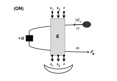
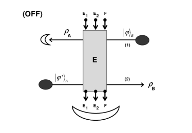
Figure 6: General two-mode attack against a hybrid protocol (displayed in both the ON and OFF configuration). The two paths of the quantum communication interact with a supply of ancillas that can always be divided into three blocks $E_{1},E_{2}$ and $F$.

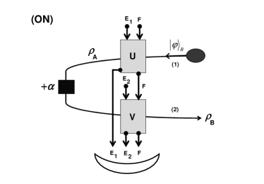
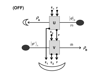
Figure 7: Cascade form of the two-mode attack. In the first unitary $\hat{U}$, two blocks of ancillas $E_{1}$ and $F$ interact with the forward path (labelled by 1). One output $E_{1}$ is sent to the final coherent detection while the other one $F$ is taken as input for the second unitary $\hat{V}$. Such a unitary makes the backward path (labelled by 2) interact with $F$ (coming from $\hat{U}$) and another block of fresh ancillas $E_{2}$. The corresponding outputs of $F$ and $E_{2}$ are then sent to the final coherent detection.

Let us describe the effects of a general two-mode attack when Alice and Bob adopt the hybrid protocol. In the hybrid protocol, Bob sends a modulated pure state $\left|\varphi\right\rangle_{B}$, which is coherent for $Het^{1,2}$ and squeezed for $Hom^{1,2}$. Then, Alice modulates this state by $\alpha$ in the ON configuration, while she detects $\left|\varphi\right\rangle_{B}$ and re-sends a new $\left|\varphi^{\prime}\right\rangle_{A}$ in the OFF configuration. In general, in a two-mode attack, Eve can use a countable set of ancillas which can always be partitioned in three blocks $\mathbf{E}=\{E_{1},F,E_{2}\}$ (see Fig. 6). However, such an attack can always be reduced to the cascade form of Fig. 7. This is a trivial consequence of the logical structure of the protocol, where the backward path (labelled by 2) is always subsequent to the forward path (labelled by 1) and, therefore, a first unitary interaction $\hat{U}$ can condition a second one $\hat{V}$, but the contrary is not possible. In the first unitary $\hat{U}$, two blocks of ancillas $E_{1}$ and $F$ interact with the forward path (1). One output $E_{1}$ is sent to the final coherent detection while the other one $F$ is taken as input for the second unitary $\hat{V}$. Such a unitary makes the backward path (2) interact with $F$ (coming from $\hat{U}$) and another block of fresh ancillas $E_{2}$. The corresponding outputs of $F$ and $E_{2}$ are then sent to the final coherent detection. Note that such a description contains all the possible quantum and/or classical correlations that Eve can create between the forward and backward paths (both Gaussian and non-Gaussian).

In the OFF configuration, the first channel $\mathcal{E}_{1}:\left|\varphi\right\rangle_{B}\left\langle\varphi\right|\rightarrow\rho_{A}$ is described by the Stinespring dilation Stines

$$\mathcal{E}_{1}(\left|\varphi\right\rangle_{B}\left\langle\varphi\right|)=\mathrm{Tr}_{E_{1}F}\left[\hat{U}_{BE_{1}F}\left(\left|\varphi\right\rangle_{B}\left\langle\varphi\right|\right.\right.$$

$$\left.\left.\otimes\left|0\right\rangle_{E_{1}}\left\langle 0\right|\otimes\left|0\right\rangle_{F}\left\langle 0\right|\right)\hat{U}_{BE_{1}F}^{\dagger}\right]~{},$$ (84)

while the second channel $\mathcal{E}_{2}:\left|\varphi^{\prime}\right\rangle_{A}\left\langle\varphi^{\prime}\right|\rightarrow\rho_{B}$ can be expressed by the physical representation Holevo72

$$\mathcal{E}_{2}(\left|\varphi^{\prime}\right\rangle_{A}\left\langle\varphi^{\prime}\right|)=\mathrm{Tr}_{E_{2}F}\left[\hat{V}_{AE_{2}F}\left(\left|\varphi^{\prime}\right\rangle_{A}\left\langle\varphi^{\prime}\right|\right.\right.$$

$$\left.\left.\otimes\rho_{F}\otimes\left|0\right\rangle_{E_{2}}\left\langle 0\right|\right)\hat{V}_{AE_{2}F}^{\dagger}\right]~{},$$ (85)

where

$$\rho_{F}=\mathrm{Tr}_{BE_{1}}\left[\hat{U}_{BE_{1}F}\left(\left|\varphi\right\rangle_{B}\left\langle\varphi\right|\right.\right.$$

$$\left.\left.\otimes\left|0\right\rangle_{E_{1}}\left\langle 0\right|\otimes\left|0\right\rangle_{F}\left\langle 0\right|\right)\hat{U}_{BE_{1}F}^{\dagger}\right]$$ (86)

is the (generally mixed) state coming from the attack of the first channel. In the ON configuration, the global map $\mathcal{E}^{2}:\left|\varphi\right\rangle_{B}\left\langle\varphi\right|\rightarrow\rho_{B}$ is equal to

$$\mathcal{E}^{2}(\left|\varphi\right\rangle_{B}\left\langle\varphi\right|)=\mathrm{Tr}_{\mathbf{E}}\left[\hat{V}_{B\mathbf{E}}\left(\left|\varphi\right\rangle_{B}\left\langle\varphi\right|\otimes\left|0\right\rangle_{\mathbf{E}}\left\langle 0\right|\right)\hat{V}_{B\mathbf{E}}^{\dagger}\right]~{},$$ (87)

where $\left|0\right\rangle_{\mathbf{E}}\left\langle 0\right|:=\left|0\right\rangle_{E_{1}}\left\langle 0\right|\otimes\left|0\right\rangle_{E_{2}}\left\langle 0\right|\otimes\left|0\right\rangle_{F}\left\langle 0\right|$ and

$$\hat{V}_{B\mathbf{E}}:=\hat{V}_{BE_{2}F}\hat{D}_{B}(\alpha)\hat{U}_{BE_{1}F}~{}.$$ (88)

Notice that the Stinespring dilation of Eq. (87) is unique up to a local unitary transformation $\hat{U}_{\mathbf{E}}$ acting on the output ancilla modes. In our description of the attack (see Fig. 7) such a local unitary is included in the optimization of the final coherent detection.

From Eq. (88), it is clear that Eve’s attack is void of quantum correlations if

$$\hat{V}_{BE_{2}F}=\hat{V}_{BE_{2}}\otimes\hat{V}_{F}~{},$$ (89)

or

$$\hat{U}_{BE_{1}F}=\hat{U}_{BE_{1}}\otimes\hat{U}_{F}~{}.$$ (90)

In such a case in fact the two unitaries $\hat{U}$ and $\hat{V}$ are no longer coupled by the $F$ ancillas. Let us assume one of the incoherence conditions of Eq. (89) and (90). Then, we can group the ancillas into two disjoint blocks $\mathbf{E}_{1}=\{E_{1},F\}$ and $\mathbf{E}_{2}=\{E_{2}\}$ if Eq. (89) holds, or $\mathbf{E}_{1}=\{E_{1}\}$ and $\mathbf{E}_{2}=\{E_{2},F\}$ if Eq. (90) holds. In both cases the one-mode channels of Eqs. (84) and (85) are expressed by the Stinespring dilations

$$\mathcal{E}_{1}(\left|\varphi\right\rangle_{B}\left\langle\varphi\right|)=\mathrm{Tr}_{\mathbf{E}_{1}}\left[\hat{U}_{B\mathbf{E}_{1}}\left(\left|\varphi\right\rangle_{B}\left\langle\varphi\right|\otimes\left|0\right\rangle_{\mathbf{E}_{1}}\left\langle 0\right|\right)\hat{U}_{B\mathbf{E}_{1}}^{\dagger}\right]~{},$$ (91)

and

$$\mathcal{E}_{2}(\left|\varphi^{\prime}\right\rangle_{A}\left\langle\varphi^{\prime}\right|)=\mathrm{Tr}_{\mathbf{E}_{2}}\left[\hat{V}_{A\mathbf{E}_{2}}\left(\left|\varphi^{\prime}\right\rangle_{A}\left\langle\varphi^{\prime}\right|\right.\right.$$

$$\left.\left.\otimes\left|0\right\rangle_{\mathbf{E}_{2}}\left\langle 0\right|\right)\hat{V}_{A\mathbf{E}_{2}}^{\dagger}\right]~{},$$ (92)

while the two-mode channel $\mathcal{E}^{2}$ is expressed by Eq. (87) with

$$\hat{V}_{B\mathbf{E}}:=\hat{V}_{B\mathbf{E}_{2}}\hat{D}_{B}(\alpha)\hat{U}_{B\mathbf{E}_{1}}~{}.$$ (93)

Now, one can easily check that Eq. (93) is equivalent to the decomposability condition

$$\mathcal{E}^{2}=\mathcal{E}_{2}\circ\mathcal{E}_{\alpha}\circ\mathcal{E}_{1}~{}.$$ (94)

This can be easily verified by inserting Eqs. (91) and (92) into the right hand side of Eq. (94) and resorting to the uniqueness property of the Stinespring dilation.

Once the presence of quantum correlations between the paths has been excluded, every residual classical correlation can be excluded by symmetrizing the forward and backward channels, i.e., by setting $\mathcal{E}_{1}=\mathcal{E}_{2}$, which is equivalent to relating the two unitaries $\hat{U}$ and $\hat{V}$ by a partial isometry. In conclusion, the verification of the condition $\mathcal{E}^{2}=\mathcal{E}\circ\mathcal{E}_{\alpha}\circ\mathcal{E}$ by Alice and Bob explicitly excludes every sort of quantum/classical correlation between the two paths of the quantum communication. Moreover, such a verification is relatively easy in case of Gaussian attacks, since the corresponding Gaussian channels can be completely reconstructed from the analysis of the first two statistical moments.

References

- (1) Braunstein, S. L. & Pati, A. K. Quantum information theory with continuous variables (Kluwer Academic, Dordrecht).
- (2) Braunstein, S. L. & van Loock, P. Quantum information with continuous variables. Rev. Mod. Phys. 77, 513-577 (2005).
- (3) Eisert, J. & Plenio, M. B. Introduction to the basics of entanglement theory in continuous-variable systems. Int. J. Quant. Inf. 1, 479–506 (2003).
- (4) Ferraro, A., Olivares, S. & Paris, M. G. A. Gaussian states in quantum information (Bibliopolis, Napoli, 2005).
- (5) Hillery, M. Quantum cryptography with squeezed states. Phys. Rev. A 61, 022309 (2000).
- (6) Ralph, T. C. Continuous variable quantum cryptography. Phys. Rev. A 61, 010303(R) (2000).
- (7) Ralph, T. C. Security of continuous-variable quantum cryptography. Phys. Rev. A 62, 062306 (2000).
- (8) Reid, M. D. Quantum cryptography with a predetermined key, using continuous-variable Einstein-Podolsky-Rosen correlations. Phys. Rev. A 62, 062308 (2000).
- (9) Gottesman, D. & Preskill, J. Secure quantum key distribution using squeezed states. Phys. Rev. A 63, 022309 (2001).
- (10) Cerf, N. J., Lévy, M. & Van Assche, G. Quantum distribution of Gaussian keys using squeezed states. Phys. Rev. A 63, 052311 (2001).
- (11) Grosshans, F. & Grangier, Ph. Continuous variable quantum cryptography using coherent states. Phys. Rev. Lett. 88, 057902 (2002).
- (12) Grosshans, F. et al. Quantum key distribution using Gaussian-modulated coherent states. Nature 421, 238-241 (2003).
- (13) Iblisdir, S., Van Assche, G. & Cerf, N. J. Security of quantum key distribution with coherent states and homodyne detection. Phys. Rev. Lett. 93, 170502 (2004).
- (14) Grosshans F. & Cerf, N. J. Continuous-variable quantum cryptography is secure against non-Gaussian attacks. Phys. Rev. Lett. 92, 047905 (2004).
- (15) Weedbrook, C. et al. Quantum cryptography without switching. Phys. Rev. Lett. 93, 170504 (2004).
- (16) Lance, A. M. et al. No-switching quantum key distribution using broadband modulated coherent light. Phys. Rev. Lett. 95, 180503 (2005).
- (17) Silberhorn, Ch et al. Continuous variable quantum cryptography: Beating the 3 dB loss limit. Phys. Rev. Lett. 89, 167901 (2002).
- (18) Namiki, R. & Hirano, T. Practical limitation for continuous-variable quantum cryptography using coherent states. Phys. Rev. Lett. 92, 117901 (2004).
- (19) Namiki, R. & Hirano, T. Security of continuous-variable quantum cryptography using coherent states: Decline of postselection advantage. Phys. Rev. A 72, 024301 (2005).
- (20) Namiki, R. & Hirano, T. Efficient-phase-encoding protocols for continuous-variable quantum key distribution using coherent states and postselection. Phys. Rev. A 74, 032302 (2006).
- (21) Heid, M. & Lütkenhaus, N. Efficiency of coherent-state quantum cryptography in the presence of loss: Influence of realistic error correction, Phys. Rev. A 73, 052316 (2006).
- (22) Grosshans, F., Cerf, N. J., Wenger, J., Tualle-Brouri, R. & Grangier, Ph. Virtual entanglement and reconciliation protocols for quantum cryptography with continuous variables. Quant. Info. and Computation 3, 535-552 (2003).
- (23) Van Assche, G., Cardinal, J. & Cerf, N. J. Reconciliation of a quantum-distributed Gaussian key. IEEE Trans. Inform. Theory 50, 394-400 (2004).
- (24) Navascués, M., Grosshans, F. & Acín, A. Optimality of Gaussian attacks in continuous-variable quantum cryptography. Phys. Rev. Lett. 97, 190502 (2006).
- (25) García-Patrón, R. & Cerf, N. J. Unconditional optimality of Gaussian attacks against continuous-variable quantum key distribution. Phys. Rev. Lett. 97, 190503 (2006).
- (26) Renner, R., Gisin, N. & Kraus, B. Information-theoretic security proof for quantum-key-distribution protocols. Phys. Rev. A 72, 012332 (2005);
- (27) Renner, R. Security of Quantum Key Distribution. Ph.D. thesis, Swiss Federal Institute of Technology (ETH) Zurich (2005).
- (28) Lodewyck, J. & Grangier, Ph. Tight bound on coherent states quantum key distribution with heterodyne detection. Phys. Rev. A 76, 022332 (2007).
- (29) Sudjana, J., Magnin, L., García-Patrón, R., & Cerf, N. J. Tight bounds on the eavesdropping of a continuous-variable quantum cryptographic protocol with no basis switching. Phys. Rev. A 76, 052301 (2007).
- (30) Walls, D. F. & Milburn, G. J. Quantum Optics (Springer, 1994).
- (31) Grosshans, F. Collective attacks and unconditional security in continuous variable quantum key distribution. Phys. Rev. Lett. 94, 020504 (2005).
- (32) Navascués, M. & Acín, A. Security bounds for continuous variables quantum key distribution. Phys. Rev.Lett. 94, 020505 (2005).
- (33) Dušek, M., Haderka, O., Hendrych, M. & Myška, R. Quantum identification system. Phys. Rev. A 60, 149-156 (1999).
- (34) Williamson, J. On the Algebraic Problem Concerning the Normal Forms of Linear Dynamical Systems. Am. J. Math. 58, 141-163 (1936).
- (35) Holevo, A. S., Sohma, M. & Hirota, O. Capacity of quantum Gaussian channels. Phys. Rev. A 59, 1820–1828 (1999).
- (36) Vidal, G. & Werner, R. F. Computable measure of entanglement. Phys. Rev. A 65, 032314 (2002).
- (37) Devetak, I & Winter, A. Relating Quantum Privacy and Quantum Coherence: An Operational Approach. Phys. Rev. Lett. 93, 080501 (2004);
- (38) Devetak, I & Winter, A. Distillation of secret key and entanglement from quantum states. Proc. R. Soc. Lond. A 461, 207-235 (2005).
- (39) Shannon, C. E. A mathematical theory of communication. Bell Syst. Tech. J. 27, 623–656 (1948).
- (40) Holevo, A. S. Bounds for the quantity of information transmitted by a quantum communication channel. Probl. Inf. Transm. 9, 177-183 (1973).
- (41) Holevo, A. S. The capacity of the quantum channel with general signal states. IEEE Trans. Inf. Theory 44, 269-273 (1998).
- (42) Schumacher, B. & Westmoreland, M. D. Sending classical information via noisy quantum channels. Phys. Rev. A, 56, 131-138 (1997).
- (43) Devetak, I. The private classical capacity and quantum capacity of a quantum channel. IEEE Trans. Inf. Th. 51, 44–55 (2005).
- (44) Stinespring, W. F. Positive functions on C*-algebras. Proc. Am. Math. Soc. 6, 211-216 (1955).
- (45) Holevo, A. S. On the mathematical theory of quantum communication channels. Probl. Inform. Transm. 8, 47-56 (1972).