Geometric phase of a qubit interacting with a squeezed-thermal bath

Abstract

We study the geometric phase of an open two-level quantum system under the influence of a squeezed, thermal environment for both non-dissipative as well as dissipative system-environment interactions. In the non-dissipative case, squeezing is found to have a similar influence as temperature, of suppressing geometric phase, while in the dissipative case, squeezing tends to counteract the suppressive influence of temperature in certain regimes. Thus, an interesting feature that emerges from our work is the contrast in the interplay between squeezing and thermal effects in non-dissipative and dissipative interactions. This can be useful for the practical implementation of geometric quantum information processing. By interpreting the open quantum effects as noisy channels, we make the connection between geometric phase and quantum noise processes familiar from quantum information theory.

1 Introduction

Geometric Phase (GP) brings about an interesting and important connection between phase and the intrinsic curvature of the underlying Hilbert space. In the classical context it was introduced by Pancharatnam sp56 , who defined a phase characterizing the intereference of classical light in distinct states of polarization. Its quantum counterpart was discovered by Berry mb84 for the case of cyclic adiabatic evolution. Simon bs83 showed this to be a consequence of the holonomy in a line bundle over parameter space thus establishing the geometric nature of the phase. Generalization of Berry’s work to non-adibatic evolution was carried out by Aharonov and Anandan aa87 and to the case of non-cyclic evolution by Samuel and Bhandari sb88 , who by extending Pancharatnam’s ideas for the interference of polarized light to quantum mechanics were able to make a comparison of the phase between any two non-orthogonal vectors in the Hilbert space. An important development was carried out by Mukunda and Simon ms93 , who, making use of the fact that GP is a consequence of quantum kinematics, and is thus independent of the detailed nature of the dynamics in state space, formulated a quantum kinematic version of GP.

Uhlmann was the first to extend GP to the case of non-unitary evolution of mixed states, employing the standard purification of mixed states uhlmann . Sjöqvist et al. sjo00 introduced an alternate definition of geometric phase for nondegenerate density opertors undergoing unitary evolution, which was extended by Singh et al. sgh03 to the case of degenerate density operators. A kinematic approach to define GP in mixed states undergoing nonunitary evolution, generalizing the results of the above two works, has recently been proposed by Tong et al. ts04 . Wang et al. wang06 ; wang07 defined a GP based on a mapping connecting density matrices representing an open quantum system, with a nonunit vector ray in complex projective Hilbert space, and applied it to study the effects of a squeezed-vacuum reservoir on GP.

The geometric nature of GP provides an inherent fault tolerance that makes it a useful resource for use in devices such as a quantum computer dua01 . There have been proposals to observe GP in a Bose-Einstein-Josephson junction bm05 and in a superconducting nanostructure gf00 , and of using it to control the evolution of the quantum state jj00 . However, in these situations the effect of the environment is never negligible np99 . Also in the context of quantum computation, the qubits are never isolated but under some environmental influence. Hence it is imperative to study GP in the context of Open Quantum Systems. An important step in this direction was taken by Whitney et al. wg03 , who carried out an analysis of the Berry phase in a dissipative environment chi04 . Rezakhani and Zanardi rz06 and Lombardo and Villar lom06 have also carried out an open system analysis of GP, where they were concerned, amongst other things, with the interplay between decoherence and GP brought about by thermal effects from the environment. Sarandy and Lidar sar06 have introduced a self-consistent framework for the analysis of Abelian and non-Abelian geometric phases for open quantum systems undergoing cyclic adiabatic evolution. The GP acquired by open bipartite systems has recently been studied by Yi et al. yixnjp using the quantum trajectory approach.

In this paper we make use of the method of Tong et al. ts04 to study the GP of a qubit (a two-level quantum system) interacting with different kinds of system-bath (environment) interactions, one in which there is no energy exchange between the system and its environment, i.e., a quantum non-demolition (QND) interaction and one in which dissipation takes place yipra1 ; yipra2 . Throughout, we assume the bath to start in a squeezed thermal initial state, i.e., we deal with a squeezed thermal bath. The physical significance of squeezed thermal bath is that the decay rate of quantum coherences in phase-sensitive (i.e., squeezed) baths can be significantly modified compared to the decay rate in ordinary (phase-insensitive) thermal baths kw88 ; kim93 ; bg06 . A method to generate GP by making use of a squeezed vacuum bath has recently been proposed by Carollo et al. cor06 .

The open system effects studied below can be given an operator-sum or Kraus representation kraus . In this representation, a superoperator ${\cal E}$ due to environmental interaction, acting on the state of the system is given by

$$\rho\longrightarrow{\cal E}(\rho)=\sum_{k}\langle e_{k}|U(\rho\otimes|f_{0}\rangle\langle f_{0}|)U^{{\dagger}}|e_{k}\rangle=\sum_{j}E_{j}\rho E_{j}^{{\dagger}},$$ (1)

where $U$ is the unitary operator representing the free evolution of the system, reservoir, as well as the interaction between the two, $\{|f_{0}\rangle\}$ is the environment’s initial state, and $\{|e_{k}\rangle\}$ is a basis for the environment. The environment and the system are assumed to start in a separable state. In the above equation, $E_{j}\equiv\langle e_{k}|U|f_{0}\rangle$ are the Kraus operators, which satisfy the completeness condition $\sum_{j}E_{j}^{{\dagger}}E_{j}=\mathcal{I}$. The operator sum representation is not unique. Every (infinitely many) possible choice of tracing basis $\{|e_{k}\rangle\}$ in Eq. (1) yields a different, but equivalent and unitarily related, set of Kraus operators. It can be shown that any transformation that can be cast in the form (1) is a completely positive (CP) map nc00 .

From the viewpoint of quantum communication, these open quantum system effects correspond to noisy quantum channels, and are recast in the Kraus representation. We find that some of them may be interpreted in terms of familiar noisy quantum channels. This abstraction will enable us to connect noisy channels directly to their effect on GP, bypassing system-specific details. Visualizing the effect of these channels on GP in a Bloch vector picture of these open system effects helps to interpret our GP results in a simple fashion.

The structure of the paper is as follows. In Section 2, we briefly discuss QND open quantum systems and collect some formulas which would be of use later. In Section 3, we study the GP of a two-level system in QND interaction with its bath. Here we consider two different kinds of baths. In Section 3.1, a bath of harmonic oscillators is considered, and we also briefly touch upon a bath of two-level systems. In Section 3.2, we point out that the GP results obtained in this section are generic for any purely dephasing channel. In Section 4, we study the GP of a two-level system in a dissipative bath. Section 4.1 considers the system interacting with a bath of harmonic oscillators in the weak Born-Markov, rotating-wave approximation (RWA). In Section 4.2, we point out that the GP results obtained in this section are generic for any squeezed generalized amplitude damping channel srisub , of which the familiar generalized amplitude damping channel nc00 is a special case. We make our conclusions in Section 5.

2 QND open quantum systems - A recapitulation

To illustrate the concept of QND open quantum systems we use the percept of a system interacting with a bath of harmonic oscillators. Such a model, for a two-level atom, has been studied unr95 ; pal96 ; div95 in the context of influence of decoherence in quantum computation. We will consider the following Hamiltonian which models the interaction of a system with its environment, modelled as a bath of harmonic oscillators, via a QND type of coupling bg06

$$H = H_{S}+H_{R}+H_{SR}$$ (2)

$$= H_{S}+\sum\limits_{k}\hbar\omega_{k}b^{\dagger}_{k}b_{k}+H_{S}\sum\limits_{k}g_{k}(b_{k}+b^{\dagger}_{k})$$

$$+ H^{2}_{S}\sum\limits_{k}{g^{2}_{k}\over\hbar\omega_{k}}.$$

Here $H_{S}$, $H_{R}$ and $H_{SR}$ stand for the Hamiltonians of the system ($S$), reservoir ($R$) and system-reservoir ($S$-$R$) interaction, respectively. The last term on the right-hand side of Eq. (1) is a renormalization inducing ‘counter term’. Since $[H_{S},H_{SR}]=0$, (1) is of QND type. Here $H_{S}$ is a generic system Hamiltonian which we will use in the subsequent sections to model different physical situations. The system plus reservoir complex is closed obeying a unitary evolution given by

$$\rho(t)=e^{-{i\over\hbar}Ht}\rho(0)e^{{i\over\hbar}Ht},$$ (3)

where $\rho(0)=\rho^{s}(0)\rho_{R}(0)$, i.e., we assume separable initial conditions. Here we assume the reservoir to be initially in a squeezed thermal state, i.e., a squeezed thermal bath, with an initial density matrix $\rho_{R}(0)$ given by

$$\rho_{R}(0)=S(r,\Phi)\rho_{\rm th}S^{\dagger}(r,\Phi),$$ (4)

where $\rho_{\rm th}=\prod_{k}\left[1-e^{-\beta\hbar\omega_{k}}\right]\exp\left(-\beta\hbar\omega_{k}b^{{\dagger}}_{k}b_{k}\right)$ is the density matrix of the thermal bath, and

$$S(r_{k},\Phi_{k})=\exp\left[r_{k}\left({b^{2}_{k}\over 2}e^{-i2\Phi_{k}}-{b^{\dagger 2}_{k}\over 2}e^{i2\Phi_{k}}\right)\right]$$

is the squeezing operator with $r_{k}$, $\Phi_{k}$ being the squeezing parameters cs85 . In an open system analysis we are interested in the reduced dynamics of the system of interest $S$ which is obtained by tracing over the bath degrees of freedom. Using Eqs. (2) and (3) and tracing over the bath we obtain the reduced density matrix for $S$, in the system eigenbasis, as bg06

$$\rho^{s}_{nm}(t)=e^{-{i\over\hbar}(E_{n}-E_{m})t}e^{i(E^{2}_{n}-E^{2}_{m})\eta(t)}e^{-(E_{n}-E_{m})^{2}\gamma(t)}\rho^{s}_{nm}(0).$$ (5)

Here

$$\eta(t)=-\sum\limits_{k}{g^{2}_{k}\over\hbar^{2}\omega^{2}_{k}}\sin(\omega_{k}t),$$ (6)

and

$$\gamma(t) = {1\over 2}\sum\limits_{k}{g^{2}_{k}\over\hbar^{2}\omega^{2}_{k}}\coth\left({\beta\hbar\omega_{k}\over 2}\right)\left|(e^{i\omega_{k}t}-1)\cosh(r_{k})\right.$$ (7)

$$+ \left.(e^{-i\omega_{k}t}-1)\sinh(r_{k})e^{i2\Phi_{k}}\right|^{2}.$$

For the case of an Ohmic bath with spectral density $I(\omega)={\gamma_{0}\over\pi}\omega e^{-\omega/\omega_{c}}$, where $\gamma_{0}$ and $\omega_{c}$ are two bath parameters, $\eta(t)$ and $\gamma(t)$ have been evaluated in bg06 , where we have for simplicity taken the squeezed bath parameters as

$$\cosh\left(2r(\omega)\right) = \cosh(2r),\sinh\left(2r(\omega)\right)=\sinh(2r),$$

$$\Phi(\omega) = a\omega,$$

with $a$ being a constant depending upon the squeezed bath. We will make use of Eqs. (6) and (7) in the subsequent analysis (cf. Ref. bg06 for details). Note that the results pertaining to a thermal bath can be obtained from the above equations by setting the squeezing parameters $r$ and $\Phi$ (i.e., $a$) to zero.

3 GP of two-level system in QND interaction with bath

In this section we study the GP of a two-level system in QND interaction with its environment (bath). We consider two classes of baths, one being the commonly used bath of harmonic oscillators lom06 , and the other being a localized bath of two-level systems.

3.1 Bath of harmonic oscillators

The total Hamiltonian of the $S+R$ complex has the same form as in Eq. (2) with the system Hamiltonian $H_{S}={\hbar\omega\over 2}\sigma_{3}$, where $\sigma_{3}$ is the usual Pauli matrix. We will be interested in obtaining the reduced dynamics of the system. This is done by studying the reduced density matrix of the system whose structure in the system eigenbasis is as in Eq. (5). For the system described by $H_{S}$ an appropriate eigenbasis is given by the Wigner-Dicke states rd54 ; jr71 ; at72 $|j,m\rangle$, which are the simultaneous eigenstates of the angular momentum operators $J^{2}$ and $J_{Z}$, and we have $H_{S}|j,m\rangle=\hbar\omega m|j,m\rangle=E_{j,m}|j,m\rangle$. Here $-j\leq m\leq j$. For the two-level system considered here, $j={1\over 2}$ and hence $m=-{1\over 2},{1\over 2}$. Using this basis in Eq. (5) we obtain the reduced density matrix of the system as

$$\rho^{s}_{jm,jn}(t) = e^{-i\omega(m-n)t}e^{i(\hbar\omega)^{2}(m^{2}-n^{2})\eta(t)}$$ (8)

$$\times e^{-(\hbar\omega)^{2}(m-n)^{2}\gamma(t)}\rho^{s}_{jm,jn}(0).$$

It follows from Eq. (8) that the diagonal elements of the reduced density matrix signifying the population remain unaffected by the environment whereas the off-diagonal elements decay. This is a feature of the QND nature of the system-environment coupling. Initially we choose the system to be in the state

$$|\psi(0)\rangle=\cos({\theta_{0}\over 2})|1\rangle+e^{i\phi_{0}}\sin\left({\theta_{0}\over 2}\right)|0\rangle.$$ (9)

Using this we can write Eq. (8) as

$$\rho^{s}_{j0,j0}(t) = \cos^{2}({\theta_{0}\over 2})$$

$$\rho^{s}_{j0,j1}(t) = {1\over 2}\sin(\theta_{0})e^{-i(\omega t+\phi_{0})}e^{-(\hbar\omega)^{2}\gamma(t)}$$

$$\rho^{s}_{j1,j0}(t) = {1\over 2}\sin(\theta_{0})e^{i(\omega t+\phi_{0})}e^{-(\hbar\omega)^{2}\gamma(t)}$$

$$\rho^{s}_{j1,j1}(t) = \sin^{2}({\theta_{0}\over 2})$$ (10)

We will make use of Eq. (10) to obtain the GP of the above open system using the prescription of Tong et al. ts04

$$\Phi_{\rm GP} = \arg\left(\sum\limits_{k=1}^{N}\sqrt{\lambda_{k}(0)\lambda_{k}(\tau)}\langle\Psi_{k}(0)|\Psi_{k}(\tau)\rangle\times\right.$$ (11)

$$\left.e^{-\int_{0}^{\tau}dt\langle\Psi_{k}(t)|\dot{\Psi}_{k}(t)\rangle}\right).$$

Hereafter we will consider for GP a quasi-cyclic path where time ($t$) varies from 0 to $\tau=2\pi/\omega$, $\omega$ being the system frequency. In the above equation the overhead dot refers to derivative with respect to time and $\lambda_{k}(\tau)$, $\Psi_{k}(\tau)$ refer to the eigenvalues and the corresponding eigenvectors, respectively, of the reduced density matrix given here by Eq. (10). The eigenvalues of Eq. (10) are

$$\lambda_{\pm}(t)={1\over 2}\left[1+\cos(\theta_{0})\epsilon_{\pm}(t)\right],$$ (12)

where $\epsilon_{\pm}(t)=\pm\sqrt{1+\tan^{2}(\theta_{0})e^{-2(\hbar\omega)^{2}\gamma(t)}}$. Since $\gamma(t)=0$ for $t=0$, we can see from the above equations that $\lambda_{+}(0)=1$ and $\lambda_{-}(0)=0$. From the structure of the Eq. (11) we see that only the eigenvalue $\lambda_{+}$ and its corresponding eigenvector $|\Psi_{+}\rangle$ need be considered for the GP. This normalized eigenvector is found to be

$$|\Psi_{+}(t)\rangle=\sin\left({\theta_{t}\over 2}\right)|1\rangle+e^{i(\omega t+\phi_{0})}\cos\left({\theta_{t}\over 2}\right)|0\rangle,$$ (13)

where $\sin\left(\theta_{t}/2\right)=\sqrt{\epsilon_{+}+1\over 2\epsilon_{+}}$. It can be seen that for $t=0$, $\sin\left(\frac{\theta_{t}}{2}\right)\rightarrow\cos\left(\frac{\theta_{0}}{2}\right)$ and $\cos\left(\frac{\theta_{t}}{2}\right)\rightarrow\sin\left(\frac{\theta_{0}}{2}\right)$, as expected. Now we make use of Eqs. (12), (13) in Eq. (11) to obtain GP as

$$\Phi_{\rm GP} = \arg\Big{[}\left\{{1\over 2}\left(1+\cos(\theta_{0})\sqrt{1+\tan^{2}(\theta_{0})e^{-2(\hbar\omega)^{2}\gamma(\tau)}}\right)\right\}^{1\over 2}$$ (14)

$$\times \left\{\cos({\theta_{0}\over 2})\sin\left({\theta_{\tau}\over 2}\right)+e^{i\omega\tau}\sin\left(\frac{\theta_{0}}{2}\right)\cos({\theta_{\tau}\over 2})\right\}$$

$$\times e^{-i\omega\int_{0}^{\tau}dt\cos^{2}({\theta_{t}\over 2})}\Big{]}.$$

Here $\gamma(t)$ is as given in Ref. (bg06 ) for a zero temperature ($T$) bath or high $T$ bath. It can be easily seen from Eq. (14) that if we set the influence of the environment, encapsulated here by the expression $\gamma(t)$, to zero, we obtain for $\tau={2\pi\over\omega}$, $\Phi_{GP}=-\Omega/2=-\pi(1-\cos(\theta_{0}))$, where $\Omega$ is solid angle subtended by the tip of the Bloch vector on the Bloch sphere, which is the standard result for the unitary evolution of an intial pure state. More generally, unitary evolution of mixed states also has a simple relation to the solid angle, given by

$$\Phi_{\rm GP}=-\tan^{-1}\left(L\tan\frac{\Omega}{2}\right),$$ (15)

where $L$ is the length of the Bloch vector sjo00 ; sgh03 .

The effect of temperature and squeezing on GP is brought out by Figs. 1 and 2. From Figs. 1(A) and (B), we see, respectively, that increasing the temperature and squeezing induce a departure from unitary behavior by suppressing GP, except at polar angles $\theta_{0}=0,\pi/2$ of the Bloch sphere. It can be shown that, similarly, increase in the $S$-$R$ coupling strength, modelled by $\gamma_{0}$, also tends to suppress GP. (Throughout this article, the Figures use $\omega=1$. Further, Figures in this Section use $\omega_{c}=40\omega$.) The suppresive influence of temperature on GP is also seen in Figs. 2, where temperature is varied for fixed $\theta_{0}$ and squeezing. A similar suppresive influence of squeezing on GP is brought out by comparing Figs. 2(A) and 2(B). These observations are easily interpreted in the Bloch vector picture, as we discuss later in this section.

Figure 1: GP (Eq. (14)) as a function of $\theta_{0}$ (in radians) for different temperatures and squeezing at $\gamma_{0}=0.0025$. In both plots, unitary evolution is depicted by the large-dashed curve. (A) GP at $r=a=0.0$; the dot-dashed, small-dashed and solid curves correspond, respectively, to temperatures 50, 100, 300. (B) GP at $T=100$ and $a=0$; the dot-dashed, small-dashed and solid curves correspond, respectively, to squeezing parameter $r=$ 0, 0.4, 0.6. For QND interactions, in the region $\pi/2<\theta_{0}\leq\pi$, the pattern is symmetric but sign reversed. Observe that, as is true for all QND cases, GP vanishes at $\theta_{0}=0$. This can be attributed to the fact that the qubit’s evolution sweeps no solid angle in this case. Here, as in all other Figures, we take $\omega=1$, and for all Figures in this Section, $\omega_{c}=40\omega$.

Another interesting case is that of qubit subjected to a bath of two-level systems, studied by Shao and collaborators in the context of QND systems sgc96 , and quantum computation sh98 . It has also been used to model a nanomagnet coupled to nuclear and paramagnetic spins ps00 . It can be shown srigp that this case is mathematically similar to that of QND interaction with a vacuum bath of harmonic oscillators for weak $S$-$R$ coupling, and hence the dependence of GP on $\theta_{0}$ and $\gamma_{0}$ is similar to the analogous case discussed above.

Figure 2: GP (in radians) as a function of temperature ($T$, in units where $\hbar\equiv k_{B}\equiv 1$) for QND interaction with a bath of harmonic oscillators (Eq. (14)). (A) with $\gamma_{0}=0.005$ and vanishing squeezing. The solid, dashed and larger-dashed lines correspond to $\theta_{0}=\pi/8,3\pi/16$ and $\pi/4$. (B) Same as Figure (A), except that here squeezing is non-vanishing, with $r=0.7$ and $a=0.1$.

3.2 Evolution of GP in a phase damping channel

While the results derived above are for QND $S$-$R$ interactions with two types of baths, they are quite general, and in fact apply to any open system effect that can be characterized as a phase damping channel nc00 . This is a uniquely non-classical quantum mechanical noise process, describing the loss of quantum information without the loss of energy. This system can be represented by the Kraus operator elements

$$E_{0}\equiv\left[\begin{array}[]{cc}1&0\\ 0&e^{i\beta(t)}\sqrt{1-\lambda(t)}\end{array}\right],\hskip 28.45274ptE_{1}\equiv\left[\begin{array}[]{cc}0&0\\ 0&\sqrt{\lambda(t)}\end{array}\right],$$ (16)

where $\beta(t)$ encodes the free evolution of the system and $\lambda(t)$ the effect of the environment. It is not difficult to see that the QND interactions we have considered realize a phase damping channel.

In the case of QND interaction with a bath of harmonic oscillators (Sec. 3.1), it is straightforward to verify that with the identification

$$\lambda(t)=1-\exp\left[-2(\hbar\omega)^{2}\gamma(t)\right];\hskip 14.22636pt\beta(t)=\omega t.$$ (17)

the operators (16) acting on the state (9) reproduce the evolution Eq. (10) by means of the map Eq. (1). Similarly, the effect of QND interaction with a bath of two level systems can also be represented as phase damping channel srigp . Our result is in agreement with that of Ref. wang06 , where GP is shown to depend on the dephasing parameter, introduced phenomenologically. Our result is obtained from a microscopic model, governed by Eqs. (2)–(4), that takes into consideration the interaction of a qubit with a squeezed thermal bath, the resulting dynamics being shown above to be equivalent to a phase damping channel.

In the case of QND interaction, any initial state not located on the $\sigma_{3}$-axis tends to inspiral towards it, its trajectory remaining coplanar on the $x$-$y$ plane. Consequently, the entire Bloch sphere shrinks into a prolate spheroid, with its axis of symmetry given by the $\sigma_{3}$ axis. The extent of inspiral depends upon the parameter $\lambda(t)$; the greater is $\lambda(t)$, the more is the inspiral. Greater squeezing and higher temperature accentuate this shrinking.

Guided qualitatively by the relation Eq. (15) we may interpret GP as directly dependent on the Bloch vector length $L(t)$, and the solid angle ($\Omega$) subtended at the center of the Bloch sphere during a cycle in parameter space. Increasing $T$, $\gamma_{0}$ or squeezing results in a larger degree of inspiral causing a reduction of both $L$ and $\Omega$, and hence greater suppression of GP relative to the case of unitary evolution.

In Figs. 1(A) and (B), we noted that the GP remains invariant at polar angles $\theta_{0}=0$ and $\theta_{0}=\pi/2$. In the case $\theta_{0}=0$, the Bloch vector remains a constant $(0,0,1)$ throughout the evolution and hence accumulates no GP. In the case $\theta_{0}=\pi/2$, note that $\Omega=2\pi$. From Eq. (15), we see that irrespective of the length of the Bloch vector, GP should remain the same, i.e., $-\pi$. This suggests that in the general nonunitary case, when the Bloch vector rotates on the equitorial plane, GP is unaffected by whether or not there is an inspiral of the Bloch vector.

The fall of GP as a function of $T$ (Figs. 1(A) and 2) can be attributed to the fact that as $T$ increases the tip of the Bloch vector inspirals more rapidly towards the $\sigma_{3}$ axis, and thus sweeps less GP. Squeezing has the same effect as temperature, of contracting the Bloch sphere along the $\sigma_{3}$ axis, leading to further suppression of GP (Figs. 1(B) and 2(B)).

4 GP of two-level system in non-QND interaction with bath

In this section we study the GP of a two-level system in a non-QND interaction with its bath which we take as one composed of harmonic oscillators. We consider the case of the system interacting with a bath which is initially in a squeezed thermal state, in the weak coupling Born-Markov RWA.

4.1 System interacting with bath in the weak Born-Markov RWA

Now we take up the case of a two-level system interacting with a squeezed thermal bath in the weak Born-Markov, rotating wave approximation. This kind of system-reservoir ($S{-}R$) interaction is consonant with the realization that in order to be able to observe GP, one should be in a regime where decoherence is not predominant wg03 ; rz06 . The system Hamiltonian is $H_{S}$ and it interacts with the bath of harmonic oscillators via the atomic dipole operator which in the interaction picture is given as

$$\vec{D}(t)=\vec{d}\sigma_{-}e^{-i\omega t}+\vec{d^{*}}\sigma_{+}e^{i\omega t},$$ (18)

where $\vec{d}$ is the transition matrix elements of the dipole operator. The evolution of the reduced density matrix operator of the system $S$ in the interaction picture has the following form sz97 ; bp02

$$\frac{d}{dt}\rho^{s}(t)=\gamma_{0}(N+1)$$ (19)

$$\times \left(\sigma_{-}\rho^{s}(t)\sigma_{+}-{1\over 2}\sigma_{+}\sigma_{-}\rho^{s}(t)-{1\over 2}\rho^{s}(t)\sigma_{+}\sigma_{-}\right)$$

$$+ \gamma_{0}N\left(\sigma_{+}\rho^{s}(t)\sigma_{-}-{1\over 2}\sigma_{-}\sigma_{+}\rho^{s}(t)-{1\over 2}\rho^{s}(t)\sigma_{-}\sigma_{+}\right)$$

$$- \gamma_{0}M\sigma_{+}\rho^{s}(t)\sigma_{+}-\gamma_{0}M^{*}\sigma_{-}\rho^{s}(t)\sigma_{-}.$$

Here $\gamma_{0}$ is the spontaneous emission rate given by $\gamma_{0}=4\omega^{3}|\vec{d}|^{2}/3\hbar c^{3}$, and $\sigma_{+}$, $\sigma_{-}$ are the standard raising and lowering operators, respectively given by

$$\sigma_{+}=|1\rangle\langle 0|={1\over 2}\left(\sigma_{1}+i\sigma_{2}\right);~{}~{}~{}\sigma_{-}=|0\rangle\langle 1|={1\over 2}\left(\sigma_{1}-i\sigma_{2}\right).$$ (20)

Eq. (19) may be expressed in a manifestly Lindblad form as

$$\frac{d}{dt}\rho^{s}(t)=\sum_{j=1}^{2}\left(2R_{j}\rho^{s}R^{{\dagger}}_{j}-R_{j}^{{\dagger}}R_{j}\rho^{s}-\rho^{s}R_{j}^{{\dagger}}R_{j}\right),$$ (21)

where $R_{1}=(\gamma_{0}(N_{\rm th}+1)/2)^{1/2}R$, $R_{2}=(\gamma_{0}N_{\rm th}/2)^{1/2}R^{{\dagger}}$ and $R=\sigma_{-}\cosh(r)+e^{i\Phi}\sigma_{+}\sinh(r)$. This observation guarantees that the evolution of the density operator can be given a Kraus or operator-sum representation nc00 , a point we return to later below. If $T=0$, then $R_{2}$ vanishes, and a single Lindblad operator suffices to describe Eq. (19).

In the above equation we use the nomenclature $|1\rangle$ for the upper state and $|0\rangle$ for the lower state and $\sigma_{1},\sigma_{2},\sigma_{3}$ are the standard Pauli matrices. In Eq. (19)

$$N = N_{\rm th}(\cosh^{2}(r)+\sinh^{2}(r))+\sinh^{2}(r),$$

$$M = -{1\over 2}\sinh(2r)e^{i\Phi}(2N_{\rm th}+1),$$

$$N_{\rm th} = {1\over e^{{\hbar\omega\over k_{B}T}}-1}.$$ (22)

Here $N_{\rm th}$ is the Planck distribution giving the number of thermal photons at the frequency $\omega$ and $r$, $\Phi$ are squeezing parameters. The analogous case of a thermal bath without squeezing can be obtained from the above expressions by setting these squeezing parameters to zero. We solve the Eq. (19) using the Bloch vector formalism to obtain the reduced density matrix of the system in the Schrödinger picture as srigp

$$\rho^{s}(t)=\left(\begin{array}[]{cc}{1\over 2}(1+A)&Be^{-i\omega t}\\ B^{*}e^{i\omega t}&{1\over 2}(1-A)\end{array}\right),$$ (23)

where,

$$A\equiv\langle\sigma_{3}(t)\rangle=e^{-\gamma_{0}(2N+1)t}\langle\sigma_{3}(0)\rangle-$$

$${1\over(2N+1)}\left(1-e^{-\gamma_{0}(2N+1)t}\right),$$ (24)

$$B = \left[1+{1\over 2}\left(e^{\gamma_{0}at}-1\right)\right]e^{-{\gamma_{0}\over 2}(2N+1+a)t}\langle\sigma_{-}(0)\rangle$$ (25)

$$+ \sinh({\gamma_{0}at\over 2})e^{i\Phi-{\gamma_{0}\over 2}(2N+1)t}\langle\sigma_{+}(0)\rangle.$$

Here $a=\sinh(2r)(2N_{\rm th}+1)$. Making use of Eq. (20), Eq. (25) can be written as $B=Re^{-i\chi}$. The explicit expressions for $R$ and $\chi$ may be found in Ref. srigp . For the determination of GP we need the eigenvalues and eigenvectors of the Eq. (23). The eigenvalues are

$$\lambda_{\pm}(t)={1\over 2}\left(1+\epsilon_{\pm}\right),$$ (26)

where $\epsilon_{\pm}=\pm\sqrt{A^{2}+4R^{2}}$. As can be seen from the above expressions, at $t=0$, $\lambda_{+}(0)=1$ and $\lambda_{-}(0)=0$, hence for the purpose of GP we need only the eigenvalue $\lambda_{+}(t)$, and its corresponding normalized eigenvector is given as

$$|\Psi_{+}(t)\rangle=\sin\left({\theta_{t}\over 2}\right)|1\rangle+e^{i(\chi(t)+\omega t)}\cos\left({\theta_{t}\over 2}\right)|0\rangle,$$ (27)

where $\sin\left(\theta_{t}/2\right)={2R\over\sqrt{4R^{2}+(\epsilon_{+}-A)^{2}}}=\sqrt{\frac{\epsilon_{+}+A}{2\epsilon_{+}}}$. It can be seen that for $t=0$, $\chi(0)=\phi_{0}$, $\sin\left({\theta_{t}\over 2}\right)=\sqrt{{1+\langle\sigma_{3}(0)\rangle\over 2}}\equiv\cos\left({\theta_{0}\over 2}\right)$ and $\cos\left({\theta_{t}\over 2}\right)=\sqrt{{1-\langle\sigma_{3}(0)\rangle\over 2}}\equiv\sin\left({\theta_{0}\over 2}\right)$, as expected. Now we make use of Eqs. (26), (27) in Eq. (11) to obtain GP as

$$\Phi_{\rm GP} = \arg\Big{[}\{{1\over 2}\left(1+\sqrt{A^{2}(\tau)+4R^{2}(\tau)}\right)\}^{1\over 2}$$ (28)

$$\times \left\{\cos\left({\theta_{0}\over 2}\right)\sin\left({\theta_{\tau}\over 2}\right)\right.$$

$$+ \left.e^{i(\chi(\tau)-\chi(0)+\omega\tau)}\sin\left({\theta_{0}\over 2}\right)\cos\left({\theta_{\tau}\over 2}\right)\right\}$$

$$\times e^{-i\int_{0}^{\tau}dt(\dot{\chi}(t)+\omega)\cos^{2}({\theta_{t}\over 2})}\Big{]}.$$

It can be easily seen from the Eq. (28) that if we set the influence of the environment, encapsulated here by the terms $\gamma_{0},a$ and $\Phi$, to zero, we obtain for $\tau={2\pi\over\omega}$, $\Phi_{GP}=-\pi(1-\cos(\theta_{0}))$, as expected, which is the standard result for the unitary evolution of an intial pure state sjo00 ; sgh03 . Thus we see that though the Eqs. (14), (28) represent the GP of a two-level system interacting with different kinds of $S$-$R$ interactions, when the environmental effects are set to zero they yield identical results. This is a nice consistency check for these expressions.

Figure 3: GP as a function of $\theta_{0}$ (in radians) for different values of $\gamma_{0}$ and squeezing in the Born-Markov approximation (Eq. (28)). The discontinuity in GP after $\pi$ is due to the convention that an angle in the third quandrant is treated as negative. (A) $T=0$. The large-dashed curve is the unitary case ($\gamma_{0}=0$). The dot-dashed (small-dashed) curve represents $\gamma_{0}=0.1$ ($\gamma_{0}=0.3$). The solid curve represents $\gamma_{0}=0.6$. The stationary state, for which GP vanishes, corresponds to $\theta_{0}=\pi$ (i.e., $|0\rangle$), to which all states in the Bloch sphere are asymptotically driven. Thus, a qubit started in this state remains stationary and acquires no GP. (B) Same as Figure (A), except that squeezing $r=0.4$, $\Phi=\pi/4$.

As expected, increasing the temperature, $S{-}R$ coupling strength or squeezing induces a departure of GP from unitary behavior. However the interpretation is less straightforward than in the QND case. Further, introduction of squeezing complicates this pattern by disrupting the monotonicity of the GP plots, as evident from the ‘humps’ seen for example in the Fig. 3(B), in comparison with those in Fig. 3(A).

In all cases, we find that GP vanishes at $\theta_{0}=\pi$, i.e., for a system that starts in the south pole of the Bloch sphere. On the other hand, for sufficiently small $\gamma_{0}$, we find from Figs. 3(A) and 3(B) that GP may vanish also in the case $\theta_{0}=0$. These observations may be interpreted in the Bloch vector picture, and are discussed in Section 4.2.

In contrast to the situation in a purely dephasing system, GP in a dissipative system is rather complicated, and less amenable to interpretation. The dependence of GP on temperature is depicted in Figs. 4 and 5. The expected pattern of GP falling asymptotically with temperature is seen. Our results parallel those obtained in Refs. rz06 ; mar04 for the case of zero squeezing (Figs. 4(A) and 5(A)), and extend them to the case of a squeezed thermal environment. We note that the effect of squeezing is to make GP vary more slowly with temperature, by broadening the peak and fattening the tails of the plots. This counteractive behavior of squeezing on the influence of temperature on GP for the case of a dissipative system is interesting, and would be of use in practial implementation of geometric phase gates. This effect can be understood by visualizing the effects of squeezing and temperature on the Bloch sphere, a point we return to in Section 4.2.

Figure 4: GP (in radians) vs temperature ($T$, in units where $\hbar\equiv k_{B}\equiv 1$) from Eq. (28). Here $\omega=1.0$, $\theta_{0}=\pi/2$, the large-dashed, dot-dashed, small-dashed and solid curves, represent, respectively, $\gamma_{0}=0.005$, $0.01$, $0.03$ and $0.05$. (A) squeezing is set to zero; (B) squeezing non-vanishing, with $r=0.4$ and $\Phi=0$.

Figure 5: GP vs temperature ($T$, in units where $\hbar\equiv k_{B}\equiv 1$) from Eq. (28). Here $\omega=1.0$, $\theta_{0}=\pi/2+\pi/4$. The curves represent $\gamma_{0}=0.005$, $0.01$, $0.03$ and $0.05$ as in Fig. 4. (A) squeezing is set to zero; (B) squeezing non-vanishing, with $r=0.4$ and $\Phi=0$.

4.2 Evolution of GP in a squeezed generalized amplitude damping channel

While the results derived in this section pertain to a dissipative $S$-$R$ interaction in the Born-Markov RWA, they are quite general, and are applicable to any open system effect that can be characterized as a squeezed generalized amplitude damping channel srisub . Amplitude damping channels capture the idea of energy dissipation from a system, for example, in the spontaneous emission of a photon, or when a spin system at high temperature approaches equilibrium with its environment. A simple model of an amplitude damping channel is the scattering of a photon via a beam-splitter. One of the output modes is the environment, which is traced out. The unitary transformation at the beam-splitter is given by $B=\exp\left[\theta(a^{{\dagger}}b-ab^{{\dagger}})\right]$, where $a,b$ and $a^{{\dagger}},b^{{\dagger}}$ are the annihilation and creation operators for photons in the two modes. The generalized amplitude damping channel, with $T\geq 0$ and with zero squeezing, extends the amplitude damping channel to finite temperature nc00 . A very general CP map generated by Eq. (19) has been recently obtained by us srisub , and could be appropriately called the squeezed generalized amplitude damping channel. This extends the generalized amplitude damping channel by allowing for finite bath squeezing. It is characterized by the Kraus operators srisub

$$E_{0} \equiv \sqrt{p_{1}}\left[\begin{array}[]{ll}\sqrt{1-\alpha(t)}&0\\ 0&1\end{array}\right],$$ (31)

$$E_{1} \equiv \sqrt{p_{1}}\left[\begin{array}[]{ll}0&0\\ \sqrt{\alpha(t)}&0\end{array}\right],$$ (34)

$$E_{2} \equiv \sqrt{p_{2}}\left[\begin{array}[]{ll}\sqrt{1-\mu(t)}&0\\ 0&\sqrt{1-\nu(t)}\end{array}\right],$$ (37)

$$E_{3} \equiv \sqrt{p_{2}}\left[\begin{array}[]{ll}0&\sqrt{\nu(t)}\\ \sqrt{\mu(t)}e^{-i\Phi}&0\end{array}\right].$$ (40)

With some algebraic manipulation, it can be verified that with the identification

$$\nu(t) = \frac{N}{p_{2}(2N+1)}(1-e^{-\gamma_{0}(2N+1)t}),$$

$$\mu(t) = \frac{2N+1}{2p_{2}N}\frac{\sinh^{2}(\gamma_{0}at/2)}{\sinh(\gamma_{0}(2N+1)t/2)}\exp\left(-\frac{\gamma_{0}}{2}(2N+1)t\right),$$

$$\alpha(t) = \frac{1}{p_{1}}\left(1-p_{2}[\mu(t)+\nu(t)]-e^{-\gamma_{0}(2N+1)t}\right),$$ (41)

where $N$ is as in Eq. (22), the operators (40) acting on the state (9) reproduce the evolution (23), by means of the map Eq. (1), provided $p_{2}=1-p_{1}$, satisfies

$$p_{2} = \frac{1}{(A+B-C-1)^{2}-4D}$$

$$\times \left[A^{2}B+C^{2}+A(B^{2}-C-B(1+C)-D)\right.$$

$$- \left.(1+B)D-C(B+D-1)\right.$$

$$\pm 2\left(D(B-AB+(A-1)C+D)\right.$$

$$\times \left.\left.(A-AB+(B-1)C+D)\right)^{1/2}\right],$$

where

$$A = \frac{2N+1}{2N}\frac{\sinh^{2}(\gamma_{0}at/2)}{\sinh(\gamma_{0}(2N+1)t/2)}\exp\left(-\gamma_{0}(2N+1)t/2\right),$$

$$B = \frac{N}{2N+1}(1-\exp(-\gamma_{0}(2N+1)t)),$$

$$C = A+B+\exp(-\gamma_{0}(2N+1)t),$$

$$D = \cosh^{2}(\gamma_{0}at/2)\exp(-\gamma_{0}(2N+1)t).$$ (43)

As the interaction in the Born-Markov RWA realizes a squeezed generalized amplitude damping channel srisub , the various qualitative features of GP seen under a dissipative interaction (for example, the relatively complicated dependence of GP on $\theta_{0}$, and on evolution time) carry over to any squeezed generalized amplitude damping channel. If squeezing parameter $r$ is set to zero, it can be seen from above that Eq. (40) reduces to a generalized amplitude damping channel, with $\nu(t)=\alpha(t)$, $\mu(t)=0$ and $p_{1}$ and $p_{2}$ being time-independent. If further $T=0$, it can be seen from above that $p_{2}=0$, reducing Eq. (40) to two Kraus operators, corresponding to an amplitude damping channel.

Refs. wang06 and wang07 consider GP evolving under an amplitude damping channel and a squeezed amplitude damping channel, respectively. These are subsumed under the squeezed generalized amplitude damping channel considered above. This channel is contractive, in that the system is seen to evolve towards a fixed asymptotic point in the Bloch sphere, which in general is not a pure state, but the mixture

$$\rho_{\rm asymp}=\left(\begin{array}[]{ll}1-q&0\\ 0&q\end{array}\right),$$ (44)

where $q=(N+1)/(2N+1)$. If $T=r=0$, then $q=1$, and the asymptotic state is the pure state $|0\rangle$. Physically this can be understood as a system going to its ground state by equilibriating with a vacuum bath, This can have a practical application in quantum computation in the form of a quantum deleter qdele . At $T=\infty$, $p=1/2$, and the system tends to a maximally mixed state, thereby realizing a fully depolarizing channel nc00 .

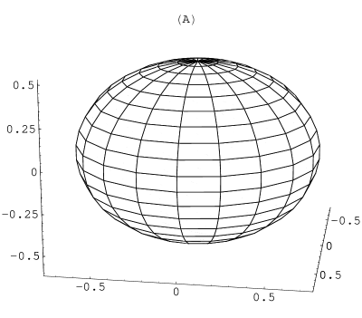
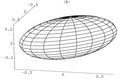
Figure 6: Shrinking of the full Bloch sphere into an oblate spheroid under evolution given by a Born-Markov type of dissipative interaction with $\gamma_{0}=0.6$ and temperature $T=5.0$. In (B), the $x$-$y$ axes are interchanged for convenience. (A) $r=\Phi=0$, $t=0.15$; (B) $r=0.4,\Phi=1.5$, $t=0.15$. Finite $\Phi$ is responsible for the tilt.

As in the case of the QND interaction, abstracting the effect of dissipative interaction into the Kraus representation allows us to subsume all the details of the system into a limited number of channel parameters $p_{1}(t)$, $\Phi$, $\alpha(t)$, $\mu(t)$ and $\nu(t)$. Any other dissipative system that can be described by a Lindblad-type master equation Eq. (19) will show a similar pattern in behavior.

To develop physical insight into the solution, we transform to the interaction picture, and for simplicity, set the squeezing parameters to zero. Then, the action of the operators (40), [which now represents a generalized amplitude channel] on an arbitrary qubit state is given in the Bloch vector representation by

$$\langle\vec{\sigma}(t)\rangle = (\langle\sigma_{1}(0)\rangle\sqrt{1-\lambda(t)},\langle\sigma_{2}(0)\rangle\sqrt{1-\lambda(t)},$$ (45)

$$\lambda(t)(1-2p)+\langle\sigma_{3}(0)\rangle(1-\lambda(t))),$$

where $p=(N_{\rm th}+1)/(2N_{\rm th}+1)$ and $\lambda(t=\infty)=1$. Thus, the Bloch sphere contracts towards the asymptotic mixed state $(0,0,1-2p)$ (Fig. 6(A)), characteristic of a generalized amplitude damping channel, with $T\geq 0$ and no squeezing. If $T=0$ case, then $p=1$, and the asymptotic state $(0,0,-1)$ is pure.

The Bloch vector picture allows us to interpret the results of Section 4.1. Eqs. (23), show that the Bloch vector for the states corresponding to $\theta_{0}=0,\pi$ move only along the $z$-axis of the Bloch sphere for zero as well as finite $T$. For the case $\theta_{0}=\pi$ and zero $T$, the Bloch vector remains stationary at $(0,0,-1)$, and hence GP vanishes. In the finite $T$ case, GP still vanishes, because the Bloch vector has the form $(0,0,-L(t))$, where the Bloch vector length $L(t)$ shrinks from 1 towards an interaction-dependent asymptotic value, which is zero for infinite temperature or finite otherwise. Since the Bloch vector shrinks strictly along its length, and thus subtends no finite angle at the center of the sphere, we find that GP vanishes at $\theta_{0}=\pi$, as expected (cf. Figs. 3).

On the other hand, even though the Bloch vector shrinks similarly along its length in the case $\theta_{0}=0$, we find that GP is non-vanishing in certain cases, in fact, in precisely those cases where the tip of the Bloch vector crosses the center of the Bloch sphere moving along the $\sigma_{3}$-axis. That is, they correspond to the situation where $\langle\sigma_{3}(t)\rangle$ changes sign from positive to negative during the period of one cycle. In these cases, the dependence of GP on the Bloch vector is too involved for us to interpret in terms of $L$ and the angle subtended by the Bloch vector, for some qualitative insight. Nevertheless this feature may be formally understood as follows. It can be observed from Eq. (24) that for sufficiently large $\gamma_{0}$, $\langle\sigma_{3}(t)\rangle$ changes sign at $t_{1}\equiv\log(2[N+1])/(\gamma_{0}[2N+1])$. Further, we note that $R$ vanishes for $\theta_{0}=0$ (as well as $\theta_{0}=\pi$).

It is convenient to recast Eq. (28) in the expanded form

$$\Phi_{\rm GP} = \tan^{-1}\left[\left(\sin(\chi(\tau)-\chi(0)+2\pi)\sin(\theta_{0}/2)\cos(\theta_{\tau}/2)\right)\right.$$ (46)

$$\div \{\cos(\chi(\tau)-\chi(0)+2\pi)\sin(\theta_{0}/2)\cos(\theta_{\tau}/2)$$

$$+ \left.\cos(\theta_{0}/2)\sin(\theta_{\tau}/2)\}\right]$$

$$- \int_{0}^{\tau}dt(\dot{\chi}(t)+\omega)\cos^{2}\left(\frac{\theta_{t}}{2}\right).$$

It can be seen that for the case $\theta_{0}=\pi$, $\cos(\theta_{t}/2)=1$ and, in particular, $\cos(\theta_{\tau}/2)=1$. Substituting these values in Eq. (46), it is seen that GP vanishes because the two terms in the RHS of Eq. (46) cancel each other. Next consider the case where $\theta_{0}=0$ but where $\gamma_{0}$ is sufficiently weak that $\tau\leq t_{1}$, i.e., $\langle\sigma_{3}(t)\rangle$ does not change sign during one cycle. In this case, from above it is seen that $\cos(\theta_{t}/2)=0$, and, in particular, $\cos(\theta_{\tau}/2)=0$, and thus the terms in the RHS of Eq. (46) vanish identically. But in the case of $\theta_{0}=0$ where $\tau>t_{1}$ ($\gamma_{0}$ being relatively stronger), $\cos(\theta_{t}/2)=0$ initially in the time interval $[0,t_{1}]$, and then switches to 1 in the interval $(t_{1},\tau]$. In particular, $\cos(\theta_{\tau}/2)=1$. Observe that if $\cos(\theta_{t}/2)=1$ throughout the interval $[0,\tau]$, the two terms in the RHS cancel each other. It follows that GP is non-vanishing because of an excess contributed by the first term, in the interval $[0,t_{1}]$.

Contraction produced by an increase in temperature tends to be less pronounced in the presence (than in the absence) of squeezing (Figs. 6). This is reflected in the slower variation of GP with respect to temperature, seen in Figs. 4(B) and 5(B) in relation to Figs. 4(A) and 5(A), respectively. As observed in Figs. 4 and 5, GP falls as a function of $T$, for sufficiently large $T$. This may quite generally be attributed to the reduction in $L$ and $\Omega$ caused by the contraction of Bloch vector as a result of interaction with the environment. The tilt of the contracted Bloch sphere in Fig. 6(B) is due to finite $\Phi$.

5 Conclusions

We have studied the combined influence of squeezing and temperature on the GP for a qubit interacting with a bath both in a non-dissipative as well as in a dissipative manner. In the former case, squeezing has a similar debilitating effect as temperature on GP. In contrast, in the latter case, squeezing can counteract the effect of temperature in some regimes. This makes squeezing potentially helpful for geometric quantum information processing and geometric computation. In particular, in the context of using engineered (e.g., squeezed) reservoirs to generate GP cor06 , it would be helpful to consider the effect of squeezing together with thermal effects rz06 ; lom06 .

In the non-dissipative (QND) case, we analyzed a number of open system models using two types of bath: the usual one of harmonic oscillators, and that of two-level systems. It was shown that for the case of weak $S{-}R$ coupling, the two kinds of baths can be mapped onto each other. GP was studied as a function of the initial polar angle $\theta_{0}$ of the Bloch sphere, temperature and squeezing (arising from the squeezed thermal bath). In the QND case, it was seen that increasing $\gamma_{0}$, temperature or squeezing tends to cause a similar departure from unitary behavior by suppressing GP.

However, in the dissipative case (with the environment modelled as a squeezed thermal bath in the weak Born-Markov RWA), we found that the dependence of GP on $\theta_{0}$, temperature and squeezing shows a greater complexity. Here, an interesting feature due to squeezing is that it can disrupt, over an interval, the otherwise monotonic behavior of GP as a function of $\theta_{0}$ (the humps seen in Figure 3(B)). More pronouncedly, the counteractive effect of squeezing on temperature is brought out by a comparison of Figures 4(A) with 4(B), and 5(A) with 5(B). Also, its effect on the Bloch sphere is to shrink it to an oblate spheroid, in contrast to a QND interaction, which produces a prolate spheroid. Thus, an interesting feature that emerges from our work is the contrast in the interplay between squeezing and thermal effects in non-dissipative and dissipative interactions. By interpreting the open quantum effects as noisy channels, we make the connection between geometric phase and quantum noise processes familiar from quantum information theory.

An added feature of our work is that we make a connection between the studied open system models and the phase damping and the newly introduced squeezed generalized amplitude damping srisub channels, noise processes which are important from a quantum information theory perspective. In particular, we give a detailed microscopic basis for these noisy channels. This allows us to study the effects of the formal noise processes on GP.

References

- (1) S. Pancharatnam, Proc. Indian Acad. Sci., Sect. A 44, 247 (1956).
- (2) M. V. Berry, Proc. R. Soc. London, Ser. A 392, 45 (1984).
- (3) B. Simon, Phys. Rev. Lett. 51, 2167 (1983).
- (4) Y. Aharonov and J. Anandan, Phys. Rev. Lett. 58, 1593 (1987).
- (5) J. Samuel and R. Bhandari, Phys. Rev. Lett. 60, 2339 (1988).
- (6) N. Mukunda and R. Simon, Ann. Phys. (N.Y.) 228, 205 (1993).
- (7) A. Uhlmann, Rep. Math. Phys. 24, 229 (1986); Ann. Phys. 46, 63 (1989); Lett. Math. Phys. 21, 229 (1991).
- (8) E. Sjöqvist, A. K. Pati, A. Ekert, et al., Phys. Rev. Lett. 85, 2845 (2000).
- (9) K. Singh, D. M. Tong, K. Basu, et al., Phys. Rev. A 67, 032106 (2003).
- (10) D. M. Tong, E. Sjöqvist, L. C. Kwek and C. H. Oh, Phys. Rev. Lett. 93, 080405 (2004).
- (11) Z. S. Wang, L. C. Kwek, C. H. Lai and C. H. Oh, Europhysics Lett. 74, 958 (2006);
- (12) Z. S. Wang, C. Wu, X.-L. Feng, L. C. Kwek et al., Phys. Rev. A 75, 024102 (2007).
- (13) M. -M. Duan, I. Cirac and P. Zoller, Science 292, 1695 (2001).
- (14) R. Balakrishna and M. Mehta, Eur. Phys. J. D 33 437, (2005).
- (15) G. Falci, R. Fazio, G. H. Palma, J. Siewert and V. Vedral, Nature (London) 407, 355 (2000).
- (16) J. A. Jones, V. Vedral, A. Ekert and G. Castagnoli, Nature (London) 403, 869 (2000).
- (17) Y. Nakamura, Yu. A. Pashkin and J. S. Tsai, Nature (London) 398, 786 (1999).
- (18) R. S. Whitney and Y. Gefen, Phys. Rev. Lett. 90, 190402 (2003); R. S. Whitney, Y. Makhlin, A. Shnirman and Y. Gefen, ibid., 94, 070407 (2005).
- (19) G. De Chiara, A. Lozinski and G. M. Palma, eprint quant-ph/0410183; to appear in Eur. Jl. of Physics D.
- (20) A. T. Rezakhani and P. Zanardi, Phys. Rev. A 73, 052117 (2006).
- (21) F. C. Lombardo, P. I. Villar, Phys. Rev. A 74, 042311 (2006); eprint quant-ph/0606036.
- (22) M. S. Sarandy and D. A. Lidar, Phys. Rev. A 73, 062101 (2006).
- (23) X. X. Yi, D. P. Liu and W. Wang, New Jl. of Physics 7, 222 (2005).
- (24) X. X. Yi, L. C. Wang and W. Wang, Phys. Rev. A 71, 044101 (2005).
- (25) X. X. Yi, D. M. Tong, L. C. Wang, et al., Phys. Rev. A 73, 052103 (2006).
- (26) T. A. B. Kennedy and D. F. Walls, Phys. Rev. A 37, 152 (1988).
- (27) M. S. Kim and V. Bužek, Phys. Rev. A 47, 610 (1993).
- (28) S. Banerjee and R. Ghosh, eprint quant-ph/0703054.
- (29) A. Carollo, G. M. Palma, A. Loziński et al., Phys. Rev. Lett. 96, 150403 (2006); eprint quant-ph/0507101.
- (30) K. Kraus, States, Effects and Operations (Springer-Verlag, Berlin, 1983).
- (31) M. Nielsen and I. Chuang, Quantum Computation and Quantum Information (Cambridge University Press, Cambridge, 2000).
- (32) R. Srikanth and S. Banerjee, eprint arXiv:0707.0059.
- (33) W. G. Unruh, Phys. Rev. A 51, 992 (1995).
- (34) G. M. Palma, K.-A. Suominen and A. K. Ekert, Proc. R. Soc. Lond. A 452, 567 (1996).
- (35) D. P. DiVincenzo, Phys. Rev. A 51, 1015 (1995).
- (36) C. M. Caves and B. L. Schumacher, Phys. Rev. A 31, 3068 (1985); B. L. Schumacher and C. M. Caves, Phys. Rev. A 31, 3093 (1985).
- (37) R. H. Dicke, Phys. Rev. 93, 99 (1954).
- (38) J. M. Radcliffe, J. Phys. A: Gen. Phys. 4, 313 (1971).
- (39) F. T. Arecchi, E. Courtens, R. Gilmore and H. Thomas, Phys. Rev. A 6, 2211 (1972).
- (40) J. Shao, M.-L. Ge and H. Cheng, Phys. Rev. E 53, 1243 (1996).
- (41) J. Shao and P. Hänggi, Phys. Rev. Lett. 81, 5710 (1998).
- (42) N. V. Prokof’ev and P. C. E. Stamp, Rep. Prog. Phys. 63, 669 (2000).
- (43) S. Banerjee and R. Srikanth, eprint quant-ph/0611161v2.
- (44) M. O. Scully and M. S. Zubairy, Quantum Optics (Cambridge University Press, Cambridge, 1997).
- (45) H.-P. Breuer and F. Petruccione, The Theory of Open Quantum Systems (Oxford University Press, 2002).
- (46) K.-P. Marzlin, S. Ghose and B. C. Sanders, Phys. Rev. Lett. 93, 260402 (2004).
- (47) R. Srikanth and S. Banerjee, Phys. Lett. A 367, 295 (2007); eprint quant-ph/0611263.