Coherent control of photon transmission :
slowing light in coupled resonator waveguide doped with $\Lambda$ Atoms

Abstract

In this paper, we propose and study a hybrid mechanism for coherent transmission of photons in the coupled resonator optical waveguide (CROW) by incorporating the electromagnetically induced transparency (EIT) effect into the controllable band gap structure of the CROW. Here, the configuration setup of system consists of a CROW with homogeneous couplings and the artificial atoms with $\Lambda$-type three levels doped in each cavity. The roles of three levels are completely considered based on a mean field approach where the collection of three-level atoms collectively behave as two-mode spin waves. We show that the dynamics of low excitations of atomic ensemble can be effectively described by an coupling boson model. The exactly solutions show that the light pulses can be stopped and stored coherently by adiabatically controlling the classical field.

I Introduction

Electromagnetically induced transparency (EIT) is a phenomenon that usually occurs for atomic ensemble as an active mechanism to slow down or stop laser pulse completely EIT97 ; EIT97-1 ; EIT01 ; EIT02 . Usually, the EIT effect happens in the so-called $\Lambda$-type atomic system, which contains two lower states with separate couplings to an excited state via two electromagnetic fields (probe and control light). When the absorption on both transitions is suppressed due to destructive interference between excitation pathways to the upper level, the medium becomes transparent with respect to the probe field.

Most recently, an EIT-like effect has been displayed in the experiment via all optical on-chip setups with the coupled resonator optical waveguide (CROW) Fanprl06 ; nat441 . The bare CROW for photons behaves as the tight-binding lattice with band structure for electrons, thus the CROW forms a new type photonic crystal. It was discovered that, by coupling each resonator in the CROW to an extra cavity, the resonate spectral line is shift and the band width is compressed, thus the propagating of light pulses is stopped and the information carried by light is stored Fanprl04 ; Fanprl05 ; Maol29 . The scheme of stopping, storing and releasing light is also theoretically proposed and analyzed for quantum-well Bragg structures which form a one-dimensional resonant photonic bandgap structures JOSAB1 .

Actually, with the help of modern nano-fabrication technology, the hybrid structure, i.e., an array of coupled cavities with doping artificial atoms can be implemented experimentally with a photonic crystal or other semiconductor systems. By making use of such hybrid system Bqp06159 ; Pqp06097 , Mott insulator and superfluid state can emerge in different phases of the polaritons formed by dressing the doping atoms with the gapped light field. Also the hybrid system of a two-dimensional array of coupled optical cavities in the photon-blockade regime will undergo a characteristic Mott insulator (excitations localized on each site) to superfluid (excitations delocalized across the lattice) quantum phase transition lqpt . Such a coplanar hybrid structure based on superconducting circuit, has been proposed by us scp06085 for the coherent control of microwave - photons propagating in a coupled superconducting transmission line resonator (CTLR) waveguide yale ; yale04 .

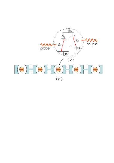
Figure 1: (Color on line) Illustrative configuration for controlling light propagation in a coupled resonators waveguide by doping atom systems: (a) A schematic of the coupled resonator optical waveguide (CROW) doped by three level systems. The CROW can be realized as a array of periodic defects in the photonic bandgap materials, or a waveguide with coupled superconducting transmission line resonators; (b). The doping three level atoms interacting with quantized probe light and the classical couple light. The artificial atoms can be realized as the quantum dot, or the charge and flux qubits.

By making use of the two time Green function approach, we studied the coherent control of photon transmission along the homogeneous CROW by doping two-level atomsFMHU . Usually, to realize the controllable and robust two-level system, a three-level atom is used to reduce an effective two level structure through the stimulated Raman mechanism, which is two photon process decoupling the two direct transitions to upper energy level in the case with large detuning. Then the induced coupling between two lower energy levels can be obtained by the adiabatic elimination of the upper energy level.

In this paper, we study the photon transmission in a homogeneous CROW controlled coherently by doped three-level $\Lambda$-type systems, where the upper energy level is not eliminated adiabatically. To consider the coherent roles of three energy levels directly, we use the mean field approach to deal with the collective excitations of all spatial distributed $\Lambda$ -type atoms as two independent bosonic modes of quasi-spin-waves Jin-GR . These quasi-spin-waves due to interacting with the cavity modes in CROW can change the photonic band structure of CROW so that the dispersion relation exhibits some exotic feature - a slow (and even zero velocity) light pulses can emerge by some appropriate coherent control of light-atom couplings.

This paper is organized as follow: In Sec. II, we describe our model - the homogeneous CROW with each cavity doping a $\Lambda$-type three-level atom. By the mean field approach in terms of spin wave excitations, in Sec.III, we derive down the effective Hamiltonian for the hybrid structure. In Sec. IV, we diagonalize the effective Hamiltonian to determine eigenfrequencies of this hybrid photon-atom system. The quasiparticles - polaritons are introduced to describe the excitations of this system. Then, in Sec. V, we discuss how the doping atoms modify the band structure of the CROW, and show how to store the information of incident pulse by adjusting the intensity of the control radiation in EIT. The absorption and dispersion of the atomic medium to the slow light pulses are studied in Sec. VI. We make our conclusion and give remarks shortly in sec. VII.

II Model setup and motivations

The hybrid system that we considered is shown in Fig.1. This system consists of $N$ single-mode cavities with homogeneous nearest-neighbor interaction, which form a one-dimensional array of cavities. Each single-mode cavity has the same resonance frequencies $\omega_{0}$. There are three practical systems to implement such array of cavities JOSAB2 : 1) a periodic array of coupled Fabry-Perot cavities; 2) the coupled microdisk or microring resonators; 3) the coupled defect modes in photonic crystals, where the bandgap cavities are formed when the periodicity of photonic crystal is broken periodically Stefa98 ; Bayin00 . The intercavity photon hopping is due to the evanescent coupling pathways between the cavities. In the coupled Fabry-Perot cavities and the microdisk or microring resonators, the doped system can be the natural atom. For photonic crystals, the photonic bandgap material is fabricated in diamond, the doping systems can be realized as some ion-implanted NV centers lqpt . Another promising candidate for electromagnetically controlled quantum device is based on superconducting circuit scp06085 , where the CROW is realized by the superconducting waveguide with coupled transmission line resonators yale ; yale04 , while the doping systems are implemented by the biased Cooper pair boxes (CPBs) (or called charge qubits), or the current biased flux qubits.

Generally, we use $a_{j}^{{\dagger}}$ ($a_{j}$) to denote its creation (annihilation) operator of the $j$th cavity. In each cavity, the two lower levels $\left|b\right\rangle$ and $|c\rangle$ are excited to the upper level $\left|f\right\rangle$ by the quantized field and the coupling field respectively. The energy level spacing between the upper level $\left|f\right\rangle$ and the ground state $\left|b\right\rangle$ is denoted by $\omega_{fb}=\omega_{f}-\omega_{b}$. This two-level atomic transition couples to quantized radiation modes of the waveguide cavities with coupling constant $g_{1}$. The energy difference between the upper level $\left|f\right\rangle$ and the metastable lower state $\left|c\right\rangle$ is denoted by $\omega_{fc}=\omega_{f}-\omega_{c}$. The atomic transition from $\left|f\right\rangle$ to $\left|c\right\rangle$ is driven homogeneously by an classical field of frequency $\Omega$ with coupling constant $g_{2}$.

Let $J$ be the nearest-neighbor evanescent coupling constant of intercavity. The model Hamiltonian $H=H_{C}+H_{A}+H_{AC}$ consists of three parts, the cavity part with intercavity photon hoppings,

$$H_{C}=\sum_{j}^{N}\omega_{0}a_{j}^{{\dagger}}a_{j}+J\sum_{j=1}^{N}a_{j}^{{\dagger}}a_{j+1}+h.c.,$$ (1)

the free atom part,

$$H_{A}=\sum_{j}^{N}\left(\omega_{f}\sigma_{ff}^{j}+\omega_{b}\sigma_{bb}^{j}+\omega_{c}\sigma_{cc}^{j}\right),$$ (2)

and the localized photon-atom interaction part

$$H_{AC}=\sum_{j}^{N}\left(g_{1}\sigma_{fb}^{j}a_{j}+g_{2}e^{-i\Omega t}\sigma_{fc}^{j}+h.c.\right)$$ (3)

Here, the quasi-spin operators $\sigma_{\alpha\beta}^{j}=|\alpha\rangle_{j}\langle\beta|$ ($\alpha,\beta=f,b,c$) for $\alpha\neq\beta$ describe the atomic transitions among the energy levels of $|f\rangle$, $|b\rangle$ and $|c\rangle$. In practical experiments, coupling constants $g_{i}$ and $J$ depend on the positions of atoms. In this paper, we take uniform $g$ and $J$ for simplicity. Actually, a small difference of couplings is unavoidable in the practical implementation of the present setup, but there should been no principle difficulty in modern fabrication technique to achieve quasi uniform coupling sunprb71 . Theoretically, the small fluctuations of coupling constants are innocuous and do not change the results of this paper qualitatively.

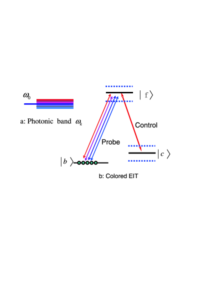
Figure 2: (Color on line) Electromagnetically induced transparency (EIT) effect in the coupled resonator optical waveguide (CROW) with photonic band structure: The problem is equivalent to that a multi-mode optical pulse with different color component couples between two energy levels near-resonantly. The strong light split the bare energy levels. The EIT phenomenon emerges when the band structure can match these split. This mechanism can well controls light propagation in the CROW by doping a three-level system.

To illustrate our motivation using this complex hybrid structure, we may recall the fundamental principle for the EIT phenomenon briefly. Usually, a absorption region occurs to a weak probe light when it passes through a medium, but in the presence of the control light, a transparency “window” appears in the probe absorption spectrum. Here the probe light is not of single color since the photon propagating in the CROW has a photonic band. To consider whether or not EIT phenomenon emerges in this band-gap structure, we should match the photonic band structure with the splits of the energy level spacing between $|f\rangle$ and $|c\rangle$ (see the Fig.2).

As for this hybrid structure with EIT effect, it is well known that, among varieties of theoretical treatments of EIT, an approach for EIT is the “dressed state” picture, wherein the Hamiltonian of the system plus the light field is diagonalized firstly to give rise to a Autler-Townes like splitting Autler in the strong coupling limit with the control field. Then the Fano like interference Fano124 between the dressed states results in EIT. Between the doublet peaks of the absorption line, a transparency window emerges as the quantum probability amplitudes for transitions to the two lower states interference. In the CROW, the emitted and absorbed photons can also be constrained by the photonic band structure. Here, the single and two photon resonances in EIT for a given Autler-Townes like splitting should be re-considered to match the band structure of the CROW. Particularly, we need to generalize the polariton approach to describe the stopped and stored light schemes. Here, the photons of the probe beam only within the photonic band can be coherently “transformed” into “dark state polaritons” , which are the dressed excitations of atom ensemble.

III Collective Excitations with Electromagnetically Induced Transparency Effect

In order to study the novel EIT effect in the CROW, we use the mean field approach that we developed for the collective excitation of an atomic ensemble with a ordered initial state sunprl91 . This approach for EIT can be understood as a fully-quantum theory, which not only gives these results about slow light propagation that can be given by semi-classical approach, but also emphasizes the quantum states of photon and the atomic collective excitations - quasi-spin waves, which are crucial for quantum information processing, such as quantum memory or storage

Let $\ell$ be the distance between the nearest-neighbor cavities. The Fourier transformation

$$A_{k} = \frac{1}{\sqrt{N}}\sum_{j}\sigma_{bf}^{j}\exp(ik\ell j)$$ (4)

$$C_{k} = \frac{1}{\sqrt{N}}\sum_{j}\sigma_{bc}^{j}\exp(ik\ell j)$$ (5)

and its conjugate $A_{k}=(A_{k}^{{\dagger}})^{{\dagger}}$, $C_{k}=(C_{k}^{{\dagger}})^{{\dagger}}$  define the boson-like operators to describe the collective excitation from $|b\rangle$ to $|f\rangle$ and from $|b\rangle$ to $|c\rangle$ respectively. In the large $N$ limit, and under the low excitation condition that there are only a few atoms occupying $|f\rangle$ or $|c\rangle$, the quasi-spin-wave excitations behave as bosons since they satisfy the bosonic commutation relations

$$[A_{k},A_{k}^{{\dagger}}] = 1,[C_{k},C_{k}^{{\dagger}}]=1.$$

$$[A_{k},C_{k}] = 0,$$ (6)

$$[A_{k},C_{k}^{{\dagger}}] = -\frac{T_{-}}{N}\rightarrow 0$$

Thus these quasi-spin-wave low excitations are independent of each other. Here, the collective operators

$$T_{-} = \sum_{j}^{N}\sigma_{cf}^{j},T_{+}=\left(T_{-}\right)^{{\dagger}}$$ (7)

$$T_{3} = \frac{1}{2}\sum_{j}\left(\sigma_{ff}^{j}-\sigma_{cc}^{j}\right)$$ (8)

generates the $SU(2)$ algebra.

In a rotating frame with respect to the 0’th order Hamiltonian

$$H_{0}=\sum_{j}^{N}(\omega_{0}a_{j}^{{\dagger}}a_{j}+\omega_{f}^{\prime}\sigma_{ff}^{j}+\omega_{b}\sigma_{bb}^{j}+\omega_{c}\sigma_{cc}^{j})$$

we achieve the coupling boson mode with the model Hamiltonian $H=\sum_{k}H_{k}:$

$$H_{k} = \delta_{2}A_{k}^{{\dagger}}A_{k}+\Omega_{k}a_{k}^{{\dagger}}a_{k}$$ (9)

$$+g_{1}A_{k}^{{\dagger}}a_{k}+g_{2}A_{k}^{{\dagger}}C_{k}+h.c.$$

where we have used the Fourier transformation

$$\hat{a}_{k}=\frac{1}{\sqrt{N}}\sum_{j}\hat{a}_{j}\exp(ik\ell j).$$

Here, $\omega_{f}^{\prime}=\omega_{f}-\delta_{1}$, $\delta_{1}=\omega_{fb}-\omega_{0}$ is detuning between the quantized mode and the transition frequency $\omega_{fb}$, and $\delta_{2}=\omega_{fc}-\Omega$ is detuning between the classical field and the transition frequency $\omega_{fc}$. The original band structure is characterized by the dispersion relation

$$\Omega_{k}=\delta_{2}-\delta_{1}+2J\cos\left(k\ell\right).$$ (10)

Obviously the photonic band is centered at $k=\pi/(2\ell)$.

To enhance the coupling strength between the probe field and atoms, we can dope more, say $N_{A}$, identical noninteractive three-level $\Lambda$-type atoms in each cavity. In this case, the system Hamiltonian is changed into

$$H=H_{C}+\sum_{j}(H_{A}^{j}+H_{CA}^{j})$$

with

$$H_{A}^{j}=\omega_{f}s_{ff}^{j}+\omega_{b}s_{bb}^{j}+\omega_{c}s_{cc}^{j}\text{,}$$ (11)

$$H_{CA}^{j}=g_{1}s_{fb}^{j}a_{j}+g_{2}e^{-i\Omega t}s_{fc}^{j}+\text{H.c.,}$$ (12)

where, in each cavity,

$$s_{\alpha\beta}^{j}=\sum_{l}\sigma_{\alpha\beta j}^{l}$$ (13)

denote the collective dipole between $|\alpha\rangle$ and $|\beta\rangle$ for $\alpha\neq\beta$.

For each cavity, the collective effect of doped three-level atoms can be described by quasi-spin-wave boson operators

$$A_{j}=\frac{s_{bf}^{j}}{\sqrt{N_{A}}},C_{j}=\frac{s_{bc}^{j}}{\sqrt{N_{A}}},$$ (14)

which create two collective states $|1_{c}\rangle_{j}=C_{j}^{{\dagger}}|\nu\rangle$ and $|1_{f}\rangle_{j}=A_{j}^{{\dagger}}|\nu\rangle$ with one quasi-particle excitations. Here $|\nu\rangle=|b_{1},b_{2},\ldots,b_{N_{A}}\rangle$ is the collective ground state with all $N_{A}$ atoms staying in the ground state $|b\rangle$. In low excitation and large $N_{A}$ limit, the two quasi-spin-wave excitations behave as two bosonssunprl91 , and they satisfy the bosonic commutation relations

$$[A_{j},A_{j}^{{\dagger}}]=1,[C_{j},C_{j}^{{\dagger}}]=1,$$ (15)

and $[A_{j},C_{j}]=0$. The commutation relations between $A_{j}$ and $C_{j}$ means that, in each cavity, the two quasi-spin-wave generated by $N_{A}$ three-level $\Lambda$-type atoms are independent of each other.

In the interaction picture with respect to

$$H_{0}=\omega_{0}\sum_{j}^{N}a_{j}^{{\dagger}}a_{j}+\sum_{j}^{N}\left[\omega_{f}^{\prime}s_{ff}^{j}+\omega_{b}s_{bb}^{j}+\omega_{c}s_{cc}^{j}\right],$$

and by the Fourier transformations

$$F_{k}=\sum_{j}\frac{F_{j}}{\sqrt{N_{A}}}e^{ik\ell j}$$ (16)

for $F=a,A$ and $C$ et al, the interaction Hamiltonian reads as $V=\sum_{k}V_{k}$:

$$V_{k} = \epsilon_{k}a_{k}^{{\dagger}}a_{k}+\delta_{2}A_{k}^{{\dagger}}A_{k}$$ (17)

$$+G_{1}A_{k}^{{\dagger}}a_{k}+g_{2}A_{k}^{{\dagger}}C_{k}+h.c.$$

where

$$\epsilon_{k}=2J\cos\left(k\ell\right)+\delta_{2}-\delta_{1}$$ (18)

is the dispersion relation of CROW. Here, the effective photonic band-spin wave coupling $G_{1}=g_{1}\sqrt{N_{A}}$ is $\sqrt{N_{A}}$ times enhancement of $g_{1}$ and thus result in a strong coupling.

We also notice that the $SU(2)$ algebra defined by the quasi-spin operators $T_{-},T_{+}$ and $T_{3}$ in the coordinate space can also be realized in the momentum space through the Fourier transformations as

$$(T_{-})_{k} = A_{k}^{{\dagger}}C_{k},(T_{+})_{k}=C_{k}^{{\dagger}}A_{k}$$

$$(T_{3})_{k} = \frac{1}{2}(C_{k}^{{\dagger}}C_{k}-A_{k}^{{\dagger}}A_{k})$$ (19)

This means the interaction Hamiltonian possesses a intrinsic dynamic symmetry described by a large algebra containing $SU(2)$ as subalgebra. Technologically this observation will help us to diagonalize the Hamiltonian Eq.(17) as follows.

IV Dressed collective states: polaritons

In each cavity the strong couplings will coherently mix the photon and the artificial atoms to form dressed states. The collective effect of these dressed states can make the collective excitations, which behave as bosons (called polaritons)  in the low excitation limit. Mathematically we write the boson operator $a_{k}$, $A_{k}$ and $C_{k}$ as an operator-valued vector

$$\vec{b}_{k}=\left(\begin{array}[]{c}a_{k}\\ A_{k}\\ C_{k}\end{array}\right).$$

In terms of those operator-valued vectors {$\vec{b}_{k}$}, the interaction Hamiltonian $V_{k}$ can be re-written as

$$V_{k}=\vec{b}_{k}^{{\dagger}}M\vec{b}_{k},$$

where

$$M=\left[\begin{array}[]{ccc}\epsilon_{k}&G_{1}&0\\ G_{1}&\delta_{2}&g_{2}\\ 0&g_{2}&0\end{array}\right].$$

Now we solve eigenvalue problem of the matrix $M$. Then $V_{k}$ can be diagonalized to construct the polariton operators, which is described by the linear combination of the quantized electromagnetic field operators and atomic collective excitation operator of quasi-spin waves. The three real eigenvalues of $M$

$$\lambda_{k}^{[1]} = \beta_{+}^{[k]}+\beta_{-}^{[k]}+\frac{1}{3}(\epsilon_{k}+\delta_{2})$$

$$\lambda_{k}^{[2]} = \varkappa\beta_{+}^{[k]}+\varkappa^{2}\beta_{-}^{[k]}+\frac{1}{3}(\epsilon_{k}+\delta_{2})$$ (20)

$$\lambda_{k}^{[3]} = \varkappa^{2}\beta_{+}^{[k]}+\varkappa\beta_{-}^{[k]}+\frac{1}{3}(\epsilon_{k}+\delta_{2})$$

are written in terms of $\varkappa=(-1+i\sqrt{3})/2$ and

$$\beta_{\pm}^{[k]}=\sqrt[3]{-\frac{q}{2}\pm\sqrt{\left(\frac{q}{2}\right)^{2}+\left(\frac{p}{3}\right)^{3}},}$$

$$p = -\frac{1}{3}\epsilon_{k}^{2}+\frac{1}{3}\delta_{2}\epsilon_{k}-G_{1}^{2}-g_{2}^{2}-\frac{1}{3}\delta_{2}^{2},$$

$$q = \frac{1}{27}\left[3\delta_{2}\epsilon_{k}^{2}-2\epsilon_{k}^{3}+\left(18g_{2}^{2}-9G_{1}^{2}+3\delta_{2}^{2}\right)\epsilon_{k}\right.$$

$$\left.-2\delta_{2}^{3}-9G_{1}^{2}\delta_{2}-9g_{2}^{2}\delta_{2}\right],$$

For a nonzero eigenvalue $\lambda_{k}^{[i]}$, the polariton operators can be defined as

$$P_{k}^{[i]}=\frac{1}{r_{i}}\left[\frac{G_{1}}{\lambda_{k}^{[i]}-\epsilon_{k}}a_{k}+A_{k}+\frac{g_{2}}{\lambda_{k}^{[i]}}C_{k}\right],$$ (21)

where

$$r_{i}=\sqrt{\frac{|G_{1}|^{2}}{|\lambda_{k}^{[i]}-\epsilon_{k}|^{2}}+1+\frac{|g_{2}|^{2}}{|\lambda_{k}^{[i]}|^{2}}}.$$ (22)

When the detunings approximately satisfy the resonance transition condition so that $\epsilon_{k}=0$ for some $k,$ the dark-state polariton can be constructed as an eigenstate with vanishing eigenvalue. For concreteness, we first consider the case with the detuning $\delta_{2}=\delta_{1}=0$, which means that the probe light and the classical field are resonant with the $\Lambda$-type atoms in each cavity. The polariton operators at the band center $k=k_{0}=\pi/(2\ell)$ can be constructed as

$$P_{k_{0}}^{[1]} = \frac{1}{\sqrt{2}}(A_{k_{0}}-B_{k_{0}})$$ (23a)

$$P_{k_{0}}^{[2]} = a_{k_{0}}\cos\theta-C_{k_{0}}\sin\theta$$ (23b)

$$P_{k_{0}}^{[3]} = \frac{1}{\sqrt{2}}(A_{k_{0}}+B_{k_{0}})$$ (23c)

with $$\tan\theta=G_{1}/g_{2}$$, and

$$B_{k_{0}}=a_{k_{0}}\cos\theta+C_{k_{0}}\sin\theta.$$ (24)

Here, $P_{k_{0}}^{[2]}$ is the dark-state polariton (DSP), which traps the electromagnetic radiation from the excited state due to quantum interference cancelling; $B_{k_{0}}$ is called the bright-state polaritonsunprl91 .

For another case, we assume that, in each cavity, the frequency of the probe light $\omega_{0}$ has a nonzero detuning from the transition frequency $\omega_{ab}$, i.e. $\delta_{1}=\Delta\neq 0$. By adjusting the frequency of the classical field, $\delta_{2}=\Delta$ can be realized, and then the condition $\epsilon_{k}=0$ is satisfied at the band center. So the dark-state polariton exists. With the polariton operators

$$Q_{k_{0}}^{[1]} = \xi\left[G_{1}a_{k_{0}}+\frac{\Delta-\alpha}{2}A_{k_{0}}+g_{2}C_{k_{0}}\right],$$ (25a)

$$Q_{k_{0}}^{[2]} = a_{k_{0}}\cos\theta-C_{k_{0}}\sin\theta,$$ (25b)

$$Q_{k_{0}}^{[3]} = \xi\left[G_{1}a_{k_{0}}+\frac{\Delta+\alpha}{2}A_{k_{0}}+g_{2}C_{k_{0}}\right],$$ (25c)

for

$$\xi=\sqrt{2/\left(\alpha-\Delta\right)\alpha},$$

the interaction Hamiltonian $V_{k_{0}}$ is diagonalized. Here,

$$\alpha=\sqrt{\Delta^{2}+4G_{1}^{2}+4g_{2}^{2}}.$$ (26)

the DSP $Q_{k_{0}}^{[2]}$ is the specific light-matter dressed states, which particularly appears in EIT.

Actually, for a probe light with nonzero detuning $\delta_{1}$ and small band around $k=k_{1}$ ($k_{1}\neq k_{0}$), by adjusting the detuning $\delta_{2}$ to satisfy $\epsilon_{k_{1}}=0$, at the model $k=k_{1}$, we can also construct the polariton operators similar to those of Eq. (25) with $\delta_{2}$ replacing $\Delta$ and $k_{1}$ replacing $k_{0}$.

V
Band structure of polaritons

From the above discussion, it can be observed that the spectra of the hybrid system consists of three bands, and there exists gaps among these three bands for a non-vanishing $G_{1}$ and $g_{2}$. Since the number of total excitations

$$N_{k}=a_{k}^{{\dagger}}a_{k}+A_{k}^{{\dagger}}A_{k}+C_{k}^{{\dagger}}C_{k}$$ (27)

commutes with $V_{k}$, the number of excitation $N_{k}$ is conserved , while the numbers $a_{k}^{{\dagger}}a_{k}$, $A_{k}^{{\dagger}}A_{k}$ and $C_{k}^{{\dagger}}C_{k}$ of different type excitations are mutually convertible by adjusting some parameters. In Fig.3 we plot the eigenfrequencies as a function of the wave vector $k$ in the one excitation subspace.

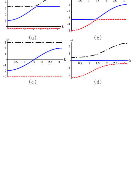
Figure 3: (Color on line) The band structure at the first excitation space. Here the eigenfrequency is plotted as a function of the wave vector $k$. We have set $J=-1$. The other parameter are set as follow, $\delta_{1}=0$, (a)$\delta_{2}=3|J|$, $G_{1}=0.1J$, $g_{2}=1.0|J|$, ( b)$\delta_{2}=-3|J|$, $G_{1}=0.1J$, $g_{2}=1.0|J|$. (c)$\delta_{2}=0$, $G_{1}=0.1|J|$, $g_{2}=3|J|$, (d)$\delta_{2}=0$, $G_{1}=|J|$, $g_{2}=0.1|J|$. The wave vector $k$ is in unit of $1/\ell$.

It can be seen from Figs. 3(a) and (b) that the bandwidth can be tuned by adjusting the detuning $\delta_{2}$ and the coupling strength $g_{2}$. For a fixed coupling strength $g_{2}$, when $\delta_{2}\ll-|g_{2}|$, the lowest band (the red dash line) has a large bandwidth, which ensures to accommodate the bandwidth of entire pulse; when $\delta_{2}\gg|g_{2}|$, the bandwidth of the lowest band $W_{0}\approx 0$. Hence for a light pulse that is a superposition of many $k$-states, its distribution in the $k$ -space can be entirely contained in the photonic band of the CROW by setting $\delta_{2}\ll-|g_{2}|$. By adiabatically tuning the detuning from $\delta_{2}\ll-|g_{2}|$ to $\delta_{2}\gg|g_{2}|$, the light pulse can be stopped. Such kind approach to stoping light with all-optical process has been investigated theoretically by numerical simulations Fanprl04 ; Fanprl05 ; Maol29 and a similar all-optical scheme has already been realized in a recent experiment Fanprl06 .

When the light pulse enters the medium, photons and atoms combine to form excitations known as polaritons. Because the spin wave propagates together with the light pulse inside the medium, the group velocity of light pulse is reduced by a large order of magnitude. Thus by analyzing the contribution of photons to the polaritons, it can be well understood that how the group velocity of probe field is stopped and revived. For the sake of simplify, firstly, we focus on the polaritons at the band center and consider the situation with the resonance transition. The operators of polaritons are the linear combination of that of photons and atoms with the following form

$$P_{k_{0}}^{[1]} = \frac{1}{\sqrt{2}}(A_{k_{0}}-a_{k_{0}}\cos\theta-C_{k_{0}}\sin\theta)$$ (28a)

$$P_{k_{0}}^{[2]} = a_{k_{0}}\cos\theta-C_{k_{0}}\sin\theta$$ (28b)

$$P_{k_{0}}^{[3]} = \frac{1}{\sqrt{2}}(A_{k_{0}}+a_{k_{0}}\cos\theta+C_{k_{0}}\sin\theta)$$ (28c)

where

$$\cos\theta = \frac{g_{2}}{\sqrt{g_{2}^{2}+G_{1}^{2}}}$$ (29)

$$\sin\theta = \frac{G_{1}}{\sqrt{g_{2}^{2}+G_{1}^{2}}}.$$ (30)

The contribution of photons to dark polaritons can be explicitly analyzed. It can be obtained that the dark polariton appears like photons with probability approximately to one when $g_{2}\gg G_{1}$, that is, $P_{k_{0}}^{[2]}\approx a_{k_{0}}$. Thus if we initial set $g_{2}\gg G_{1}$, this means the middle band can accommodate many component of the input pulse. It is easy to find that when $g_{2}\ll G_{1}$, the contribution of photons in the polariton becomes purely atomic, that is, $P_{k_{0}}^{[2]}\approx C_{k_{0}}$. Thus when the pulse is completely in the system, the adiabatical performance changes the dark polariton from photons to atoms and reverse. The similar situation can be found at the second band under the two photon resonance from Eq. (25).

In order to give a general argument, we plot the coefficients before $a_{k}$, $A_{k}$ and $C_{k}$ in the polaritons as functions of the momentum index $k$ respectively in Fig.4. For the convenience of expression, we denote $d_{jk}^{[i]}$ ($j=1,2,3$) as the coefficients before the operators $a_{k}$, $A_{k}$ and $C_{k}$ for different eigenvalues $i=1,2,3$ respectively. From Eq. (21), the expression of $d_{jk}^{[i]}$ can be obtained

$$d_{1k}^{[i]} = \frac{1}{r_{i}}\frac{G_{1}}{\lambda_{k}^{[i]}-\epsilon_{k}},$$

$$d_{2k}^{[i]} = \frac{1}{r_{i}},$$ (31)

$$d_{3k}^{[i]} = \frac{1}{r_{i}}\frac{g_{2}}{\lambda_{k}^{[i]}}.$$

In each figure,

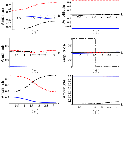
Figure 4: (Color on line) the contribution of photons and two spin waves in the polaritons $d_{jk}$ as functions of $k$ for the first eigenfrequency $\lambda_{k}^{[1]}$ (a) and (b), the second eigenfrequency $\lambda_{k}^{[2]}$ (c) and (d), the third eigenfrequency $\lambda_{k}^{[3]}$ (e) and (f). $\delta_{1}=\delta_{2}=0$, $J=-1$ . For (a), (c) and (e), we set $G_{1}=|J|$ and $g_{2}=0.1|J|$; For (b), (d) and (f), we set $G_{1}=0.1|J|$ and $g_{2}=3|J|$. The wave vector $k$ is in unit of $1/\ell$

the red dash line represents the magnitude $d_{2k}^{[i]}$ of spin waves generated by the atomic transition between $|b\rangle$ and $|f\rangle$; the blue solid line denotes the amplitude $d_{3k}^{[i]}$ of spin waves between $|b\rangle$ and $|c\rangle$; the black dash-dot line describes the magnitude $d_{1k}^{[i]}$ of photonic component. It can be observed that for the incident pulse with momentum distribution around $k=\pi/(2\ell)$, photons make a large contribution to the polaritons at $G_{1}\gg g_{2}$ than at the condition $G_{1}\ll g_{2}$. The contribution of photons in the polariton of the second band, shown in Fig. 4(c) and (d), is modified completely by the coupling strength of light and matter: spin waves $C_{k}$ take large proportions when $G_{1}\gg g_{2}$ and photons $a_{k}$ have large contributions when $G_{1}\ll g_{2}$. Hence the second band can be used to convert the quantum information originally carried by photons into long-lived spin states of atoms.

The characteristic of our hybrid system is that the “dark state”can be realized in a straightforward way. This gives rise to quasi-particles - the dark polariton, which reflects the crucial idea of the EIT - the coherent population trapping for the quantized probe field. Actually, a DSP is an atomic collective excitation (quasi-spin wave) dressed by the quantized probe light. This point can be seen directly from Eq.(25b). The contributions of light or atoms in DSP can be varied by adapting the amplitude of the classical field, which has been discussed in the last paragraph. Thus, in our hybrid system, the DSP offers a possible control scheme for slowing light. This accessible scheme can be observed from the change of bandwidth. In Fig. 3(c) and (d), we plot the eigenfrequency as a function of the wave vector $k$ in the first excitation space for a given $\delta_{2}$. It shows that, when $g_{2}\gg G_{1}$, the bandwidth of the middle band (the blue solid line) has a large bandwidth; when $g_{2}\ll G_{1}$, the bandwidth of the middle are approximately to zero; The couplings also make the center of bands away from $\omega_{0}$, $\omega_{ab}$ and $\omega_{cb}$ respectively. This fact means that by tuning the coupling strength from $g_{2}\gg G_{1}$ to $g_{2}\ll G_{1}$ adiabatically, we can stop the input light pulse and then re-emit it. Thus via selecting a classical field with a suitable frequency, the quantum state of an input pulse can be converted into the doped three-level atoms simply by switching off the driving field, and then by turning on the driving field, the stored information can be retrieved.

To give a concrete example, we consider the resonant transition with $\delta_{1}=\delta_{2}=0$. In this case, the corresponding group velocities at each band center are

$$v_{g}^{1}\left[k_{0}\right] = \frac{G_{1}^{2}}{G_{1}^{2}+g_{2}^{2}}J\ell,$$ (32)

$$v_{g}^{2}\left[k_{0}\right] = \frac{2g_{2}^{2}}{G_{1}^{2}+g_{2}^{2}}J\ell,$$ (33)

$$v_{g}^{3}\left[k_{0}\right] = \frac{G_{1}^{2}}{G_{1}^{2}+g_{2}^{2}}J\ell,$$ (34)

It can be seen that, at the band center, when $g_{2}\gg G_{1}$, the lowest band (the red dash line in Fig.3(c) and (d)) and the highest band (the black dash-dot line in Fig. 3(c) and (d)) exhibit zero group velocity and zero bandwidth, but the middle band (the blue solid one in Fig.3(c) and (d)) exhibits a large group velocity and a large bandwidth; in reverse, when $g_{2}\ll G_{1}$, the middle band exhibits zero group velocity and vanishing bandwidth, but the lowest band and the highest band exhibit large group velocities and large bandwidths. Hence in this system, focusing on the middle band, a light pulse can be stopped by the following process: Initially setting $g_{2}\gg G_{1}$, the middle band accommodates the entire pulse. After the pulse is completely in this system, we vary the coupling strength until $g_{2}\ll G_{1}$ adiabatically. The lowest band also can be used to stop light by tuning $g_{2}$ from $g_{2}\ll G_{1}$ to $g_{2}\gg G_{1}$.

Finally, we give some estimation about the group velocity according to the realistic parameters, which are taken for the array of coupled toroidal microcavitiesPqp06097 ; Spipra05 . The distance $\ell$ between the microcavities is $15.69\mu m$ Fanprl06 , and the evanescent coupling between the cavities $J=1.1\times 10^{7}s^{-1}$. Within each cavity, the coupling strength between the atom and the quantum field $g_{1}=2.5\times 10^{9}s^{-1}$, Rabi frequency $g_{2}=7.9\times 10^{10}s^{-1}$. When $N=10,000$ atoms are contained in each cavity, the group velocity of light at the second band center is estimated $31m/s$.

VI Susceptibility analysis for light propagation in the doped CROW

When a light beam incidents on an optically active medium, the medium will give a response to the control light. Usually, the index of refraction can reach high values near a transition resonance, but the high dispersion always accompanies with a high absorption in the resonance point. In EIT, the resonant transition or the two photon resonance renders a medium transparent over a narrow spectral range within the absorption line. Also in this transparent window, the rapidly varying dispersion is created, which leads to very slow group velocity and zero group-velocity. In this section, we will investigate the dispersion and the absorption property of the gapped light in our hybrid system. We use the dynamic algebraic method developed for the atomic ensemble based quantum memory with EIT sunprl91 ; sunpra69 .

We begin with the Hamiltonian (17) in the $k$-space representation. When the atomic decay is considered, we write down the Heisenberg equations of operators $a_{k}$, $A_{k}$ and $C_{k}$ for each mode $k$

$$\partial_{t}a_{k} = -(\gamma+i\epsilon_{k})a_{k}-iG_{1}A_{k},$$ (35)

$$\partial_{t}A_{k} = -\left(\gamma_{A}+i\delta_{2}\right)A_{k}-iG_{1}a_{k}-ig_{2}C_{k},$$ (36)

$$\partial_{t}C_{k} = -\gamma_{C}C_{k}-ig_{2}A_{k}$$ (37)

where we have phenomenologically introduced the damping rate of cavity $\gamma$, and the decay rate $\gamma_{A}$, $\gamma_{C}$ of the energy levels $|f\rangle$ and $|c\rangle$ of the three-level system respectively. We also assume that

$$\gamma_{A}\gg\gamma_{C}\gg\gamma.$$

To find the steady-state solution for the above motion equations, it is convenient to remove the fast varying part of the light field and the atomic collective excitations by making a transformation

$$F_{k}=\tilde{F}_{k}e^{-i\epsilon_{k}t}$$ (38)

for $F_{k}=a_{k}$, $A_{k}$ and $C_{k}$. For the convenience of notation, we drop the tilde, and then the above Heisenberg equations become

$$\partial_{t}C_{k} = \left(i\epsilon_{k}-\gamma_{C}\right)C_{k}-ig_{2}A_{k},$$ (39)

$$\partial_{t}A_{k} = \left[i\left(\omega_{k}-\delta_{1}\right)-\gamma_{A}\right]A_{k}-iG_{1}a_{k}-ig_{2}C_{k},$$

where $\omega_{k}=2J\cos\left(k\ell\right)$.

The electric field of the quantized probe light with $k$-space representation

$$E_{k}(t)=\sqrt{\frac{\omega_{0}}{2V\varepsilon_{0}}}a_{k}e^{-i\epsilon_{k}t}+h.c.$$ (40)

results in a linear response of medium, which is described by the polarization

$$\left\langle P_{k}\right\rangle=\left\langle p_{k}\right\rangle\exp(-i\epsilon_{k})+h.c.$$

Here,

$$\left\langle p_{k}\right\rangle=\frac{\mu}{V}\sqrt{N_{A}}\left\langle A_{k}\right\rangle$$ (41)

is a slowly varying complex polarization determined by the population distribution on $|f\rangle$ and $|c\rangle$; $\mu$ denotes the dipole moment between $|f\rangle$ and $|c\rangle$, and $V$ is the effective mode volumebqoptics . It is also related to the susceptibility $\chi_{k}$ of the $k$-space by

$$\left\langle p_{k}\right\rangle=\epsilon_{0}\chi_{k}\sqrt{\frac{\omega_{0}}{2V\varepsilon_{0}}}\left\langle a_{k}\right\rangle.$$ (42)

The real part $\chi_{k}^{r}$ and imaginary part $\chi_{k}^{i}$ of the susceptibility correspond to the dispersion and absorption respectively.

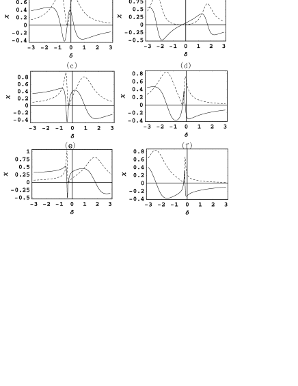
Figure 5: Real (solid) and imaginary (dotted) parts of the linear susceptibility as a function of normalized detuning $\delta$ at $k=\pi/4$. The parameters are set as $G_{1}=1$, $J=0.2$, $\ell=1$. (a) $g_{2}=0.5$, $\delta_{2}=0$; (b) $g_{2}=2$, $\delta_{2}=0$; (c)$g_{2}=0.5$, $\delta_{2}=1$; (d)$g_{2}=0.5$, $\delta_{2}=-1$; (e)$g_{2}=0.5$, $\delta_{2}=2$; (f)$g_{2}=0.5$, $\delta_{2}=-2$. $\delta$ is in units of $\gamma_{A}=1$

In order to calculate the susceptibility, we first find the steady-state solution by letting $\partial_{t}A_{k}=0$ and $\partial_{t}C_{k}=0$ in the Eq.(39). The expectation value of $A_{k}$ over a stable state is explicitly obtained as

$$\left\langle A_{k}\right\rangle=\frac{iG_{1}\left[i\left(\omega_{k}+\delta\right)-\gamma_{C}\right]}{\left[i\left(\omega_{k}-\delta_{1}\right)-\gamma_{A}\right]\left[i\left(\omega_{k}+\delta\right)-\gamma_{C}\right]+g_{2}^{2}}\left\langle a_{k}\right\rangle$$ (43)

where $\delta=\delta_{2}-\delta_{1}$. Since the coupling coefficient

$$g_{1}=-\mu\sqrt{\frac{\omega_{0}}{2V\varepsilon_{0}}}\text{,}$$

the real part $\chi_{k}^{r}$ and imaginary part $\chi_{k}^{i}$ of the linear complex susceptibility $\chi_{k}$ are obtained as

$$\chi_{k}^{r} = F\left[\epsilon_{k}g_{2}^{2}-\left(\epsilon_{k}-\delta_{1}\right)\left(\gamma_{C}^{2}+\epsilon_{k}^{2}\right)\right]L(k),$$

$$\chi_{k}^{i} = F\left[\epsilon_{k}^{2}\gamma_{A}+\left(\gamma_{A}\gamma_{C}+g_{2}^{2}\right)\gamma_{C}\right]L(k).$$ (44)

where

$$L(k)^{-1} = \left[\gamma_{A}\gamma_{C}+g_{2}^{2}-\epsilon_{k}\left(\epsilon_{k}-\delta_{2}\right)\right]^{2}$$ (45)

$$+\left[\epsilon_{k}\gamma_{A}+\left(\epsilon_{k}-\delta_{2}\right)\gamma_{C}\right]^{2}$$

and $F=2G_{1}^{2}/\omega_{0}$.

Since the susceptibility depends on $k$, in Fig. 5 the real and imaginary susceptibilities $\chi_{k}^{r}$, $\chi_{k}^{i}$ are plotted versus the detuning difference $\delta=\delta_{2}-\delta_{1}$ in units of $\gamma_{A}$ ( $\gamma_{A}=10^{3}\gamma_{C}$), where we assume that the central frequency of light pulse is at $k=\pi/4\ell$.

It is observed that, when the detuning $\delta_{1}$, $\delta_{2}$ satisfy $\epsilon_{k}=0$, that is, the two photon resonance is satisfied, both the real and imaginary susceptibilities vanish, the absorption is absent and the index of refraction is unity. Thus the whole system becomes transparent under the driving of the strong classical control field. Through Eq. (18), we obtain that the momentum index $k$ together with the nearest-neighbor evanescent coupling strength $J$ determines the range where the transparency window occurs. The width of the transparency window depends on the control field Rabi frequency $g_{2}$, which is shown by comparing Fig. 5 (a) with Fig. 5 (b).

Finally to consider the role of the inter-cavity coupling $J$, we plot the real (solid line) and the imaginary (dash line) part of the susceptibility as a function of the inter-cavity coupling strength $J$, shown in Fig. 6.

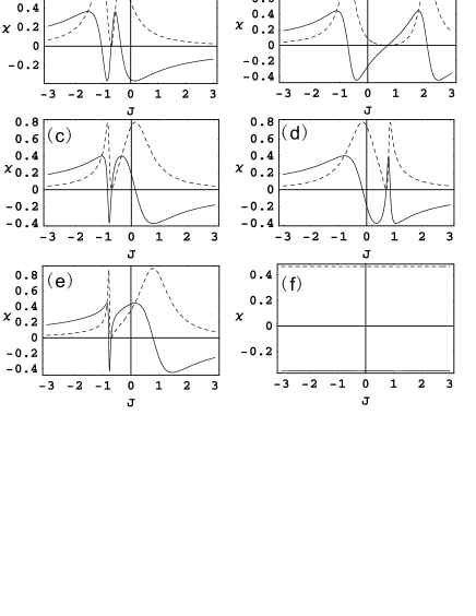
Figure 6: Real (solid) and imaginary (dotted) parts of the linear susceptibility as a function of the inter-cavity coupling strength $J$. The parameters are set as $G_{1}=1$, $\ell=1$. (a) $g_{2}=0.5$, $\delta_{2}=0$, $\delta=1$ and $k=\pi/4$; (b) $g_{2}=2$, $\delta_{2}=0$, $\delta=-1$ and $k=\pi/4$; (c)$g_{2}=0.5$, $\delta_{2}=1$, $\delta=1$ and $k=\pi/4$; (d)$g_{2}=0.5$, $\delta_{2}=-1$, $\delta=-1$ and $k=\pi/4$; (e)$g_{2}=0.5$, $\delta_{2}=2$, $\delta=1$ and $k=\pi/4$; (f)$g_{2}=0.5$, $\delta_{2}=0$, $\delta=1$ and $k=\pi/2$. $J$ is in units of $\gamma_{A}=1$.

It can be observed that: when the incident pulse is center at $k=\pi/(2\ell)$, the susceptibility is independent of $J$ (see Fig. 6(f)); for the input pulse centered at $k=\pi/(4\ell)$, in the vicinity of a frequency corresponding to the two-photon Raman resonances, the medium made of atoms becomes transparency with respect to the input pulse within the photonic band. By comparing Fig. 6(a) and (b), It can be found that the detuning difference $\delta$ determines the position where the transparency window occurs, and the intensity of the control beam decides the width of the transparency window; it can also be observed from Fig. 5 and Fig. 6 that the larger the detuning $|\delta_{2}|$ is, the broader transparency window the spectra of this system has.

VII Conclusion and remarks

We have studied a hybrid system, which consists of $N$ homogeneously coupled resonators with three-level $\Lambda$-type atoms doped in each cavity. The electromagnetically induced transparency (EIT) effect can enhance the ability for coherent manipulations on the photon propagation in the CROW, namely, the photon transmission along the CROW can be well controlled by the amplitude of the driving field. With these results, it is expected that the quantum information encoded in the input pulse can be stored and retrieved by adiabatically tuning $g_{2}$ from $g_{2}\ll G_{1}$ to $g_{2}\gg G_{1}$.

Also it can be seen that our hybrid architecture possesses more controllable parameters for transferring photons in an array of coupled cavities: two coupling strength $g_{1}$, $g_{2}$ and two detunings. Typically, in two photon resonance, the light can be stopped only by controlling the amplitude of the classical field. In comparison with our scheme, the all optical architecture with the passive optical resonator Fanprl04 only has two controllable parameters, the coupling strength between the side-coupled cavity and each of the CROW and the detuning between resonance frequency of side-coupled cavity and that of cavity which constitute the CROW. In other hand, the standard EIT approach only uses the single ”cavity ” and thus there is not a controllable photonic band structure. The on-chip periodic structure used here actually can implement the EIT manipulation for photonic storage in the periodic lattice fixing atoms spatially sunprl91 .

This work is supported by the NSFC with grant Nos. 90203018, 10474104 and 60433050, and NFRPC with Nos. 2006CB921206 and 2005CB724508. The author Lan Zhou gratefully acknowledges the support of K. C. Wong Education Foundation, Hong Kong.

References

- (1) S. E. Harris, Phys. Today 50, No. 7, 36 (1997);
- (2) M. Fleischhauer and M. D. Lukin, Phys. Rev. Lett. 84, 5094 (2000).
- (3) L. V. Hau, S. E. Harris, Z. Dutton, and C. H. Beroozi, Nature 397, 594 (1999);
- (4) S. E. Harris and L. V. Hau, Phys. Rev. Lett. 82, 4611 (1999).
- (5) Q. Xu, S. Sandhu, M. L. Povinelli, J. Shakya, S. Fan, and M. Lipson, Phys. Rev. Lett. 96, 123901 (2006).
- (6) R. W. Boyd, D. J. Gauthier, Nature 441, 701 (2006).
- (7) M. F. Yanik and S. Fan, Phys. Rev. Lett. 92, 083901 (2004).
- (8) M. F. Yanik and S. Fan, Phys. Rev. A 71 013803(2005).
- (9) L. Maleki, A. B. Matsko, A. A. Savchenkov, V. S. Ilchenko, Opt. Lett. 29, 626 (2004).
- (10) Z. S. Yang, N. H. Kwong, R. Binder and A. L. Smirl, J. Opt. Soc. Am. B 22, 2144 (2005).
- (11) D. G. Angelakis, M. F. Santos, and S. Bose, e-print arXiv:quant-ph/0606159.
- (12) M. J. Hartmann, F. G. S. L. Brandao and M. B. Plenio, Nature Physics 2, 849 (2006).
- (13) D. Greentree, C. Tahan, J. H. Cole, L. C. L. Hollenberg, Nature Physics 2, 856 (2006).
- (14) L. Zhou, Y. B. Gao, Z. Song and C. P. Sun, e-print arXiv:cond-mat/0608577, (2006).
- (15) A. Wallraff, D. I. Schuster, A. Blais, L. Frunzio, R.- S. Huang, J. Majer, S. Kumar, S. M. Girvin and R. J. Schoelkopf, Nature 431, 162 (2004);
- (16) A. Blais, R.-S. Huang, A. Wallraff, S. M. Girvin, and R. J. Schoelkopf, Phys. Rev. A 69, 062320 (2004).
- (17) F. M. Hu, L. Zhou, T. Shi and C. P. Sun, e-print arXiv:quant-ph/0610250, submitted to Phys. Rev. E.
- (18) G. R. Jin, P. Zhang, Y. Liu, and C. P. Sun, Phys. Rev. B 68, 134301 (2003).
- (19) J. B. Khurgin, J. Opt. Soc. Am. B 22, 1062 (2005).
- (20) N. Stefanou and A. Modinos, Phys. Rev. B 57, 12127 (1998).
- (21) M. Bayindir, B. Temelkuran, and E. Ozbay, Phys. Rev. Lett. 84, 2140 (2000).
- (22) S. M. Spillane, T. J. Kippenberg, K. J. Vahala, K. W. Goh, E. Wilcut, and H. J. Kimble, Phys. Rev. A 71, 013817 (2005).
- (23) Z. Song, P. Zhang, T. Shi, and C.P. Sun, Phys. Rev. B 71, 205314 (2005).
- (24) S. H. Autler and C. H. Townes, Phys. Rev. 100, 703 (1955).
- (25) U. Fano, Phys. Rev. 124, 1866 (1961).
- (26) C. P. Sun, Y. Li and X. F. Liu, Phys. Rev. Lett. 91, 147903 (2003).
- (27) Y. Li, C. P. Sun, Phys. Rev. A 69, 051802(R) (2004).
- (28) M. O. Scully and M. S. Zubairy, Quantum Optics (Cambridge University Press, Cambridge, 1997).