On the role of entanglement and correlations in mixed-state quantum computation

Abstract

In a quantum computation with pure states, the generation of large amounts of entanglement is known to be necessary for a speed-up with respect to classical computations. However, examples of quantum computations with mixed states are known, such as the DQC1 model [E. Knill and R. Laflamme, Phys. Rev. Lett. 81, 5672 (1998)], in which entanglement is at most marginally present, and yet a computational speed-up is believed to occur. Correlations, and not entanglement, have been identified as a necessary ingredient for mixed-state quantum computation speed-ups. Here we show that correlations, as measured through the operator Schmidt rank, are indeed present in large amounts in the DQC1 circuit. This provides evidence for the preclusion of efficient classical simulation of DQC1 by means of a whole class of classical simulation algorithms, thereby reinforcing the conjecture that DQC1 leads to a genuine quantum computational speed-up.

I Introduction

Quantum computation owes its popularity to the realization, more than a decade ago, that the factorization of large numbers can be solved exponentially faster by evolving quantum systems than via any known classical algorithm Shor . Since then, progress in our understanding of what makes quantum evolutions computationally more powerful than a classical computer has been scarce. A step forward, however, was achieved by identifying entanglement as a necessary resource for quantum computational speed-ups. Indeed, a speed-up is only possible if in a quantum computation, entanglement spreads over an adequately large number of qubits Jozsa99 . In addition, the amount of entanglement, as measured by the Schmidt rank of a certain set of bipartitions of the system, needs to grow sufficiently with the size of the computation v03 . Whenever either of these two conditions is not met, the quantum evolution can be efficiently simulated on a classical computer. These conditions (which are particular examples of subsequent, stronger classical simulation results based on tree tensor networks (TTN) TTN ) are only necessary, and thus not sufficient, so that the presence of large amounts of entanglement spreading over many qubits does not guarantee a computational speed-up, as exemplified by the Gottesman-Knill theorem nc00 .

The above results refer exclusively to quantum computations with pure states. The scenario for mixed-state quantum computation is rather different. The intriguing deterministic quantum computation with one quantum bit (DQC1 or ‘the power of one qubit’) kl98 involves a highly mixed state that does not contain much entanglement dfc05 and yet it performs a task, the computation with fixed accuracy of the normalized trace of a unitary matrix, exponentially faster than any known classical algorithm. This also provides an exponential speedup over the best known classical algorithm for simulations of some quantum processes pklo04 . Thus, in the case of a mixed-state quantum computation, a large amount of entanglement does not seem to be necessary to obtain a speed-up with respect to classical computers.

A simple, unified explanation for the pure-state and mixed-state scenarios is possible v03 by noticing that the decisive ingredient in both cases is the presence of correlations. Indeed, let us consider the Schmidt decomposition of a vector $|\Psi\rangle$, given by

$$|\Psi\rangle=\sum_{i=1}^{\chi}\lambda_{i}|i_{A}\rangle\otimes|i_{B}\rangle,$$ (1)

where $\mbox{$\langle i_{A}|j_{A}\rangle$}=\mbox{$\langle i_{B}|j_{B}\rangle$}=\delta_{ij}$ and $\chi$ is the rank of the reduced density matrices $\rho_{A}\equiv{\rm{Tr}}_{B}[\mbox{$|\psi\rangle\!\langle\psi|$}]$ and $\rho_{B}\equiv{\rm{Tr}}_{A}[\mbox{$|\psi\rangle\!\langle\psi|$}$]; and the (operator) Schmidt decomposition of a density matrix $\rho$ given by zv04

$$\rho=\sum_{i=1}^{\chi^{\sharp}}\lambda^{\sharp}_{i}~{}O_{iA}\otimes O_{iB},$$ (2)

where ${\rm{Tr}}(O_{iA}^{\dagger}O_{jA})={\rm{Tr}}(O_{iB}^{\dagger}O_{jB})=\delta_{ij}$. The Schmidt ranks $\chi$ and $\chi^{\sharp}$ are a measure of correlations between parts $A$ and $B$, with $\chi^{\sharp}=\chi^{2}$ if $\rho=\mbox{$|\Psi\rangle\!\langle\Psi|$}$. Let the density matrix $\rho_{t}$ denote the evolving state of the quantum computer during a computation. Notice that $\rho_{t}$ can represent both pure and mixed states. Then, as shown in Refs. v03 and TTN , the quantum computation can be efficiently simulated on a classical computer using a TTN decomposition if the Schmidt rank $\chi^{\sharp}$ of $\rho$ according to a certain set of bipartitions $A:B$ of the qubits scales polynomially with the size of the computation. In other words, a necessary condition for a computational speed-up is that correlations, as measured by the Schmidt rank $\chi^{\sharp}$, grow super-polynomially in the number of qubits. In the case of pure states (where $\chi=\sqrt{\chi^{\sharp}}$) these correlations are entirely due to entanglement, while for mixed states they may be quantum or classical.

Our endeavor in this paper is to study the DQC1 model of quantum computation following the above line of thought. In particular, we elucidate whether DQC1 can be efficiently simulated with any classical algorithm, such as those in v03 ; TTN (and, implicitly, in Jozsa99 ), that exploits limits on the amount of correlations, in the sense of a small $\chi^{\sharp}$ according to certain bipartitions of the qubits. We will argue here that the state $\rho_{t}$ of a quantum computer implementing the DQC1 model displays an exponentially large $\chi^{\sharp}$, in spite of it containing only a small amount of entanglement dfc05 . We will conclude, therefore, that none of the simulation techniques mentioned above can be used to efficiently simulate ‘the power of one qubit’.

On the one hand, our result indicates that a large amount of classical correlations are behind the (suspected) computational speed-up of DQC1. On the other hand, by showing the failure of a whole class of classical algorithms to efficiently simulate this mixed-state quantum computation, we reinforce the conjecture that DQC1 leads indeed to an exponential speed-up. We note, however, that our result does not rule out the possibility that this circuit could be simulated efficiently using some other classical algorithm.

II DQC1 and Tree Tensor Networks (TTN)

The DQC1 model, represented in Eq. (3), provides an estimate of the normalized trace ${\rm{Tr}}(U_{n})/2^{n}$ of a $n$-qubit unitary matrix $U_{n}\in\mathbb{U}(2^{n})$ with fixed accuracy efficiently kl98 . For discussions on the classical complexity of evaluating the normalized trace of a unitary matrix, see dfc05 .

(3)

This quantum circuit transforms the highly-mixed initial state $\rho_{0}\equiv\mbox{$|0\rangle\!\langle 0|$}\otimes I_{n}/2^{n}$ at time $t=0$ into the final state $\rho_{T}$ at time $t=T$,

$$\rho_{T}=\frac{1}{2^{n+1}}\left(\begin{array}[]{cc}I_{n}&U^{\dagger}_{n}\\ U_{n}&I_{n}\\ \end{array}\right),$$ (4)

through a series of intermediate states $\rho_{t}$, $t\in[0,T]$. The simulation algorithms relevant in the present discussion Jozsa99 ; v03 ; TTN require that $\rho_{t}$ be efficiently represented with a TTN TTN (or a more restrictive structure, such as a product of $k$-qubit states for fixed $k$ Jozsa99 or a matrix product state v03 ) at all times $t\in[0,T]$. Here we will show that the final state $\rho_{T}$, henceforth denoted simply by $\rho$, cannot be efficiently represented with a TTN. This already implies that none of the algorithms in Jozsa99 ; v03 ; TTN can be used to efficiently simulate the DQC1 model.

Storing and manipulating a TTN requires computational space and time that grows linearly in the number of qubits $n$ and as a small power of its rank $q$. The rank $q$ of a TTN is the maximum Schmidt rank $\chi^{\sharp}_{i}$ over all bipartitions $A_{i}:B_{i}$ of the qubits according to a given tree graph whose leaves are the qubits of our system. See TTN for details. The key observation of this paper is that for a typical unitary matrix $U_{n}$, the density matrix $\rho$ in Eq. (4) is such that any TTN decomposition has exponentially large rank $q$. By typical, here we mean a unitary matrix $U_{n}$ efficiently generated through a (random) quantum circuit. That is, $U_{n}$ is the product of poly($n$) one-qubit and two-qubit gates. In the next section we present numerical results that unambiguously suggest that, indeed, typical $U_{n}$ necessarily lead to TTN with exponentially large rank $q$.

We notice that the results of the next section do not exclude the possibility that the quantum computation in the DQC1 model can be efficiently simulated with a TTN for particular choices of $U_{n}$. For instance, if $U_{n}$ factorizes into single-qubit gates, then $\rho$ can be seen to be efficiently represented with a TTN of rank 3, and we can not rule out an efficient simulation of the power of one qubit for that case. Of course, this is to be expected, given that the trace of such $U_{n}$ can be computed efficiently in the first place.

III Exponential growth of Schmidt ranks

In this section we study the rank $q$ of any TTN for the final state $\rho$ of the DQC1 circuit, Eq. (4). We numerically determine that a lower bound to such a rank grows exponentially with the number of qubits $n$.

The Schmidt rank $\chi$ of a pure state $|\rho_{\phi_{A}\psi_{B}}\rangle$

$$|\rho_{\phi_{A}\psi_{B}}\rangle\equiv\rho|\phi_{A}\rangle|\psi_{B}\rangle=\sum_{i=1}^{\chi^{\sharp}}\lambda^{\sharp}_{i}~{}O_{iA}|\phi_{A}\rangle\otimes O_{iB}|\psi_{B}\rangle$$ (5)

obtained by applying the density matrix $\rho$ onto a product state $|\phi_{A}\rangle|\psi_{B}\rangle$ is a lower bound on the operator Schmidt rank $\chi^{\sharp}$ of $\rho$, i.e., $\chi^{\sharp}\geq\chi$. For the purpose of our numerics, we consider the pure state $U_{n}|0\rangle^{\otimes n}$. We build $U_{n}$ as a sequence of $2n$ random two-qubit gates, applied to pairs of qubits, also chosen at random. The random two-qubit unitaries are generated using the mixing algorithm presented in ewslc03 . Note that applying $2n$ gates means that the resulting unitary is efficiently implementable, a situation for which the DQC1 model is valid. For an even number of qubits $n$, we calculate the smallest Schmidt rank $\chi$ over all $n/2:n/2$ partitions of the qubits (similar results can be obtained for odd $n$). The resulting numbers are plotted in Fig (1).

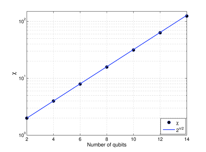
Figure 1: (Color Online):Lower bound for the operator Schmidt rank $\chi^{\sharp}$ of the DQC1 state for any equipartition $n/2:n/2$, as given by the Schmidt rank $\chi$ of the pure state in Eq. (5). The dots are for even numbers of qubits, and the fit is the line $2^{n/2}$. $\chi$ is calculated for a pure state obtained by applying $2n$ random 2-qubit gates on the state $|0\rangle^{\otimes n}$. This is evidence that for a typical unitary $U_{n}$, the rank $q$ of any TTN for the DQC1 state $\rho$ in Eq. (4) grows exponentially with $n$.

The above numerical results strongly suggest that the final state $\rho$ in the DQC1 circuit has exponential Schmidt rank for a typical unitary $U_{n}$. We are not able to provide a formal proof of this fact. This is due to a general difficulty in describing properties of the set $\mathbb{U}_{qc}(2^{n})$ of unitary matrices that can be efficiently realized through a quantum computation. Instead, the discussion is much simpler for the set $\mathbb{U}(2^{n})$ of generic $n$-qubit unitary matrices, where it is possible to prove that $\rho$ cannot be efficiently represented with a TTN for a Haar generated $U_{n}\in\mathbb{U}(2^{n})$, as discussed in the next section. Notice that Ref. ell05 claims that random (but efficient) quantum circuits generate random $n$-qubit gates $U_{n}\in\mathbb{U}_{qc}(2^{n})$ according to a measure that converges to the Haar measure in $\mathbb{U}(2^{n})$. Combined with the theorem in the next section, this would constitute a formal proof of the otherwise numerically evident exponential growth of the rank $q$ of any TTN for the DQC1 final state $\rho$.

IV A formal proof for the Haar-distributed case

Our objective in this section is to analyze the Schmidt rank $\chi^{\sharp}$ of the density matrix $\rho$ in Eq. (4) for certain bipartitions of the $n+1$ qubits, assuming that $U_{n}\in\mathbb{U}(2^{n})$ is Haar-distributed.

It is not difficult to deduce that for any tree of the $n+1$ qubits, there exists at least one edge that splits the tree in two parts $A$ and $B$, with $n_{A}$ and $n_{B}$ qubits, where $n_{0}=\min(n_{A},n_{B})$ fulfills $n/5\leq n_{0}\leq 2n/5$. In other words, if a rank-$q$ TTN exists for the $\rho$ in Eq. (4), then there is a bipartition of the $n+1$ qubits with $n_{0}$ qubits on either $A$ or $B$ and such that the Schmidt rank $\chi^{\sharp}\leq q$. Theorem 1, our main technical result, shows that if $U_{n}$ is chosen randomly according to the Haar measure, then the Schmidt rank of any such bipartition fulfills $\chi^{\sharp}\geq O(2^{n_{0}})$. Therefore for a randomly generated $U_{n}\in\mathbb{U}(2^{n})$, a TTN for $\rho$ has rank $q$ (and computational cost) exponential in $n$, and none of the techniques of Jozsa99 ; v03 ; TTN can simulate the outcome of the DQC1 model efficiently.

Consider now any bipartition $A:B$ of the $n+1$ qubits, where $A$ and $B$ contain $n_{A}$ and $n_{B}$ qubits, with the minimum $n_{0}$ of those restricted by $n/5\leq n_{0}\leq 2n/5$. Without loss of generality we can assume that the top qubit lies in $A$. Actually, we can also assume that $A$ contains the top $n_{A}$ qubits. Indeed, suppose $A$ does not have the $n_{A}$ top qubits. Then we can use a permutation $P_{n}$ on all the $n$ qubits to bring the $n_{A}$ qubits of $A$ to the top $n_{A}$ positions. This will certainly modify $\rho$, but since

$$\left(\begin{array}[]{cc}P_{n}&0\\ 0&P_{n}\\ \end{array}\right)\left(\begin{array}[]{cc}I_{n}&U^{\dagger}_{n}\\ U_{n}&I_{n}\\ \end{array}\right)\left(\begin{array}[]{cc}P^{T}_{n}&0\\ 0&P^{T}_{n}\\ \end{array}\right)=\left(\begin{array}[]{cc}I_{n}&V^{\dagger}_{n}\\ V_{n}&I_{n}\\ \end{array}\right)$$ (6)

where $V_{n}=P_{n}U_{n}P^{T}_{n}$ is another Haar-distributed unitary, we obtain that the new density matrix is of the same form as $\rho$. Finally, in order to ease the notation, we will assume that $n_{A}=n_{0}$ (identical results can be derived for $n_{B}=n_{0}$). Thus $n/5\leq n_{A}\leq 2n/5$.

We note that

$$\left(\begin{array}[]{cc}I_{n}&U^{\dagger}_{n}\\ U_{n}&I_{n}\\ \end{array}\right)=\mathbb{I}_{2}\otimes\mathbb{I}_{n}+\left(\begin{array}[]{cc}0&1\\ 0&0\\ \end{array}\right)\otimes U_{n}^{\dagger}+\left(\begin{array}[]{cc}0&0\\ 1&0\\ \end{array}\right)\otimes U_{n},$$ (7)

so that if we multiply $\rho$ by the product state

$$|\phi_{\vec{\alpha}}\rangle\equiv|t,i,j\rangle\equiv|t,i_{A}\rangle|j_{B}\rangle,$$ (8)

where $\vec{\alpha}\equiv(t,i,j)$, $t=0,1$; $i=1,\dots d_{A}$; $j=1,\dots d_{B}$, we obtain $|\psi_{\vec{\alpha}}\rangle\equiv\rho|\phi_{\vec{\alpha}}\rangle$ where

$$|\psi_{\vec{\alpha}}\rangle=\left\{\begin{array}[]{c}\frac{1}{2^{n+1}}(|0,i,j\rangle+|1\rangle\otimes U_{n}|i,j\rangle)~{}~{}~{}\mbox{if}~{}t=0\\ \frac{1}{2^{n+1}}(|1,i,j\rangle+|0\rangle\otimes U_{n}^{\dagger}|i,j\rangle)~{}~{}~{}\mbox{if}~{}t=1\end{array}\right.$$ (11)

This also justifies our choice of the pure state used in the numerical calculations in the previous section.

Let us consider now the reduced density matrix

$$\sigma^{B}_{\vec{\alpha}} \equiv {\rm{Tr}}_{A}[\mbox{$|\psi_{\vec{\alpha}}\rangle\!\langle\psi_{\vec{\alpha}}|$}]$$ (12)

$$= \frac{1}{2^{n+1}}\left(|j\rangle{\langle j|}+{\rm{Tr}}_{A}[U_{n}|i,j\rangle{\langle i,j|}U_{n}^{\dagger}]\right)$$

for $t=0$ (for $t=1$, $U_{n}$ and $U_{n}^{\dagger}$ need to be exchanged). For a unitary matrix $U_{n}$ randomly chosen according to the Haar measure on $\mathrm{U}(n)$, $U_{n}|i,j\rangle$ is a random pure state on $A\otimes B$. Here, and henceforth $A$ is the space of the first $n_{A}$ qubits without the top qubit. It follows from hlw06 that the operator

$$Q={\rm{Tr}}_{A}[U_{n}|i,j\rangle{\langle i,j|}U_{n}^{\dagger}]$$ (13)

has rank $d_{A}$. Therefore the rank of $\sigma^{B}_{\vec{\alpha}}$ (equivalently, the Schmidt rank $\chi$ of $|\psi_{\vec{\alpha}}\rangle$) is at least $2^{n_{0}}$. From Eq. (5) we conclude that the Schmidt rank of $\rho$ fulfills $\chi^{\sharp}\geq 2^{n_{0}}\geq 2^{n/5}$. We can now collate these results into

Theorem 1

Let $U_{n}$ be an $n$-qubit unitary transformation chosen randomly according to the Haar measure on $\mathrm{U}(2^{n})$, and let $A:B$ denote a bipartition of $n+1$ qubits into $n_{A}$ and $n_{B}$ qubits, where $n_{0}\equiv\min(n_{A},n_{B})$. Then $n/5\leq n_{0}\leq 2n/5$ and the Schmidt decomposition of $\rho$ in Eq. (4) according to bipartition $A:B$ fulfills $\chi^{\sharp}\geq 2^{n/5}$.

We have seen that we cannot efficiently simulate DQC1 with an algorithm that relies on having a TTN for $\rho$ with low rank $q$. However, in order to make this result robust, we need to also show that $\rho$ canot be well approximated by another $\tilde{\rho}$ accepting an efficient TTN. We do this in Appendix A.

V Conclusions

The results in this paper show that the algorithms of Jozsa99 ; v03 ; TTN are unable to efficiently simulate a DQC1 circuit. The efficiency of a quantum simulation using these algorithms relies on the possibility of efficiently decomposing the state $\rho$ of the quantum computer using a TTN. We have seen that for the final state of the DQC1 circuit no efficient TTN exists.

It is also interesting to note that the numerics and Theorems 1 and 2 in this paper can be generalized for any fixed polarization $\tau$, ($0<\tau\leq 1$) of the initial state $\tau\mbox{$|0\rangle\!\langle 0|$}+(1-\tau)\mathbb{I}/2$ of the top qubit of the circuit in Eq (3), implying that the algorithms of Jozsa99 ; v03 ; TTN are also unable to efficiently simulate the power of even the tiniest fraction of a qubit.

Appendix A Distribution of the Schmidt coefficients

In this Appendix we explore the robustness of the statement of Theorem 1. To this end, we consider the Schmidt rank $\tilde{\chi}^{\sharp}$ for a density matrix $\tilde{\rho}$ that approximates $\rho$ according to a fidelity $F(O_{1},O_{2})$ defined in terms of the natural inner product on the space of linear operators,

$$F(O_{1},O_{2})\equiv{\rm{Tr}}({O_{1}^{\dagger}O_{2}})\Bigg{/}{\sqrt{{\rm{Tr}}(O_{1}^{\dagger}O_{1})}\sqrt{{\rm{Tr}}(O_{2}^{\dagger}O_{2})}},$$

where $F=1$ if and only if $O_{1}=O_{2}$ and $F=|\mbox{$\langle\psi_{1}|\psi_{2}\rangle$}|^{2}$ for projectors $O_{i}=P_{\psi_{i}}$ on pure states $|\psi_{i}\rangle$. We will show that if $\tilde{\rho}$ is close to $\rho$, then $\tilde{\chi}^{\sharp}$ for a bipartition as in Theorem 1 is also exponential. To prove this, we will require a few lemmas which we now present.

Lemma 1

Let $|\Psi\rangle$ be a bipartite vector with $\chi$ terms in its Schmidt decomposition,

$$|\Psi\rangle=N_{\Psi}\!\sum_{i=1}^{\chi}\lambda_{i}|i_{A}\rangle|i_{B}\rangle,~{}~{}\lambda_{i}\geq\lambda_{i+\!1}\geq 0,~{}\sum_{i=1}^{\chi}\lambda_{i}^{2}=1,$$

where $N_{\Psi}\equiv\sqrt{\mbox{$\langle\Psi|\Psi\rangle$}}$, and let $|\Phi\rangle$ be a bipartite vector with norm $N_{\Phi}$ and Schmidt rank $\chi^{\prime}$, where $\chi^{\prime}\leq\chi$. Then,

$$\max_{|\Phi\rangle}|\mbox{$\langle\Psi|\Phi\rangle$}|=N_{\Psi}N_{\Phi}\sqrt{\sum_{i=1}^{\chi^{\prime}}\lambda_{i}^{2}}.$$ (14)

Proof: Let $\mu_{i}$ denote the Schmidt coefficients of $|\Phi\rangle$. It follows from Lemma 1 in vjn00 that $\max_{|\Phi\rangle}|\mbox{$\langle\Psi|\Phi\rangle$}|=N_{\Psi}N_{\Phi}\sum_{i=1}^{\chi^{\prime}}\lambda_{i}\mu_{i},$ and the maximization over $\mu_{i}$ is done next. A straightforward application of the method of Lagrange multipliers provides us with $\mu_{i}=c\lambda_{i},~{}i=1,2,\dots,\chi^{\prime}$ for some constant $c$. Since $\sum_{i=1}^{\chi^{\prime}}\mu_{i}^{2}=1=c^{2}\sum_{i=1}^{\chi^{\prime}}\lambda_{i}^{2}$, $c=1/\sqrt{\sum_{i=1}^{\chi^{\prime}}\lambda_{i}^{2}}.$ Thus,

$$\max_{|\Phi\rangle}|\mbox{$\langle\Psi|\Phi\rangle$}|=cN_{\Psi}N_{\Phi}\sum_{i=1}^{\chi^{\prime}}\lambda_{i}^{2}$$

and the result follows. $\square$

We will also use two basic results related to majorization theory. Recall that, by definition, a decreasingly ordered probability distribution $\vec{p}=(p_{1},p_{2},\dots,p_{d})$, where $p_{\alpha}\geq p_{\alpha+1}\geq 0$, $\sum_{\alpha}p_{\alpha}=1$, is majorized by another such probability distribution $\vec{q}$, denoted $\vec{p}\prec\vec{q}$, if $\vec{q}$ is more ordered or concentrated than $\vec{p}$ (equivalently, $\vec{p}$ is flatter or more mixed than $\vec{q}$) in the sense that the following inequalities are fulfilled:

$$\sum_{\alpha=1}^{k}p_{\alpha}\leq\sum_{\alpha=1}^{k}q_{\alpha}~{}~{}~{}\forall~{}k=1,\dots,d$$ (15)

with equality for $k=d$. The following result can be found in Exercise II.1.15 of Bhatia :

Lemma 2

Let $\rho_{\vec{x}}$ and $\rho_{\vec{y}}$ be density matrices with eigenvalues given by probability distributions $\vec{x}$ and $\vec{y}$. Let $\sigma(M)$ denote the decreasingly ordered eigenvalues of hermitian operator $M$. Then

$$\sigma(\rho_{\vec{x}}+\rho_{\vec{y}})\prec\vec{x}+\vec{y}.$$

The next result follows by direct inspection.

Lemma 3

Let coefficients $\delta_{i}$, $1\leq i\leq d$, be such that $-\delta\leq\delta_{i}\leq\delta$ for some positive $\delta\leq 1$ and $\sum_{i}\delta_{i}=1$, and consider the probability distribution $\vec{p}(\{\delta_{i}\})$,

$$\vec{p}(\{\delta_{i}\})\equiv\left(\frac{1}{2}+\frac{1+\delta_{1}}{2d},\frac{1+\delta_{2}}{2d},\cdots,\frac{1+\delta_{d}}{2d}\right).$$

Then

$$\vec{p}(\{\delta_{i}\})\prec\vec{p}(\{\delta_{i}^{*}\}),$$

where

$$\delta_{i}^{*}\equiv\left\{\begin{array}[]{c}~{}~{}\delta~{}~{}~{}i\leq d/2\\ -\delta~{}~{}~{}i>d/2\end{array}\right.$$

and we assume $d$ to be even.

Finally, we need a result from hlw06 :

Lemma 4

With probability very close to 1,

$$\mathrm{Pr}\Big{[}(1-\delta)\frac{\Upsilon}{d_{A}}\leq Q\leq(1+\delta)\frac{\Upsilon}{d_{A}}\Big{]}$$

$$\geq 1-\left(\frac{10~{}d_{A}}{\delta}\right)^{2d_{A}}2^{(-d_{B}\;\delta^{2}/14\ln 2)}$$

$$\geq 1-O\left(\frac{1}{\exp(\delta^{2}\exp(n))}\right),$$ (16)

where $d_{A}=2^{n_{A}}=2^{n_{0}}$ and $d_{B}=2^{n_{B}}=2^{n-n_{0}+1}$, and the operator $Q$ defined in Eq. (13) is within a ball of radius $\delta$ of a (unnormalized) projector $\Upsilon/d_{A}$ of rank $d_{A}$ [provided $d_{B}$ is a large multiple of $d_{A}\log d_{A}/\delta^{2}$ hlw06 , which is satisfied for large $n$, given that $n/5\leq n_{0}\leq 2n/5$].

Our second theorem uses the fact that the Schmidt decomposition of $\rho$ does not only have exponentially many coefficients, but that these are roughly of the same size.

Theorem 2

Let $\rho$, $U_{n}$, and $A\!:\!B$ be defined as in Theorem 1. If $F(\rho,\tilde{\rho})\geq 1-\epsilon$, then with probability $p(\delta,n)=1-O(\exp(-\delta^{2}\exp(n)))$, the Schmidt rank for $\tilde{\rho}$ according to bipartition $A\!:\!B$ satisfies $\tilde{\chi}^{\sharp}\geq(1-4\epsilon-\delta)2^{n/5}$.

Proof: For any product vector of Eq. (8) we have

$$|{\langle tij|}\rho\tilde{\rho}|tij\rangle| \leq ~{}N_{\vec{\alpha}}~{}\tilde{N}_{\vec{\alpha}}~{}\sqrt{\sum_{k=1}^{\tilde{\chi}^{\sharp}}(\lambda_{k}^{ij})^{2}}$$

$$\leq N_{\vec{\alpha}}~{}\tilde{N}_{\vec{\alpha}}\;g(\tilde{\chi}^{\sharp}/d_{A}),$$

where

$$g(x)\equiv\sqrt{\frac{1+(1+\delta)x}{2}}$$ (18)

and $N_{\vec{\alpha}}\equiv\sqrt{{\langle tij|}\rho^{2}|tij\rangle}$, $\tilde{N}_{\vec{\alpha}}\equiv\sqrt{{\langle tij|}\tilde{\rho}^{2}|tij\rangle}$. The first inequality in (A) follows from Lemma 1, whereas the second one follows from the fact that the spectrum $\vec{p}$ of

$$\rho_{B}\equiv(N_{\vec{\alpha}})^{-2}{\rm{Tr}}_{A}[\rho\mbox{$|tij\rangle\!\langle tij|$}\rho]=\frac{1}{2}(\mbox{$|j\rangle\!\langle j|$}+Q),$$

where $Q$ has all its $d_{A}$ non-zero eigenvalues $q_{i}$ in the interval $2^{-n_{0}}(1-\delta)\leq q_{i}\leq 2^{-n_{0}}(1+\delta)$, is majorized by $\vec{p}(\{\delta_{i}^{*}\})$, as follows from Lemmas 2 and 3. Then,

$$1-\epsilon\leq\frac{{\rm{Tr}}\rho\tilde{\rho}}{\sqrt{{\rm{Tr}}\rho^{2}}\sqrt{{\rm{Tr}}\tilde{\rho}^{2}}}$$

$$= \frac{\sum_{\vec{\alpha}}{\langle\vec{\alpha}|}\rho\tilde{\rho}|\vec{\alpha}\rangle}{\sqrt{\sum_{\vec{\alpha}^{\prime}}{\langle\vec{\alpha}^{\prime}|}\rho^{2}|\vec{\alpha}^{\prime}\rangle\sum_{\vec{\alpha}^{\prime\prime}}{\langle\vec{\alpha}^{\prime\prime}|}\tilde{\rho}^{2}|\vec{\alpha}^{\prime\prime}\rangle}}$$

$$\leq g(\tilde{\chi}^{\sharp}/d_{A})\frac{\sum_{\vec{\alpha}}N_{\vec{\alpha}}\tilde{N}_{\vec{\alpha}}}{\sqrt{\sum_{\vec{\alpha}^{\prime}}(N_{\vec{\alpha}^{\prime}})^{2}\sum_{\vec{\alpha}^{\prime\prime}}(\tilde{N}_{\vec{\alpha}^{\prime\prime}})^{2}}}$$

$$\leq g(\tilde{\chi}^{\sharp}/d_{A}),$$

where in the last step we have used the Cauchy-Schwarz inequality, $|\mbox{$\langle x|y\rangle$}|\leq\sqrt{\mbox{$\langle x|x\rangle$}}\sqrt{\mbox{$\langle y|y\rangle$}}$. The result of the theorem follows from $g(\tilde{\chi}^{\sharp}/2^{n_{0}})\geq 1-\epsilon$. $\square$

References

- (1) P. Shor, Proceedings of the 35th Annual Symposium on Foundations of Computer Science, Santa Fe, NM, 20 to 22 November 1994, S. Goldwasser, Ed. (IEEE Computer Science, Los Alamitos, CA, 1994) p. 124.
- (2) R. Jozsa and N. Linden, Proc. Roy. Soc. Lond. A 459, 2011 (2003).
- (3) G. Vidal, Phys. Rev. Lett. 91, 147902 (2003).
- (4) Y.-Y. Shi, L.-M. Duan, and G. Vidal, Phys. Rev. A 74, 022320 (2006). M. Van den Nest, W. Dür, G. Vidal, H. J. Briegel, Phys. Rev. A 75, 012337 (2006).
- (5) M. Nielsen and I. Chuang, Quantum Computation and Quantum Information (Cambridge University Press, Cambridge, England, 2000).
- (6) E. Knill and R. Laflamme, Phys. Rev. Lett. 81, 5672 (1998).
- (7) A. Datta, S. T. Flammia, and C. M. Caves, Phys. Rev. A 72, 042316 (2005).
- (8) D. Poulin, R. Blume-Kohout, R. Laflamme, and H. Ollivier, Phys. Rev. Lett. 92, 177906 (2004). J. Emerson, S. Lloyd, D. Poulin, and D. Cory, Phys. Rev. A 69, 050305(R) (2004).
- (9) M. Zwolak and G. Vidal, Phys. Rev. Lett. 93, 207205 (2004).
- (10) J. Emerson, Y. S. Weinstein, M. Saraceno, S. Lloyd, and D. G. Cory, Science 302, 2098 (2003).
- (11) J. Emerson, E. Livine, S. Lloyd, Phys. Rev. A 72, 060302 (2005).
- (12) G. Vidal, D. Jonathan, and M. A. Nielsen, Phys. Rev. A 62, 012304 (2000).
- (13) P. Hayden, D. W. Leung, and A. Winter, Commun. Math. Phys. 265, 95 (2006).
- (14) Rajendra Bhatia, Matrix Analysis (Springer-Verlag, New York, 1997).