Sample dependence of the Casimir force

Abstract

We have analyzed available optical data for Au in the mid-infrared range which is important for a precise prediction of the Casimir force. Significant variation of the data demonstrates genuine sample dependence of the dielectric function. We demonstrate that the Casimir force is largely determined by the material properties in the low frequency domain and argue that therefore the precise values of the Drude parameters are crucial for an accurate evaluation of the force. These parameters can be estimated by two different methods, either by fitting real and imaginary parts of the dielectric function at low frequencies, or via a Kramers-Kronig analysis based on the imaginary part of the dielectric function in the extended frequency range. Both methods lead to very similar results. We show that the variation of the Casimir force calculated with the use of different optical data can be as large as 5% and at any rate cannot be ignored. To have a reliable prediction of the force with a precision of 1%, one has to measure the optical properties of metallic films used for the force measurement.

1 Introduction

The Casimir force [1] between uncharged metallic plates attracts considerable attention as a macroscopic manifestation of the quantum vacuum [2, 3, 5, 4, 6]. With the development of microtechnologies, which routinely control the separation between bodies smaller than 1 $\mu m$, the force became a subject of systematic experimental investigation. Modern precision experiments have been performed using different techniques such as torsion pendulum [7], atomic force microscope (AFM) [8, 9], microelectromechanical systems (MEMS) [10, 11, 12, 13, 14, 15] and different geometrical configurations: sphere-plate [7, 9, 12], plate-plate [16] and crossed cylinders [17]. The relative experimental precision of the most precise of these experiments is estimated to be about 0.5% for the recent MEMS measurement [13] and 1% for the AFM experiments [9, 10].

In order to come to a valuable comparison between the experiments and the theoretical predictions, one has to calculate the force with a precision comparable to the experimental accuracy. This is a real challenge to the theory because the force is material, surface, geometry and temperature dependent. Here we will only focus on the material dependence, which is easy to treat on a level of some percent precision but which will turn out difficult to tackle on a high level of precision since different uncontrolled factors are involved.

In its original form, the Casimir force per unit surface [1]

$$F_{c}\left(a\right)=-\frac{\pi^{2}}{240}\frac{\hbar c}{L^{4}}$$ (1)

was calculated between ideal metals. It depends only on the fundamental constants and the distance between the plates $L$. The force between real materials differs significantly from (1) for mirror separations smaller than 1 $\mu$m.

For mirrors of arbitrary material, which can be described by reflection coefficients, the force per unit area can be written as [18]:

$$F = 2\sum_{\mu}\int\frac{\mathrm{d}^{2}\mathbf{k}}{4\pi^{2}}\int_{0}^{\infty}\frac{\mathrm{d}\zeta}{2\pi}\hbar\kappa\frac{r_{\mu}\left[i\zeta,\mathbf{k}\right]^{2}e^{-2\kappa L}}{1-r_{\mu}\left[i\zeta,\mathbf{k}\right]^{2}e^{-2\kappa L}}$$ (2)

$$\kappa=\sqrt{\mathbf{k}^{2}+\frac{\zeta^{2}}{c^{2}}}$$

where $r_{\mu}=(r_{s},r_{p})$ denotes the reflection amplitude for a given polarization $\mu=s,\;p$

$$r_{s} = -\frac{\sqrt{\mathbf{k}^{2}+\varepsilon\left(i\zeta\right)\frac{\zeta^{2}}{c^{2}}}-c\kappa}{\sqrt{\mathbf{k}^{2}+\varepsilon\left(i\zeta\right)\frac{\zeta^{2}}{c^{2}}}+c\kappa}$$

$$r_{p} = \frac{\sqrt{\mathbf{k}^{2}+\varepsilon\left(i\zeta\right)\frac{\zeta^{2}}{c^{2}}}-c\kappa\varepsilon\left(i\zeta\right)}{\sqrt{\mathbf{k}^{2}+\varepsilon\left(i\zeta\right)\frac{\zeta^{2}}{c^{2}}}+c\kappa\varepsilon\left(i\zeta\right)}$$ (3)

The force between dielectric materials had first been derived by Lifshitz [19, 20]. The material properties enter these formulas via the dielectric function $\varepsilon\left(i\zeta\right)$ at angular imaginary frequencies $\omega=i\zeta$, which is related to the physical quantity $\varepsilon^{\prime\prime}\left(\omega\right)=\mathrm{Im}\left(\varepsilon\left(\omega\right)\right)$ with the help of the dispersion relation

$$\varepsilon\left(i\zeta\right)-1=\frac{2}{\pi}\int\limits_{0}^{\infty}d\omega\frac{\omega\varepsilon^{\prime\prime}\left(\omega\right)}{\omega^{2}+\zeta^{2}}.$$ (4)

For metals $\varepsilon^{\prime\prime}\left(\omega\right)$ is large at low frequencies, thus the main contribution to the integral in Eq. (4) comes from the low frequencies even if $\zeta$ corresponds to the visible frequency range. For this reason the low-frequency behavior of $\varepsilon(\omega)$ is of primary importance.

The Casimir force is often calculated using the optical data taken from [21], which provides real and imaginary parts of the dielectric function within some frequency range, typically between 0.1 and $10^{4}$ eV for the most commonly used metals, Au, Cu and Al, corresponding to a frequency interval $[1.519\cdot 10^{14},1.519\cdot 10^{19}]$ rad/s (1 eV=$1.519\cdot 10^{15}$ rad/s ). When the two plates are separated by a distance $L$, one may introduce a characteristic imaginary frequency $\zeta_{\rm ch}=c/2L$ of electromagnetic field fluctuations in the gap. Fluctuations of frequency $\zeta\sim\zeta_{\rm ch}$ give the dominant contribution to the Casimir force. For example, for a plate separation of $L=100$ nm the characteristic imaginary frequency is $\zeta_{\rm ch}=0.988$ eV. Comparison with the frequency interval where optical data is available shows that the high frequency data exceeds the characteristic frequency by 3 orders of magnitude, which is sufficient for the calculation of the Casimir force. However, in the low frequency domain, optical data exists only down to frequencies which are one order of magnitude below the characteristic frequency, which is not sufficient to evaluate the Casimir force. Therefore for frequencies lower than the lowest tabulated frequency, $\omega_{\rm c}$, the data has to be extrapolated. This is typically done by a Drude dielectric function

$$\varepsilon\left(\omega\right)=1-\frac{\omega_{\rm p}^{2}}{\omega\left(\omega+i\omega_{\tau}\right)},$$ (5)

which is determined by two parameters, the plasma frequency $\omega_{\rm p}$ and the relaxation frequency $\omega_{\tau}$.

Different procedures to get the Drude parameters have been discussed in the literature. They may be estimated, for example, from information in solid state physics or extracted form the optical data at the lowest accessible frequencies. The exact values of the Drude parameters are very important for the precise evaluation of the force. Lambrecht and Reynaud [18] fixed the plasma frequency using the relation

$$\omega_{\rm p}^{2}=\frac{Ne^{2}}{\varepsilon_{0}m_{e}^{\ast}},$$ (6)

where $N$ is the number of conduction electrons per unit volume, $e$ is the charge and $m_{e}^{\ast}$ is the effective mass of electron. The plasma frequency was evaluated using the bulk density of Au, assuming that each atom gives one conduction electron and that the effective mass coincides with the mass of the free electron. The optical data at the lowest frequencies were then used to estimate $\omega_{\tau}$ with the help of Eq. (5). In this way the plasma frequency $\omega_{\rm p}=9.0$ eV and the relaxation frequency $\omega_{\tau}=0.035$ eV have been found. This procedure was largely adopted in the following [9, 17, 10, 16, 11]. However, on the example of Cu, it was stressed in [18] that the optical data may vary from one reference to another and a different choice of parameters for the extrapolation procedure to low frequencies can influence the Casimir force significantly.

Boström and Sernelius [23] and Svetovoy and Lokhanin [22] extracted the low-frequency optical data by fitting them with Eq. (5). For one set of data from Ref. [25] the result [22] was close to that found by the first approach, but using different sources for the optical data collected in Ref. [25] an appreciable difference was found [24, 22]. This difference was attributed to the defects in the metallic films which appear as the result of the deposition process. It was indicated that the density of the deposited films is typically smaller and the resistivity larger than the corresponding values for the bulk material. The dependence of optical properties of Au films on the details of the deposition process, annealing, voids in the films, and grain size was already discussed in the literature [26].

In this paper we analyze the optical data for Au from several available sources, where the mid-infrared frequency range was investigated. The purpose is to establish the variation range of the Drude parameters and calculate the uncertainty of the Casimir force due to the variation of existing optical data. This uncertainty is of great importance in view of the recent precise Casimir force measurement [27, 13] which have been performed with high experimental accuracy. On the other hand, sophisticated theoretical calculations predict the Casimir force at the level of 1% or better. These results illustrate the considerable progress achieved in the field in only one decade. In order to assure a comparison between theory and experiment at the same level of precision, one has to make sure that the theoretical calculation considers precisely the same system investigated in the experiment. This is the key point we want to address in our paper. With our current investigation we find an intrinsic force uncertainty of the order of 5% coming from the fact that the Drude parameters are not precisely known. These parameters may vary from one sample to another, depending on many details of the preparation conditions. In order to assure a comparison at the level of 1% or better between theoretical predictions and experimental results for the Casimir force, the optical properties of the mirrors have to be measured in the experiment.

The paper is organized as follows. In Sec. 2 we explain and discuss the importance of the precise values of the Drude parameters. In Sec. 3 the existing optical data for gold are reviewed and analyzed. The Drude parameters are extracted from the data by fitting both real and imaginary parts of the dielectric function at low frequencies in Sec. 4. In Section 5 the Drude parameters are estimated by a different method using Kramers-Kroning analysis. The uncertainty in the Casimir force due to the sample dependence is evaluated in Sec. 6 and we present our conclusions in Sec. 7.

2 Importance of the values of the Drude parameters

In Figure 1 (left) we present a typical plot of the imaginary part of the dielectric function, which comprises Palik’s Handbook data for gold [21]. The solid line shows the actual data taken from two original sources: the points to the right of the arrow are those by Thèye [28] and to the left by Dold and Mecke [29]. No data is available for frequencies smaller than the cutoff frequency $\omega_{\rm c}$ ($0.125$ eV for this data set) and $\varepsilon^{\prime\prime}\left(\omega\right)$ has to be extrapolated into the region $\omega<\omega_{\rm c}$. The dotted line shows the Drude extrapolation with the parameters $\omega_{\rm p}=9.0$ eV and $\omega_{\tau}=0.035$ eV obtained in Ref. [18].

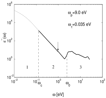
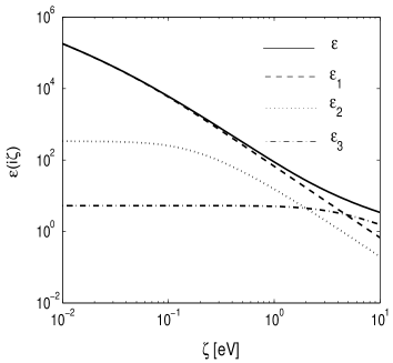
Figure 1: Left panel: Palik’s Handbook data for Au [21] (solid line) extrapolated to low frequencies (dotted line) with the Drude parameters indicated in the corner. Right panel: contributions of different real frequency domains to the dielectric function on the imaginary axis $\varepsilon(i\zeta)$.

One can separate three frequency regions in Fig. 1 (left panel). The region marked as 1 corresponds to the frequencies smaller than $\omega_{\rm c}$. The region 2 defining the Drude parameters extends from the cutoff frequency to the edge of the interband absorption $\omega_{0}$. The high energy domain $\omega>\omega_{0}$ is denoted by 3.

We may now deduce the dielectric function at imaginary frequencies (4) using the Kramers-Kronig relation

$$\varepsilon\left(i\zeta\right)=1+\varepsilon_{1}\left(i\zeta\right)+\varepsilon_{2}\left(i\zeta\right)+\varepsilon_{3}\left(i\zeta\right),$$ (7)

where the indices 1, 2, and 3 indicate respectively the integration ranges $0\leq\omega<\omega_{\rm c}$, $\omega_{\rm c}\leq\omega<\omega_{0}$, and $\omega_{0}\leq\omega<\infty$. $\varepsilon_{1}$ can be derived using the Drude model (5) leading to

$$\varepsilon_{1}\left(i\zeta\right)=\frac{2}{\pi}\frac{\omega_{p}^{2}}{\zeta^{2}-\omega_{\tau}^{2}}\left[\tan^{-1}\left(\frac{\omega_{c}}{\omega_{\tau}}\right)-\frac{\omega_{\tau}}{\zeta}\tan^{-1}\left(\frac{\omega_{c}}{\zeta}\right)\right].$$ (8)

The two other functions $\varepsilon_{2}$ and $\varepsilon_{3}$ have to be calculated numerically. The results for all three functions as well as for $\varepsilon\left(i\zeta\right)$ are shown in Fig. 1 (right). One can clearly see that $\varepsilon_{1}\left(i\zeta\right)$ dominates the dielectric function at imaginary frequencies up to $\zeta\approx 5$ eV. $\varepsilon_{2}\left(i\zeta\right)$ gives a perceptible contribution to $\varepsilon\left(i\zeta\right)$, while $\varepsilon_{3}\left(i\zeta\right)$ produces minor contribution negligible for $\zeta<0.5$ eV.

As mentioned in the Introduction, we may introduce a characteristic imaginary frequency $\zeta_{\rm ch}=c/2L$ of field fluctuations which give the dominant contribution to the Casimir force between two plates at a distance $L$. For a plate separation of $L=100$ nm the characteristic imaginary frequency is $\zeta_{\rm ch}=0.988$ eV. At this frequency the contributions of different frequency domains to $\varepsilon\left(i\zeta_{ch}\right)$ are $\varepsilon_{1}=68.42$, $\varepsilon_{2}=15.65$, and $\varepsilon_{3}=5.45$. This means that for all experimentally investigated situations, $L\gtrsim 100$ nm, region 1, corresponding to the extrapolated optical data, gives the main contribution to $\varepsilon\left(i\zeta\right)$. It is therefore important to know precisely the Drude parameters.

3 Analysis of different optical data for gold

The optical properties of gold were extensively investigated in 50-70th. In many of those works the importance of sample preparation methods was recognized and carefully discussed. A complete bibliography of the publications up to 1981 can be found in Ref. [30]. Regrettably the contemporary studies of gold nanoclusters produce data inappropriate for our purposes. Among recent experiments let us mention the measurement of normal reflectance for evaporated gold films [31], which was performed in the wide wavelength range $0.3-50$ $\mu$m, but unfortunately does not permit to evaluate independently both real and imaginary parts of the dielectric function. In contrast, the use of new ellipsometric techniques [32, 33] has produced data for the real and imaginary part of the dielectric function for energy intervals $1.5-4.5$ eV [34] and $1.5-3.5$ eV [35].

A significant amount of data in the interband absorption region (domain 3) has been obtained by different methods under different conditions [36, 28, 37, 38, 39, 34, 35]. Though this frequency band is not very important for the Casimir force, it provides information on how the data may vary from one sample to another. On the contrary there are only a few sources where optical data was collected in the mid-infrared (domain 2) and from which the dielectric function can be extracted. The data available for $\varepsilon^{\prime}\left(\omega\right)$ and $\varepsilon^{\prime\prime}\left(\omega\right)$ in the range $\omega<1.5$ eV and interband absorption domain 3 are presented respectively in the left and right graph of Fig. 2. These data sets demonstrate considerable variations of the dielectric function from one sample to another.

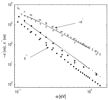
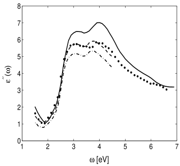
Figure 2: Left panel: Available optical data in the mid-infrared region. The dots represent the Dold and Mecke data for $\omega<1$ eV [29] and Thèye data [28] for higher frequencies. The squares denote the Weaver data [30]. The circles stand for the data from [40]. The triangles represent the data [41]. Solid squares, circles, and triangles are used to mark $\varepsilon^{\prime\prime}\left(\omega\right)$ while the open symbols are used for $\varepsilon^{\prime}\left(\omega\right)$. Right panel: $\varepsilon^{\prime\prime}(\omega)$ in the interband region for different samples. The solid line represents the data measured with the well annealed bulk-like film by Thèye [28]. The dots are the data by Johnson and Christy [37] found for unannealed films. The dashed and dash-dotted lines are recent data sets by Wang et al. [34] for unannealed films. They correspond to films deposited with e-beam and thermal evaporation methods, respectively.

Let us briefly discuss the sets of data [21, 30, 40, 41] used in our analysis and the corresponding samples. The commonly used Handbook of Optical Constants of Solids [21] comprises the optical data covering the region from $0.125$ to $9184$ eV (dots in Fig. 2). The experimental points are assembled from several sources. For $\omega<1$ eV they are reported by Dold and Mecke [29]. For higher frequencies up to $6$ eV they correspond to the Thèye data [28]. Dold and Mecke give only little information about the sample preparation, reporting that the films were evaporated onto a polished glass substrate and measured in air by using an ellipsometric technique [29]. Annealing of the samples was not reported.

Thèye [28] described her films very carefully. The samples were semitransparent Au films with a thickness of $100-250$ Å evaporated in ultrahigh vacuum on supersmooth fused silica. The substrate was kept in most cases at room temperature. After the deposition the films were annealed in the same vacuum at $100-150^{\circ}$ C. The structure of the films was investigated by X-ray and transmission-electron-microscopy methods. The dc resistivity of the films was found to be very sensitive to the preparation conditions. The errors in the optical characteristics of the films were estimated on the level of a few percents.

The handbook [30] embraces the optical data from $0.1$ eV to $28.6$ eV (marked with squares in Fig. 2). The data in the domain $\omega<4$ eV is provided by Weaver et al. [30]. The values of $\varepsilon(\omega)$ were found for the electropolished bulk Au(110) sample. Originally the reflectance was measured in a broad interval $0.1\leq\omega\leq 30$ eV and then the dielectric function was determined by a Kramers-Kronig analysis. Due to indirect determination of $\varepsilon$ the recommended accuracy of these data sets is only 10%.

The optical data of Motulevich and Shubin [40] for Au films is marked with circles in Fig. 2. In this paper the films were carefully described. Gold was evaporated on polished glass at a pressure of $\sim 10^{-6}$ Torr. The investigated films were $0.5-1\ \mu$m thick. The samples were annealed in the same vacuum at $400^{\circ}$ C for more than 3 hours. The optical constants $n$ and $k$ ($n+ik=\sqrt{\varepsilon}$) were measured by polarization methods in the spectral range $1-12\ \mu$m. The errors in $n$ and $k$ were estimated as 2-3% and 0.5-1%, respectively.

Finally, the triangles represent Padalka and Shklarevskii data [41] for unannealed Au films evaporated onto glass.

The variation of the data points from different sources cannot be explained by experimental errors. The observed deviation is the result of different preparation procedures and reflects genuine difference between samples. The deposition method, type of the substrate, its temperature, quality and the deposition rate influence the optical properties. When we are speaking about a precise comparison between theory and experiment for the Casimir force at the level of 1% or better, there is no such material as gold in general any more. There is only a gold sample prepared under definite conditions.

4 Evaluation of the Drude parameters through extrapolation

We will now use the available data in the mid-infrared region to extrapolate into the low frequency range. If the transition between inter- and intraband absorption in gold is sharp, the data below $\omega_{0}$ should be well described by the Drude function

$$\varepsilon^{\prime}\left(\omega\right)=1-\frac{\omega_{p}^{2}}{\omega^{2}+\omega_{\tau}^{2}},\ \ \varepsilon^{\prime\prime}\left(\omega\right)=\frac{\omega_{p}^{2}\omega_{\tau}}{\omega\left(\omega^{2}+\omega_{\tau}^{2}\right).}$$ (9)

For $\omega\gg\omega_{\tau}$, the data on the log-log plot should fit straight lines with the slopes $-2$ and $-3$ for $\varepsilon^{\prime}$ and $\varepsilon^{\prime\prime}$, respectively, shifted along the ordinate due to variation of the parameters for different samples. The data points in the right graph of Fig. 2 are in general agreement with these expectations. The onset values for $\varepsilon^{\prime\prime}$, $\ln(\omega_{\rm p}^{2}\omega_{\tau})$, vary more significantly due to a significant change in $\omega_{\tau}$ for different samples, but the Casimir force is in general not very sensitive to the relaxation parameter [18]. The onset values for $-\varepsilon^{\prime}$, $\ln(\omega_{\rm p}^{2})$, vary less but this variation is more important for the Caimir force, which is particularly sensitive to the value of the plasma frequency $\omega_{\rm p}$. The Drude parameters can be found by fitting both $\varepsilon^{\prime}$ and $\varepsilon^{\prime\prime}$ with the functions (9). This procedure is discussed below.

The dielectric function for low frequencies, $\omega<\omega_{\rm c}$, is found by the extrapolation of the optical data from the mid-infrared domain, $\omega_{\rm c}<\omega<\omega_{0}$. The real and imaginary parts of $\varepsilon$ follow from Eq. (9) with an additional polarization term ${\cal P}$ in $\varepsilon^{\prime}$:

$$\varepsilon^{\prime}\left(\omega\right)={\cal P}-\frac{\omega_{p}^{2}}{\omega^{2}+\omega_{\tau}^{2}},\ \ \varepsilon^{\prime\prime}\left(\omega\right)=\frac{\omega_{p}^{2}\omega_{\tau}}{\omega\left(\omega^{2}+\omega_{\tau}^{2}\right)}.$$ (10)

The polarization term appears here due to the following reason. The total dielectric function $\varepsilon=\varepsilon_{\left(c\right)}+\varepsilon_{\left(i\right)}$ includes contributions due to conduction electrons $\varepsilon_{\left(c\right)}$ and the interband transitions $\varepsilon_{\left(i\right)}$. The polarization term consists of the atomic polarizability and polarization due to the interband transitions $\varepsilon_{\left(i\right)}^{\prime}$

$${\cal P}=1+\frac{N_{a}\alpha}{\varepsilon_{0}}+\varepsilon_{\left(i\right)}^{\prime}\left(\omega\right),$$ (11)

where $\alpha$ is the atomic polarizability and $N_{a}$ the concentration of atoms. If the transition from intra- to interband absorption is sharp, the polarization can be considered as constant, because the interband transitions have a threshold behavior with an onset frequency $\omega_{0}$ and the Kramers-Kronig relation allows one to express $\varepsilon_{\left(i\right)}^{\prime}$ as

$$\varepsilon_{\left(i\right)}^{\prime}\left(\omega\right)=\frac{2}{\pi}\int\limits_{\omega_{0}}^{\infty}dx\frac{x\varepsilon_{\left(i\right)}^{\prime\prime}\left(x\right)}{x^{2}-\omega^{2}}.$$ (12)

For $\omega\ll\omega_{0}$ this integral does not depend on $\omega$, leading to a constant $\varepsilon_{\left(i\right)}^{\prime}\left(\omega\right)$. In reality the situation is more complicated because the transition is not sharp and many factors can influence the transition region. We will assume here that ${\cal P}$ is a constant but the fitting procedure will be shifted to frequencies where the transition tail is not very important. In practice Eq. (10) can be applied for $\omega<1$ eV.

Our purpose is now to establish the magnitude of the force change due to reasonable variation of the optical properties. To this end the available low-frequency data for $\varepsilon^{\prime}\left(\omega\right)$ and $\varepsilon^{\prime\prime}\left(\omega\right)$ presented in the left graph of Fig. 2 were fitted with Eq. (10). The results together with the expected errors are collected in Table 1.

N	$\ \ \ \omega_{p}$(eV)	$\omega_{\tau}\cdot 10^{2}$(eV)	${\cal P}$
1	$7.50\pm 0.02$	$6.1\pm 0.07$	$-27.67\pm 5.79$	Palik, 66 points , $\ \cdot$
2	$8.41\pm 0.002$	$2.0\pm 0.005$	$7.15\pm 0.035$	Weaver, 20 points,  $\blacksquare,\Box$
3	$8.84\pm 0.03$	$4.2\pm 0.06$	$12.94\pm 16.81$	Motulevich, 11 points,  $\bullet,\circ$
4	$6.85\pm 0.02$	$3.6\pm 0.05$	$-12.33\pm 9.13$	Padalka 11 points,  $\blacktriangledown,\triangledown$

Table 1: The Drude parameters found by fitting the available infrared data for $\varepsilon^{\prime}\left(\omega\right)$ and $\varepsilon^{\prime\prime}\left(\omega\right)$ with Eq. (10). The error is statistical.

The error in Table 1 is the statistical uncertainty. It was found using a $\chi^{2}$ criterion for joint estimation of 3 parameters [43]. For a given parameter the error corresponds to the change $\Delta\chi^{2}=1$ when two other parameters are kept constant. The parameter ${\cal P}$ enters (10) as an additive constant and in the considered frequency range its value is smaller than 1% of $\varepsilon^{\prime}\left(\omega\right)$ . That is why the present fitting procedure cannot resolve it with reasonable errors.

As mentioned before, in the case of the Weaver data [30] the recommended precision in $\varepsilon^{\prime}$ and $\varepsilon^{\prime\prime}$ is 10% while Motulevich and Schubin reported 2-3% and 0.5-1% errors in $n$ and $k$. We did not take these errors explicitly into account as we do not know if they are of statistical or systematic nature or a combination of both. But to illustrate their possible influence let us just mention that if we interpret them as systematic errors, we can propagate the errors in $\varepsilon$ or $n,k$ to the values of $\omega_{\rm p}$ and $\omega_{\tau}$, leading to an additional error in $\omega_{\rm p}$ of about 5% for the Weaver data and 1% for the Motulevich data and twice as large in $\omega_{\tau}$.

Significant variation of the plasma frequency, well above the errors, is a distinctive feature of the table. The bulk and annealed samples (rows 2 and 3) demonstrate larger values of $\omega_{\rm p}$. The rows 1 and 4 corresponding to the evaporated unannealed films give rise to considerably smaller plasma frequencies $\omega_{\rm p}$. Note that our calculations are in agreement with the one given by the authors [29, 41] themselves.

To have an idea of the quality of the fitting procedure, we show in Fig. 3 the experimental points and the best fitting curves for Dold and Mecke data [29, 21] (full circles and solid lines) and Motulevich and Shubin data [40] (open circles and dashed lines). Only 25% of the points from [21] are shown for clarity. One can see that for $\varepsilon^{\prime\prime}$ at high frequencies the dots lie above the solid line demonstrating presence of a wide transition between inter- and intraband absorption. Coincidence of the solid and dashed lines for $\varepsilon^{\prime\prime}$ is accidental. The fits for $\varepsilon^{\prime}$ are nearly perfect for both data sets.

It is interesting to see on the same figure how well the parameters $\omega_{\rm p}=9.0$ eV, $\omega_{\tau}=0.035$ eV agree with the data in the mid-infrared range. The curves corresponding to this set of parameters are shown in Fig. 3 as dotted lines. One can see that the dotted line, which describes $\varepsilon^{\prime\prime}$ is very close to the solid line. However, the dotted line for $\varepsilon^{\prime}$ does not describe well the handbook data (full circles). It agrees much better with Motulevich and Shubin data [40] (open circles). The reason for this is that $\omega_{\rm p}=9.0$ eV is the maximal plasma frequency for Au. Any real film may contain voids leading to smaller density of electrons and, therefore, to smaller $\omega_{\rm p}$. Motulevich and Shubin [40] annealed their films which reduced the number of defects and made the plasma frequency close to its maximum. A plasma frequency $\omega_{\rm p}=9.0$ eV was also reported in Ref. [44], where the authors checked the validity of the Drude theory by measuring reflectivity of carefully prepared gold films in ultrahigh vacuum in the spectral range $0.04<\omega<0.6$ eV. Therefore, this value is good if one disposes of well prepared samples.

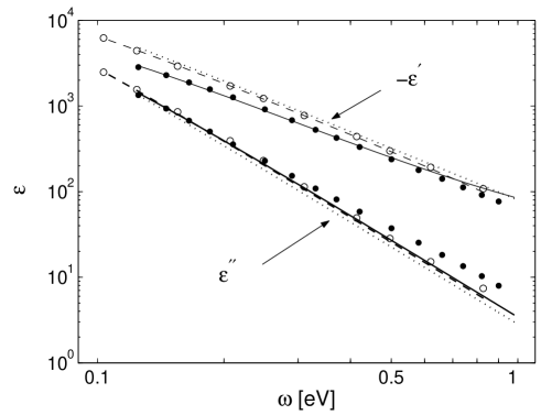
Figure 3: The infrared optical data by Dold and Mecke [29] (full circles) and by Motulevich and Shubin [40] (open circles) together with the best Drude fits given by the solid and dashed lines, respectively. The dotted lines present the fit with $\omega_{\rm p}=9$ eV and $\omega_{\tau}=35$ meV which agrees better with the Motulevich and Shubin data (open circles) than with the handbook data (full circles).

5 The Drude parameters from Kramers-Kronig analysis

Because the values of the Drude parameters are crucial for a reliable prediction of the Casimir force, it is important to assess that different methods to determine the parameters give the same results. Alternatively to the extrapolation procedure of the previous section we will now discuss a procedure based on a Kramers-Kronig analysis. To this aim we will extrapolate only the imaginary part of the dielectric function to low frequencies $\omega<\omega_{\rm c}$. The dispersion relation between $\varepsilon^{\prime}$ and $\varepsilon^{\prime\prime}$

$$\varepsilon^{\prime}(\omega)-1=\frac{2}{\pi}P\int\limits_{0}^{\infty}dx\frac{x\varepsilon^{\prime\prime}\left(x\right)}{x^{2}-\omega^{2}}$$ (13)

can then be used to predict the behavior of $\varepsilon^{\prime}(\omega)$ and compare it with the one observed in the experiments. From this comparison the Drude parameters can be extracted.

The low-frequency behavior of $\varepsilon^{\prime\prime}(\omega)$ is important for the prediction of $\varepsilon^{\prime}$ because for metals $\varepsilon^{\prime\prime}(\omega)\gg 1$ in the low frequency range. Therefore, at $\omega<\omega_{\rm c}$ we are using $\varepsilon^{\prime\prime}(\omega)$ from Eq. (9). At higher frequencies the experimental data from different sources [21, 30, 40, 41] are used. The data in Refs. [40, 41] must be extended to high frequencies starting from $\omega=1.25$ eV. We do this using the handbook data [21].

Let us start from the data for bulk Au(110) [30]. This data set is given in the interval $0.1<\omega<30$ eV. Below $\omega=0.1$ eV we use the Drude model for $\varepsilon^{\prime\prime}$ and above $\omega=30$ eV the cubic extrapolation $C/\omega^{3}$. The Drude parameters are practically insensitive to the high frequency extrapolation. The data set was divided into overlapping segments containing 12 points. Each segment was fitted with a polynomial of forth order in frequency. The first segment, were $\varepsilon^{\prime\prime}(\omega)$ increases very fast, was fitted with the polynomial in $1/\omega$. Then, in the range of overlap (4 points) a new polynomial smoothly connecting two segments was chosen. In this way we have fitted the experimental data with a function which is smooth up to the first derivative.

The real part of the dielectric function $\varepsilon^{\prime}(\omega)$ is predicted by Eq. (13) as a function of the Drude parameters $\omega_{p}$ and $\omega_{\tau}$. These parameters are chosen such as to minimize the difference between observed and predicted values of $\varepsilon^{\prime}(\omega)$, leading to $\omega_{\rm p}=8.40$ eV and $\omega_{\tau}=0.020$ eV. These parameters are in reasonable agreement with the ones indicated in Tab. 1. In Fig. 4 the experimental data (dots) and $|\varepsilon^{\prime}(\omega)|$ found from Eq. (13) (solid line) are plotted, showing perfect agreement at low frequencies, while at high frequencies $\omega>2.6$ eV the agreement is not very good. This may be fixed by choosing an appropriate high frequency extrapolation. We do not give these details here as this extrapolation has practically no influence on the Drude parameters.

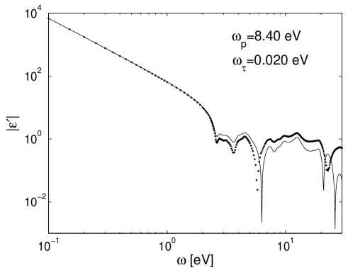
Figure 4: $|\varepsilon^{\prime}|$ as a function of $\omega$ for bulk gold. Dots are the experimental data [30]. The solid line is the prediction according to Eq. (13) with the Drude parameters $\omega_{p}=8.40\ eV$, $\omega_{\tau}=0.02\ eV$.

When applying the same procedure to the handbook data [21], we find $\omega_{p}=7.54$ eV and $\omega_{\tau}=0.051$ eV, again in agreement with the parameters indicated in Tab. 1. Fig. 5 shows a plot of $\varepsilon^{\prime}(\omega)$ predicted with these parameters. At low frequencies the agreement with the experimental data is good but it becomes worse when the interband data [29] joins the intraband (high frequency) data [28]. These two data sets correspond to samples with different optical properties. In this case the dispersion relation (13) is not necessarily very well satified. In contrast with the previous case, high frequency extrapolation cannot improve the situation; it influences the curve only marginally.

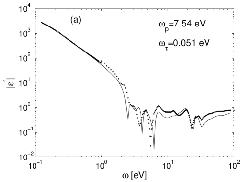
Figure 5: $|\varepsilon^{\prime}|$ as a function of $\omega$ for handbook data [21] (dots). The solid line is found from Kramers-Kronig relation. The Drude parameters correspond to minimal deviations between experimental data and calculations.

Following the same procedure for the Motulevich and Shubin data [40], we find the Drude parameters $\omega_{\rm p}=8.81$ eV, $\omega_{\tau}=0.044$ eV which are close to the values in Tab. 1. The experimental data and calculated function $|\varepsilon^{\prime}(\omega)|$ are shown in Fig. 6. There is good agreement for frequencies $\omega<4$ eV as the data in Ref. [40] matches very well the Thèye data [28]. Deviations at higher frequencies are again quite sensitive to high-frequency extrapolation as already noted before.

Similar calculations done for the Padalka and Shklyarevskii data [41] give the Drude parameters $\omega_{\rm p}=6.88$ eV and $\omega_{\tau}=0.033$ eV, producing good agreement only in the range $\omega<1.3$ eV because this data set matches only poorly the Thèye data [28].

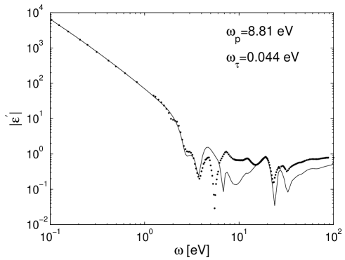
Figure 6: $|\varepsilon^{\prime}|$ as a function of $\omega$ for Motulevich and Shubin data [40] extended by the handbook data [21] for $\omega>1.25$ eV (dots). The solid line is found from Kramers-Kronig relation.

Using the Kramers-Kronig analysis for the determination of the Drude parameters leads essentially to the same parameters for all 4 sets of the experimental data. Experimental and calculated curves for $\varepsilon^{\prime}(\omega)$ are in very good agreement at low frequencies. At high frequencies the agreement is not so good for two different reasons. First, at high frequencies the calculated curve is sensitive to the high-frequency extrapolation and thus a better choice of this extrapolation can significantly reduce high frequency deviations. The other reason is that one has to combine the data from different sources to make a Kramers-Kronig analysis possible. These data sets do not always match each other well as it is for example the case of the Dold and Mecke data and the Thèye data. In this case significant errors might be introduced in the dispersion relation. Indeed the Kramers-Kronig analysis is a valuable tool only for data taken from the same sample.

6 Uncertainty in the Casimir force due to variation of optical properties

We will now assess how the values of the Casimir force are influenced by the different values of the Drude parameters. As an example we consider as input the optical data for Au from [21].

Instead of calculating the absolute value of the Casimir force, we will give the factor which measures the reduction of the Casimir force with respect to the ideal Casimir force between perfect mirrors as introduced in [18]

$$\eta_{F}=\frac{120L^{4}}{c\pi^{4}}\int\limits_{0}^{\infty}d\kappa\,\kappa^{2}\int\limits_{0}^{\kappa}d\zeta\sum_{\mu}\frac{r_{\mu}^{2}}{e^{2\kappa}-r_{\mu}^{2}},$$ (14)

The dielectric function at imaginary frequencies $\varepsilon(i\zeta)$ is calculated using the Kramers-Kronig relation (4) and the integration region is divided in two parts

$$\int_{0}^{\infty}\frac{x\,\varepsilon^{\prime\prime}(x)}{x^{2}+\omega^{2}}dx\rightarrow\left\{\int_{0}^{x_{c}}+\int_{x_{c}}^{x_{max}}\right\}\frac{x\,\varepsilon^{\prime\prime}(x)}{x^{2}+\omega^{2}}dx=I_{1}+I_{2}.$$ (15)

We assume that for $x<x_{\rm c}$ the Drude model (9) is applicable. Then the integration in $I_{1}$ may be carried out explicitly, see (8). In $I_{2}$ we integrate from $x_{\rm c}=0.125$ eV to $x_{\rm max}=9000$ eV (corresponding to the range of available optical data in [21]).

For the calculation of the reduction factor (14) the integration range was chosen as $10^{-4}-10^{3}$ eV. We also varied the integration range by half an order of magnitude, which changed the result by less than $0.1\%$. The results of the numerical integration are collected in Table 2.

	$\omega_{p},\omega_{\tau}(eV)\,\backslash L(\mu m)$	$\quad 0.1\quad$	$\quad 0.3\quad$	$\quad 0.5\quad$	$\quad 1.0\quad$	$\quad 3.0\quad$
1.	$\omega_{\rm p}=7.50$, $\omega_{\tau}=0.061$	0.43	0.66	0.75	0.85	0.93
2.	$\omega_{\rm p}=8.41$, $\omega_{\tau}=0.02$	0.45	0.69	0.79	0.88	0.95
3.	$\omega_{\rm p}=8.84$, $\omega_{\tau}=0.0422$	0.46	0.69	0.78	0.87	0.94
4.	$\omega_{\rm p}=6.85$, $\omega_{\tau}=0.0357$	0.42	0.65	0.75	0.84	0.93
5.	$\omega_{\rm p}=9.00$, $\omega_{\tau}=0.035$	0.47	0.71	0.79	0.88	0.95
6.	$\omega_{\rm p}=7.50\pm 15\%$	0.45	0.68	0.77	0.86	0.94
	$\omega_{\tau}=0.061$	0.41	0.63	0.73	0.83	0.92
7.	$\omega_{\rm p}=7.50$	0.42	0.65	0.74	0.84	0.92
	$\omega_{\tau}=0.061\pm 30\%$	0.44	0.67	0.76	0.86	0.93

Table 2: The reduction factors at different plate separations calculated with the different pairs of values of the Drude parameters corresponding to different data. The last two rows show the variation of the reduction factor when either the plasma frequency or the relaxation parameter is varied.

The first four rows of the table present the reduction factors for four pairs of the Drude parameters that were obtained by fitting the optical data from different sources. The next row shows the result obtained for $\omega_{\rm p}=9$ eV and $\omega_{\tau}=35$ meV. The last two rows show the variation of the reduction factor if the plasma frequency $\omega_{\rm p}$ or the relaxation parameter $\omega_{\tau}$ are varied by $\pm 15\%$ and $\pm 30\%$, respectively. The upper (lower) line corresponds here to the upper (lower) sign.

The variation of the optical data and the associated Drude parameters introduces a variation in the Casimir force ranging from 5.5% at short distances (100 nm) to 1.5% at long distances (3 $\mu$m). The distance dependence is of course related to the fact that the material properties influence the Casimir force much more at short than at long plate separation. The strongest variation of 5.5% gives an indication of the genuine sample dependence of the Casimir force. For this reason it is necessary to measure the optical properties of the plates used in the Casimir force measurement if a precision of the order 1% or better in the comparison between experimental values and theoretical predictions is aimed at. Incidentally let us notice that the plasma frequency $\omega_{\rm p}=7.5$ eV, which is found here to fit best Palik’s handbook data [21], is basically the same as the one proposed alternatively in [18] for Cu, which has very similar optical properties to Au concerning the Casimir force [45]. For Cu, the variation of the plasma frequency from $\omega_{\rm p}=9$ eV to $\omega_{p}=7.5$ eV introduced a variation of the Casimir force up to 5% [18].

In order to asses more quantitatively the role of the two Drude parameters, we show in the last two rows of table 2 the variation of the reduction factor when either the plasma frequency or the relaxation parameter is varied with the other parameter kept constant. One can see that the increase (decrease) of the relaxation parameter by $\delta\omega_{\tau}=30\%$ lowers (increases) the reduction factor $\eta_{F}$ at $L=0.1~{}\mu m$ by only $\delta\eta_{F}=1.6\%$. However, the $15\%$ variation of the plasma frequency leads to $4.2\%$ change in the reduction factor. Thus the Casimir force is much more sensitive to the variation of the plasma frequency, basically as the plasma frequency determines the reflection quality of the plates (an infinite plasma frequency corresponds to perfectly reflecting mirrors).

7 Conclusions

In this paper we have performed the first systematic and detailed analysis of optical data for Casmir force measurements. We have studied the relative importance of the different frequency regions for the Casimir force as a function of the plate separation and established the critical role of the Drude parameters in particular for short distance measurements. We have then analyzed and compared four different sets of optical data. For each set we have extracted the corresponding plasma frequency and relaxation parameter either by fitting real and imaginary part of the dielectric function at low frequencies or by using a detailed Kramers-Kronig analysis. Both methods lead essentially to the same results. The Kramers-Kronig analysis reveals itself to be a powerful tool for the estimation of the low frequency Drude parameters for data coming from the same sample.

A variation of the values of the Casimir force up to 5.5% is found for different optical data sets. This gives an intrinsic unknown parameter for the Casimir force calculations and demonstrates the genuine sample dependence of the Casimir force. The today existing numerical and analytical calculations of the Casimir force in themselves are very precise. In the same way, measurements of the Casimir force have achieved high accuracy over the last decade. In order to compare the results of the achievements in theory and experiment at a level of 1% precision or better, the crucial point is to make sure that calculations and experiments are performed for the same physical sample. One therefore has to know the optical and material properties of the sample used in the experiment. These properties must be measured for frequencies as low as possible. In practice, the material properties have to be known over an interval of about 4 orders of magnitude around the characteristic frequency $\zeta_{\rm ch}=c/2L$. For a plate separation of $L=100$ nm this means an interval [10 meV, 100 eV]. If measurements at low frequencies are not possible, the low frequency Drude parameters should be extracted from the measured data, by one of the two methods discussed here.

Acknowledgements Part of this work was funded by the European Contract STRP 12142 NANOCASE. We wish to thank S. Reynaud and A. Krasnoperov for useful discussions.

References

References

- [1] Casimir H B G 1948 Proc. K. Ned. Akad. Wet. 51 793.
- [2] Milonni P W 1994 The Quantum Vacuum (Academic Press, San Diego).
- [3] Mostepanenko V M and Trunov N N 1997 The Casimir Effect ans its Applications (Clarendon Press, Oxford).
- [4] Kardar M and Golestanian R 1999 Rev. Mod. Phys. 71 1233.
- [5] Milton K A 2001 The Casimir Effect (World Scientific, Singapore).
- [6] Bordag M, Mohideen U, and Mostepanenko V M 2001 Phys. Rep. 353 1.
- [7] Lamoreaux S K 1997 Phys. Rev. Lett. 78 5; 1998 81 5475.
- [8] Mohideen U and Roy A 1998 Phys. Rev. Lett. 81 4549; Roy A, Lin C-Y, and Mohideen U 1999 Phys. Rev. D 60, 111101(R).
- [9] Harris B W, Chen F, and Mohideen U 2000 Phys. Rev. A 62 052109.
- [10] Chan H B, Aksyuk V A, Kleiman R N, Bishop D J, and Capasso F 2001 Science 291 1941; 2001 Phys. Rev. Lett. 87 211801.
- [11] Decca R S, López D, Fischbach E, and Krause D E 2003 Phys. Rev. Lett. 91 050402.
- [12] Decca R S, Fischbach E, Klimchitskaya G L, Krause D E, López D, and Mostepanenko V M 2003 Phys. Rev. D 68 116003.
- [13] Decca R S, López D, Fischbach E, Klimchitskaya G L, Krause D E, and Mostepanenko V M 2005 Ann. Phys. 318 37.
- [14] Iannuzzi D, Lisanti M, and Capasso F 2004 Proc. Natinonal Acad. Sci. USA 101 4019.
- [15] Lissanti M, Iannuzzi D and Capasso F 2005 Proc. Natinonal Acad. Sci. USA 102 11989.
- [16] Bressi G, Carugno G, Onofrio R, and Ruoso G, 2002 Phys. Rev. Lett. 88 041804.
- [17] Ederth T 2000 Phys. Rev. A 62 062104.
- [18] Lambrecht A and Reynaud S 2000 Eur. Phys. J. D 8, 309.
- [19] Lifshitz E M 1956 Zh. Eksp. Teor. Fiz. 29 94 [1956 Sov. Phys. JETP 2 73].
- [20] Lifshitz E M and Pitaevskii L P 1980 Statistical Physics, Part 2 (Pergamon Press, Oxford).
- [21] Palik E D (ed) 1995 Handbook of Optical Constants of Solids (New York: Academic Press).
- [22] Svetovoy V B and Lokhanin M V 2000 Mod. Phys. Lett. A 15, 1437.
- [23] Boström M and Sernelius B E 2000 Phys. Rev. A 61 046101.
- [24] Svetovoy V B and Lokhanin M V 2000 Mod. Phys. Lett. A 15 1013.
- [25] Zolotarev V M, Morozov V N, and Smirnova E V 1984 Optical Constants of Natural and Technical Media (Khimija, Leningrad) (in Russian).
- [26] Svetovoy V B 2003 Proc. Quantum Field Theory Under External Conditions 76, Ed. Milton K A (Princeton, NJ: Rynton Press); arXiv: cond-mat/0401562.
- [27] Chen F, Klimchitskaya G L, Mohideen U, and Mostepanenko V M 2004 Phys. Rev. A 69 022117.
- [28] Thèye M-L 1970 Phys. Rev. B 2 3060.
- [29] Dold B and Mecke R 1965 Optik 22 435.
- [30] Weaver J H, Krafka C, Lynch D W, and Koch E E 1981 Optical Properties of Metals, Part II, Physics Data No. 18-2 (Fachinformationszentrum Energie, Physik, Mathematik, Karsruhe).
- [31] Sotelo J, Ederth J, and Niklasson G 2003 Phys. Rev. B 67 195106.
- [32] An I, Park M-G, Bang K-Y, Oh H-K, and Kim H 2002 Jpn. J. Appl. Phys. 41 3978.
- [33] Xia G-Q et al. 2000 Rev. Sci. Instrum. 71 2677.
- [34] Yu Wang et al. 1998 Thin Solid Films 313 232.
- [35] Bendavid A, Martin P J, Wieczorek L 1999 Thin Solid Films 354 169.
- [36] Pells G P and Shiga M 1969 J. Phys. C 2 1835.
- [37] Johnson P B and Christy R W 1972 Phys. Rev. B 6 4370.
- [38] Guerrisi M, Rosei R, and Winsemius P 1975 Phys. Rev. B 12 557.
- [39] Aspnes D E, Kinsbron E, and Bacon D D 1980 Phys. Rev. B 21 3290.
- [40] Motulevich G P and Shubin A A 1964 Zh. Eksp. Teor. Fiz. 47 840 [1965 Soviet Phys. JETP 20 560].
- [41] Padalka V G and Shklyarevskii I N 1961 Opt. Spektroskopiya 11 527 [1961 Opt. Spectry. (USSR) 11 285].
- [42] Bennett J M and Ashley E J 1965 Appl. Opt. 4 221.
- [43] Hagiwara K et al. 2002 Phys. Rev. D 66 010001.
- [44] Bennett H E and Bennett J M 1966 in Optical Properties and Electronic Structure of Metals and Alloys, edited by Abélès F (North-Holland Publ., Amsterdam).
- [45] Lambrecht A and Reynaud S 2000 Phys. Rev. Lett. 84 5672.