Deterministic Quantum Key Distribution Using Gaussian-Modulated Squeezed States

Abstract

A continuous variable ping-pong scheme, which is utilized to generate deterministically private key, is proposed. The proposed scheme is implemented physically by using Gaussian-modulated squeezed states. The deterministic way, i.e., no basis reconciliation between two parties, leads a two-times efficiency comparing to the standard quantum key distribution schemes. Especially, the separate control mode does not need in the proposed scheme so that it is simpler and more available than previous ping-pong schemes. The attacker may be detected easily through the fidelity of the transmitted signal, and may not be successful in the beam splitter attack strategy.

The standard quantum key distribution (QKD) scheme Gisin (2002) provides a novel way of generation and distribution of secret key. Its security is guaranteed by the law of quantum mechanics Lo (1999); Shor (2000); Mayers (2001). The intrinsical basis reconciliation, which is significant in guaranteeing the security, means that the standard QKD is nondeterministic. Unfortunately, the nondeterministic property results in loss of many qubits, consequently, the efficiency is very low. To improve the efficiency, several deterministic QKD schemes were proposed recently by using technique of ping-pong of photon between two parties Boström (2002); WójcikQingYu (2003); Lucamarini (2005). These schemes are implemented in discrete variable. While the final key is generated through a message-mode and the security is guaranteed by a separate control-mode. However, the separate control-mode in the previous ping-pong schemes leads a higher communication complexity and a more complicated experimental realization. In addition, discrete variable is not easy in generation as well as detection so that continuous variable (CV) becomes a favored candidate in the quantum cryptography Braunstein (2005); Ralph (1999); Hilery (2000); Gottesman (2001); Cerf (2001); Grosshans (2002); Silberhorn (2002); Grosshans (2003).

In this letter, a continuous variable ping-pong scheme, which is implemented by using the Gaussian-modulated squeezed states, is firstly proposed. Since the proposed scheme does not need the basis reconciliation when the communicators, i.e., Alice and Bob, exchange the key information, its efficiency is two times of the standard CV QKD schemes. Particularly, the separate control-mode, which is necessary in the discrete-variable (DV) ping-pong schemes, can be omitted. This characteristic makes the proposed scheme be feasible in experimental realization. In addition, the channel capacity is higher than that of the DV ping-pong schemes. The security analysis based on Shannon information theory shows clearly the security against the beam splitter attack strategy. In a lossy channel, when the transmission is larger than $0.728$ the security can be warranted.

The proposed scheme, which is sketched in Fig.1, executes the following. Step 1, Bob operates an initial vacuum state $|0\rangle$ with either operator ${\mathcal{P}}=D(\alpha)S(r)$ or ${\mathcal{P}}_{\bot}=D(i\alpha)S(-r)$ which are regarded as a pair of bases, where $S(r)$ is the squeezing operator and $r$ is the squeezed factor, $D(\alpha)$ is a displacement operator which is employed to add noise, and $\alpha$ is a real number. Step 2, Bob sends the generated state to Alice through a public quantum channel. Step 3, having operated the received state by a proper displacement operator $D(\alpha^{\prime}=x+ix)$, Alice returns the state to Bob, where $x$ is a random number which is drawn from Gaussian probability distribution. Step 4, if the base $\mathcal{P}$ is employed in the step 1, Bob applies $D(-\alpha)$ on the returned mode, and measures $X_{1}$. Otherwise, Bob applies $D(-i\alpha)$ on the returned mode, and measures $X_{2}$. The canonical quadratures $X_{1}$ and $X_{2}$ are defined as $X_{1}=\frac{1}{2}(\hat{a}+\hat{a}^{{\dagger}})$ and $X_{2}=\frac{1}{2i}(\hat{a}-\hat{a}^{{\dagger}})$. Step 5, Alice randomly selects some $x$ values, and then sends the chosen values and their corresponding time slots to Bob through a public classic channel. Step 6, after has received Alice’s values, Bob calculates statistically the fidelity by using the received values and his corresponding measured results. Then Bob detects whether Eve is absent or not by using the calculated fidelity.

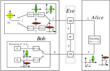
Figure 1: Scheme of the deterministic quantum key distribution using Gaussian-modulated squeezed states. The Arabian numbers denote the modes in Heisenburg picture.

We explain briefly above protocol in the physical way. Bob’s operation in step 1 yields a squeezed coherent state either $|\alpha,r\rangle=D(\alpha)S(r)|0\rangle$ or $|i\alpha,-r\rangle=D(i\alpha)S(-r)|0\rangle$. For simplicity, we only illuminate the evolvement of the state $|\alpha,r\rangle$ thereafter since the state $|i\alpha,-r\rangle$ may be treated with in a same way. Since the initial vacuum state $|0\rangle$ is a Gaussian state, the canonical quadratures $X^{1}_{1}$ and $X^{1}_{2}$ follow the Gaussian probability distribution, i.e., $X_{1}^{1}\sim N(0,\frac{1}{4})$ and $X_{2}^{1}\sim N(0,\frac{1}{4})$, where $X^{i}_{k}(k=1,2)$ represents $X_{k}(k=1,2)$ of the mode $\hat{a}_{i}$, $\Gamma\sim N(\mu,\sigma^{2})$ denotes that random variable $\Gamma$ follows Gaussian probability distribution with the average value $\mu$ and the variance $\sigma^{2}$. Choosing a random disturbance $\alpha$ with distribution $A\sim N(0,\Sigma^{2})$, one has $X_{1}^{3}\sim N(0,\Sigma^{2}+\frac{1}{4}e^{-2r})$ and $X_{2}^{3}\sim N(0,\frac{1}{4}e^{2r})$. Obviously, when the following condition is satisfied, i.e.,

$$\Sigma^{2}+\frac{1}{4}e^{-2r}=\frac{1}{4}e^{2r},$$ (1)

$X_{1}^{3}$ and $X_{2}^{3}$ follows the same probability distribution. Subsequently, Eve cannot distinguish the output states $|\alpha,r\rangle$ and $|i\alpha,-r\rangle$ whatever the statistics Eve accumulates. Making use of the operator $D(\alpha^{\prime}=x+ix)$ and the distribution $X\sim N(0,\Sigma{{}^{\prime}}^{2})$, one may easily obtain $X_{1}^{5}\sim N(0,\Sigma^{2}+\frac{1}{4}e^{-2r}+{\Sigma^{{}^{\prime}}}^{2})$ and $X_{2}^{5}\sim N(0,\frac{1}{4}e^{2r}+{\Sigma^{{}^{\prime}}}^{2})$. After has received the state encoded by Alice, Bob removes the added quantum noise so that he can decode Alice’s message. This operation gives the mode $\hat{a}_{7}$ with $X_{1}^{7}\sim N(0,\frac{1}{4}e^{-2r}+{\Sigma^{{}^{\prime}}}^{2})$ and $X_{2}^{7}\sim N(0,\frac{1}{4}e^{2r}+{\Sigma^{{}^{\prime}}}^{2})$. Finally, Bob measures $X_{1}^{7}$ on the received state to decode Alice’s message.

Now we move on the security analysis. Suppose Eve splits the forward and backward beams as depicted in Fig.1, then she coherently measures the intercepted beams to obtain the maximal information. To show the security of the proposed scheme against above attack strategy, i.e., the general beam splitter attack strategy, we adopt the following criterion which is used prevalently for QKD scheme Gisin (2002); Maurer (1993),

$$\Delta I=I(\alpha,\beta)-I_{max}(\alpha,\epsilon)>0,$$ (2)

where $I(\alpha,\beta)$ is the mutual information between Alice and Bob, and $I_{max}(\alpha,\epsilon)$ is the maximal mutual information between Alice and Eve. According to Shannon information theory Shannon (1948), the channel capacity of the additive white Gaussian noise (AWGN) channel is given by,

$$I=\frac{1}{2}\log_{2}(1+\gamma),$$ (3)

where $\gamma=P_{S}/P_{N}$ is the signal-noise ratio, $P_{S}$ and $P_{N}$ are the variances of the signal and noise probability distributions respectively. If the signal follows the Gaussian distribution, and the channel is an AWGN channel, the channel capacity is the mutual information of the communication parties. In the followings, first we calculate the probability distributions of $X_{1}$ and $X_{2}$ in all modes as depicted in Fig.1, then calculate $I(\alpha,\beta)$ and $I_{max}(\alpha,\epsilon)$ according to Eq.(3).

A beam splitter (BS) is always employed to split the laser beam. According to Fig.1, inputs of the $BS_{1}$ are given by,

$$X_{1}^{3}=e^{-r}X_{1}^{1}+A,\,\,\,X_{2}^{3}=e^{r}X_{2}^{1}.$$ (4)

and two output modes of $BS_{1}$ are,

$$X_{1}^{4}=\sqrt{\eta_{1}}X_{1}^{3}+\sqrt{1-\eta_{1}}X_{1}^{vac1},$$

$$X_{2}^{4}=\sqrt{\eta_{1}}X_{2}^{3}+\sqrt{1-\eta_{1}}X_{2}^{vac1},$$

$$X_{1}^{8}=\sqrt{\eta_{1}}X_{1}^{vac1}-\sqrt{1-\eta_{1}}X_{1}^{3},$$

$$X_{2}^{8}=\sqrt{\eta_{1}}X_{2}^{vac1}-\sqrt{1-\eta_{1}}X_{2}^{3},$$ (5)

where ${\eta_{1}}$ is the transmittance coefficient of $BS_{1}$. Consider Alice’s operation of applying the displacement operator $D(\alpha^{{}^{\prime}}=x+ix)$ on the mode $\hat{a}_{4}$, the inputs of the $BS_{2}$ are given by,

$$X_{1}^{5}=X_{1}^{4}+X,\,\,\,X_{2}^{5}=X_{2}^{4}+X.$$ (6)

Similarly, the outputs of the $BS_{2}$ are obtained as following,

$$X_{1}^{6}=\sqrt{\eta_{2}}X_{1}^{5}+\sqrt{1-\eta_{2}}X_{1}^{vac2},$$

$$X_{2}^{6}=\sqrt{\eta_{2}}X_{2}^{5}+\sqrt{1-\eta_{2}}X_{2}^{vac2},$$

$$X_{1}^{9}=\sqrt{\eta_{2}}X_{1}^{vac2}-\sqrt{1-\eta_{2}}X_{1}^{5},$$

$$X_{2}^{9}=\sqrt{\eta_{2}}X_{2}^{vac2}-\sqrt{1-\eta_{2}}X_{2}^{5},$$ (7)

where ${\eta_{2}}$ is the transmittance coefficient of $BS_{2}$. Applying the operator $D(-\alpha)$ on mode $\hat{a}_{6}$ yields,

$$X_{1}^{7}=X_{1}^{6}-A,\,\,\,\,\,\,X_{2}^{7}=X_{2}^{6}.$$ (8)

Combining Eqs.(4) $\sim$ (8) gives,

$$X_{1}^{7} = \sqrt{\eta_{2}}[\sqrt{\eta_{1}}(e^{-r}X_{1}^{1}+A)+\sqrt{1-\eta_{1}}X_{1}^{vac1}+X]+\sqrt{1-\eta_{2}}X_{1}^{vac2}-A,$$

$$X_{2}^{7} = \sqrt{\eta_{2}}(\sqrt{\eta_{1}}e^{r}X_{2}^{1}+\sqrt{1-\eta_{1}}X_{2}^{vac1}+X)+\sqrt{1-\eta_{2}}X_{2}^{vac2},$$ (9)

where the random variables $X_{k}^{j}$ ($k=1,2,j=vac1,vac2$) follow the Gaussian probability distributions, i.e.,

$$X_{k}^{j}\sim N(0,\frac{1}{4}).$$ (10)

Making use of Eqs.(1), (Deterministic Quantum Key Distribution Using Gaussian-Modulated Squeezed States) and (10), the variances of $X_{1}^{7}$ and $X_{2}^{7}$ are obtained,

$$\langle(\Delta X_{1}^{7})^{2}\rangle = \frac{1}{4}\eta_{1}\eta_{2}e^{-2r}+\frac{1}{4}(1-\sqrt{\eta_{1}\eta_{2}})^{2}(e^{2r}-e^{-2r})$$ (11)

$$+\eta_{2}\Sigma^{{}^{\prime}2}+\frac{1}{4}[(1-\eta_{2})+(1-\eta_{1})\eta_{2}],$$

$$\langle(\Delta X_{2}^{7})^{2}\rangle = \frac{1}{4}\eta_{1}\eta_{2}e^{2r}+\eta_{2}\Sigma^{{}^{\prime}2}+\frac{1}{4}[(1-\eta_{2})+(1-\eta_{1})\eta_{2}].$$

Using the first expression in Eq.(11) gives the signal-noise ratio,

$$\gamma_{\alpha\beta}=\frac{M}{N}.$$ (12)

where $M=\eta_{2}\Sigma^{{}^{\prime}2}$ and $N=\frac{1}{4}\eta_{1}\eta_{2}e^{-2r}+\frac{1}{4}(1-\sqrt{\eta_{1}\eta_{2}})^{2}(e^{2r}-e^{-2r})+\frac{1}{4}[(1-\eta_{2})+(1-\eta_{1})\eta_{2}]$. Thus the mutual information between Alice and Bob is,

$$I(\alpha,\beta)=\frac{1}{2}\log_{2}(1+\gamma_{\alpha\beta}).$$ (13)

When $\eta_{1}=\eta_{2}=1$, above equation can be written as $C(\alpha,\beta)=\frac{1}{2}\log_{2}(1+\frac{4\Sigma^{{}^{\prime}2}}{e^{-2r}})$, where $C(\alpha,\beta)$ is the mutual information between Alice and Bob without eavesdropping. Obviously, $C(\alpha,\beta)$ increases with $r$ and $\Sigma^{{}^{\prime}2}$. Actually, $C(\alpha,\beta)$ is the channel capacity of the communication between Alice and Bob without eavesdropping. As an example, one may easily obtain $C(\alpha,\beta)=8.6$ bits when $r=3,\Sigma^{\prime}=10$, which is apparently larger than that of the DV quantum communication scheme.

The maximal information $I_{max}(\alpha,\epsilon)$ may be obtained by Eve through measuring both $\hat{a}_{8}$ and $\hat{a}_{9}$. Assume that Eve is an evil quantum physicist who is able to build all devices that are allowed by the laws of quantum mechanics. Then Eve may build an advice to measure $X_{1}^{Eve}$ and $X_{2}^{Eve}$ of the mode $\hat{a}_{Eve}=\hat{a}_{9}-k\hat{a}_{8}$, where $k$ is a parameter to be optimized. Using the expressions of $X^{8}_{k}$ in Eq.(Deterministic Quantum Key Distribution Using Gaussian-Modulated Squeezed States) and $X^{9}_{k}$ in Eq.(Deterministic Quantum Key Distribution Using Gaussian-Modulated Squeezed States), $X_{1}^{Eve}$ and $X_{2}^{Eve}$ may be easily obtained,

$$X_{1}^{Eve} = -[\sqrt{\eta_{1}(1-\eta_{2})}-k\sqrt{1-\eta_{1}}](e^{-r}X_{1}^{1}+A)-$$ (14)

$$\sqrt{1-\eta_{2}}X-[\sqrt{(1-\eta_{1})(1-\eta_{2})}+k\sqrt{\eta_{1}}]X_{1}^{vac1}+\sqrt{\eta_{2}}X_{1}^{vac2},$$

$$X_{2}^{Eve} = -[\sqrt{\eta_{1}(1-\eta_{2})}-k\sqrt{1-\eta_{1}}]e^{r}X_{2}^{1}-\sqrt{1-\eta_{2}}X-$$

$$[\sqrt{(1-\eta_{1})(1-\eta_{2})}+k\sqrt{\eta_{1}}]X_{2}^{vac1}+\sqrt{\eta_{2}}X_{2}^{vac2}.$$

Combining Eq.(1) and Eq.(14), one may find that the random variables $X_{1}^{Eve}$ and $X_{2}^{Eve}$ follow the same probability distribution. Accordingly, Eve obtains the same signal-noise ratios in $X_{1}^{Eve}$ and $X_{2}^{Eve}$, i.e., $\gamma_{\alpha\epsilon X_{1}^{Eve}}=\gamma_{\alpha\epsilon X_{2}^{Eve}}={4(1-\eta_{2})\Sigma^{{}^{\prime}2}}/{\mu+\nu}$, where $\mu=(\sqrt{\eta_{1}(1-\eta_{2})}-k\sqrt{1-\eta_{1}})^{2}e^{2r}$ and $\nu=(\sqrt{(1-\eta_{1})(1-\eta_{2})}+k\sqrt{\eta_{1}})^{2}+\eta_{2}$. When $k=(e^{2r}+1)\sqrt{\eta_{1}(1-\eta_{1})(1-\eta_{2})}/(e^{2r}(1-\eta_{1})+\eta_{1})$, Eve obtains the maximal mutual information,

$$I_{max}(\alpha,\epsilon) = I_{X_{1}}(\alpha,\epsilon)=I_{X_{2}}(\alpha,\epsilon).$$ (15)

Substituting Eqs.(13) and (15) into Eq.(2) gives the secret information rate $\Delta I$. Fig.2 shows the properties of $\Delta I$ changing with $\eta_{1},\eta_{2}$. One may see that $\Delta I$ increases with increasing of $\eta_{1},\eta_{2}$. In addition, $\Delta I$ may be negative when $\eta_{1}$ and $\eta_{2}$ are small, which implicates that Eve may obtain more useful information by choosing two proper beam splitters than Bob. Fortunately, this attack strategy does not influence the security of the proposed scheme since Eve may be detected easily in this situation.

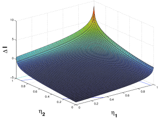
Figure 2: Property of $\Delta I$ (unit:bit) changing with $\eta_{1},\eta_{2}$. The employed parameters are $r=3$ and $\Sigma^{{}^{\prime}2}=100$.

Now we investigate how to detect Eve. A separate control-mode is always employed to detect the eavesdropping in the previous ping-pong schemes. However, this approach does not benefit the efficiency of the scheme. Here we propose a new approach which is more efficient than the separate control-mode approach. After finished the step 4, Alice tells Bob some values of random variable $X$ and the corresponding time slots through a classical public channel. After received Alice’s results, Bob calculates the fidelity,

$$F=\langle\alpha_{in}|\rho_{out}|\alpha_{in}\rangle=\pi Q(\alpha_{in}),$$ (16)

where $|\alpha_{in}\rangle=|0\rangle$, $\rho_{out}=|\alpha_{out}\rangle\langle\alpha_{out}|$, and $|\alpha_{out}\rangle=S(-r)D(-\alpha^{{}^{\prime}})|\Psi\rangle$ with the quantum state $|\Psi\rangle$ in mode $\hat{a}_{7}$. The $Q$ function for a squeezed state is defined as that in qoptics (1994). In an ideal (no-loss) quantum channel, the fidelity satisfies $F=1$ without eavesdropping and $F<1$ with eavesdropping. Therefore the fidelity $F$ can be employed as an important parameter for Eve detection. Making use of the state $|\alpha_{out}\rangle$ in the Heisenburg picture and Eq.(Deterministic Quantum Key Distribution Using Gaussian-Modulated Squeezed States), one obtains,

$$X_{1}^{out} = e^{r}\{\sqrt{\eta_{2}}[\sqrt{\eta_{1}}(e^{-r}X_{1}^{1}+A)+\sqrt{1-\eta_{1}}X_{1}^{vac1}+X]+\sqrt{1-\eta_{2}}X_{1}^{vac2}-A-X\}$$

$$X_{2}^{out} = e^{-r}[\sqrt{\eta_{2}}(\sqrt{\eta_{1}}e^{r}X_{2}^{1}+\sqrt{1-\eta_{1}}X_{2}^{vac1}+X)+\sqrt{1-\eta_{2}}X_{2}^{vac2}-X].$$ (17)

Using Eqs.(10) and (17), the variances of $X_{1}^{out}$ and $X_{2}^{out}$ are given by,

$$\langle(\Delta X_{1}^{out})^{2}\rangle = e^{2r}\{\frac{1}{4}\eta_{1}\eta_{2}e^{-2r}+(1-\sqrt{\eta_{1}\eta_{2}})^{2}\Sigma^{2}$$

$$+ (\sqrt{\eta_{2}}-1)^{2}\Sigma^{{}^{\prime}2}+\frac{1}{4}[(1-\eta_{2})+(1-\eta_{1})\eta_{2}]\},$$

$$\langle(\Delta X_{2}^{out})^{2}\rangle = e^{-2r}\{\frac{1}{4}\eta_{1}\eta_{2}e^{2r}+(\sqrt{\eta}_{2}-1)^{2}\Sigma^{{}^{\prime}2}$$ (18)

$$+ \frac{1}{4}[(1-\eta_{2})+(1-\eta_{1})\eta_{2}]\}.$$

The fidelity $F$ is obtained as the following form,

$$F=\frac{2}{\sqrt{(4\langle(\Delta X_{1}^{out})^{2}\rangle+1)(4\langle(\Delta X_{2}^{out})^{2}\rangle+1)}}.$$ (19)

Substituting Eq.(Deterministic Quantum Key Distribution Using Gaussian-Modulated Squeezed States) into Eq.(19), one may calculate the fidelity. Numerical solutions of Eq.(19) are depicted in Fig.3. With $\eta_{1}$ and $\eta_{2}$ decreasing the fidelity $F$ decreases rapidly. Accordingly, any eavesdropping can be detected by Alice and Bob by using the fidelity $F$.

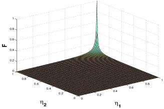
Figure 3: The dependence of fidelity $F$ on $\eta_{1}$ and $\eta_{2}$, the chosen parameters are $r=3$ and $\Sigma^{{}^{\prime}2}=100$.

The relationship between $\Delta I_{min}$ and $F$ is useful for detecting eavesdropping. The analytical expression for these variables is very prolix, so only the numerical solutions, which are plotted in Fig.4, are presented. If Eve doesn’t exist, i.e., $F=1$, one may easily obtain the secret information rate $\Delta I_{min}=I(\alpha,\beta)=8.6$ bits. However, the condition of $F=1$ is too strict in practices. Fortunately, there is an important value $F_{c}$ which may be obtained from Fig.4, i.e., $F_{c}=0.02$. When $F>F_{c}$ one has $\Delta I_{min}>0$, which means Eve’s eavesdropping does not influence the security of the final key. While $F<F_{c}$ there is a negative information rate. In this case, Alice and Bob has to discard the communication.

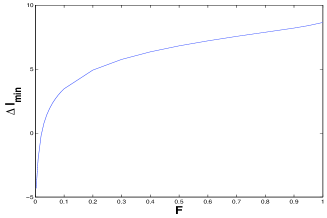
Figure 4: The relationship between $\Delta I_{min}$ (unit:bit) and $F$. The parameters are $r=3$ and $\Sigma^{{}^{\prime}2}=100$.

When the line has a transmission $\eta$ over the separation between Alice and Bob, the best attack strategy for Eve is to take a fraction $1-\eta$ of the beam and then send the fraction $\eta$ forward through her own lossless line. In this situation, the eavesdropping can not be detected but the secure QKD is possible under a proper condition. Eve’s maximum information is given by Eq.(15) with $\eta_{1}=\eta_{2}=\eta$. Numerical calculation shows $\Delta I\geq 0$ when $\eta\geq 0.728$. Accordingly, Alice and Bob can perform a deterministic QKD with security when the line has a transmission $\eta\geq 0.728$. One may recall that the coherent state quantum key distribution beats the loss limit $\eta=0.5$ by applying technique of reverse reconciliation Grosshans (2003) or postselection Siberhor (2002). Actually, with the technique of the reverse reconciliation or the postselection, the loss limit $\eta=0.728$ is anticipated to be beaten in the proposed scheme Detail (2005).

In conclusion, a deterministic QKD scheme using Gaussian-modulated squeezed states is proposed. The characteristic of no basis reconciliation yields a two-times efficiency than that of the CV standard QKD schemes. Especially, the separate control-mode does not need in the proposed scheme so that the scheme is more feasible in experimental realization. The fidelity is employed to detect the eavesdropper and resist the beam splitter attack strategy. In a lossy channel, a secure scheme requires the transmission of $\eta>0.728$.

This work is supported by the Natural Science Foundation of China, Grant No. 60472018. GQH acknowledge fruitful discussions with prof. Z.M.Zhang.

References

Gisin (2002)
N. Gisin, G. Ribordy, W. Tittel, and H. Zbinden, Rev. Mod. Phys. 74, 145 (2002), and
references therein.
Lo (1999)
H. K. Lo and H. F. Chau, Science 283, 2050 (1999).
Shor (2000)
P. W. Shor and J. Preskill, Phy. Rev. Lett. 85, 441 (2000).
Mayers (2001)
D. Mayers, Journal of the ACM 48, 351 (2001).
Boström (2002)
K. Boström and T. Felbinger, Phy. Rev. Lett. 89, 187902 (2002).
WójcikQingYu (2003)
A. Wójcik, Phy. Rew. Lett. 90, 157901 (2003).
Lucamarini (2005)
M. Lucamarini and S. Mancini, Phy. Rew. Lett. 94, 140501 (2005).
Braunstein (2005)
S. L. Braunstein and P. v. Loock, Rev. Mod. Phy. 77, 513 (2005), and reference therein.
Ralph (1999)
T. C. Ralph, Phy. Rev. A 61, 010303 (1999).
Hilery (2000)
M. Hilery, Phy. Rev. A 61, 022309 (2000).
Gottesman (2001)
D. Gottesman and J. Preskill, Phy. Rev. A 63, 022309 (2001).
Cerf (2001)
N. J. Cerf, M. Lévy, and G. V. Assche, Phy. Rev. A 63, 052311 (2001).
Grosshans (2002)
F. Grosshans and P. Grangier, Phy. Rev. Lett. 88, 057902 (2002).
Silberhorn (2002)
Ch. Silberhorn, N. Korolkova, and G. Leuchs, Phy. Rev. Lett. 88, 167902 (2002).
Grosshans (2003)
F. Grosshans et al., Nature(London) 421, 238 (2003).
Maurer (1993)
U. M. Maurer, IEEE Trans. Inf. Theory 39, 733 (1993).
Shannon (1948)
C. E. Shannon, Bell. Syst. Tech. J. 27, 623 (1948).
qoptics (1994)
D. F. Walls and G. J. Milburn, Quantum Optics. (Springer-Verlag Press, New York, 1997).
Siberhor (2002)
Ch. Silberhorn, T. C. Ralph, N. Lütkenhaus, and G. Leuchs,
Phy. Rev. Lett. 89, 167901 (2002).
Detail (2005)
Detailed calculations will be presented elsewhere for space
reasons.