Infinite Correlation in Measured Quantum Processes

Abstract

We show that quantum dynamical systems can exhibit infinite correlations in their behavior when repeatedly measured. We model quantum processes using quantum finite-state generators and take the stochastic language they generate as a representation of their behavior. We analyze two spin-$1$ quantum systems that differ only in how they are observed. The corresponding language generated has short-range correlation in one case and infinite correlation in the other.

We study how sequences produced by a quantum information source can produce infinite-length correlations. To start, we recall the finitary quantum generators defined in Ref. [1]. They consist of a finite set of internal states $Q=\{q_{i}:i=1,\ldots,|Q|\}$. The state vector is an element of a $|Q|$-dimensional Hilbert space: $\mathinner{\langle{\psi}|}\in\mathcal{H}$. At each time step a quantum generator outputs a symbol $s\in{\mathcal{A}}$ and updates its state vector as follows.

The temporal dynamics is governed by a set of $|Q|$-dimensional transition matrices $\{T(s)=U\cdot P(s),s\in{\mathcal{A}}\}$, whose components are elements of the complex unit disk and where each is a product of a unitary matrix $U$ and a projection operator $P(s)$. $U$ is a $|Q|$-dimensional unitary evolution operator that governs the evolution of the state vector. $\mathbf{P}=\{P(s):s\in{\mathcal{A}}\}$ is a set of projection operators—$|Q|$-dimensional Hermitian matrices—that determines how the state vector is measured.

The output symbol $s$ is identified with the measurement outcome and labels the system’s eigenstates. The projection operators determine how output symbols are generated from the internal, hidden unitary dynamics. They are the only way to observe a quantum process’s current internal state.

We can now describe a quantum generator’s operation. $U_{ij}$ gives the transition amplitude from internal state $q_{i}$ to internal state $q_{j}$. Starting in state vector $\mathinner{\langle{\psi_{0}}|}$ the generator updates its state by applying the unitary matrix $U$. Then the state vector is projected using $P(s)$ and renormalized. Finally, symbol $s\in{\mathcal{A}}$ is emitted. In other words, starting with state vector $\mathinner{\langle{{\psi_{0}}}|}$, a single time-step yields $\mathinner{\langle{\psi(s)}|}=\mathinner{\langle{\psi_{0}}|}U\cdot P(s)$.

An observer is interested in what can be observed and these are the measurement outcomes $s\in{\mathcal{A}}$. Thus, the only way to describe a quantum process is in terms of the sequence $\stackrel{{\scriptstyle\leftrightarrow}}{{S}}\,\equiv\,\ldots S_{-2}S_{-1}S_{0}S_{1}\ldots$ of observed random variables $S_{t}$ produced by a quantum generator. We consider a family of distributions, $\{{\rm Pr}(s_{t+1},\ldots,s_{t+L}):s_{t}\in{\mathcal{A}}\}$, where ${\rm Pr}(s_{t})$ denotes the probability that at time $t$ the random variable $S_{t}$ takes on the particular value $s_{t}\in{\mathcal{A}}$ and ${\rm Pr}(s_{t+1},\ldots,s_{t+L})$ denotes the joint probability over sequences of $L$ consecutive measurement outcomes. We assume that the distribution is stationary; ${\rm Pr}(S_{t+1},\ldots,S_{t+L})={\rm Pr}(S_{1},\ldots,S_{L})$. We denote a block of $L$ consecutive variables by $S^{L}\equiv S_{1}\ldots S_{L}$ and the lowercase $s^{L}=s_{1}s_{2}\cdots s_{L}$ denotes a particular measurement sequence of length $L$. We use the term quantum process to refer to the joint distribution ${\rm Pr}(\stackrel{{\scriptstyle\leftrightarrow}}{{S}})$ over the infinite chain of random variables. A quantum process, defined in this way, is the quantum analog of what Shannon referred to as an information source [2]. We can now determine word probabilities of observations of a quantum finite-state generator (QFG). Starting the generator in $\mathinner{\langle{\psi_{0}}|}$ the probability of output symbol $s$ is given by the state vector without renormalization:

$$\mathrm{Pr}(s)=\mathinner{\langle{\psi(s)|\psi(s)}\rangle}~{}.$$ (1)

The probability of outcomes $s^{L}$ from a measurement sequence is

$$\mathrm{Pr}(s^{L})=\mathinner{\langle{\psi(s^{L})|\psi(s^{L})}\rangle}~{}.$$ (2)

We will now investigate word probabilities of a particular quantum process. Consider a spin-$1$ particle that is subject to a magnetic field which rotates the spin. The state evolution can be described by the following unitary matrix:

$$U=\left(\begin{array}[]{ccc}\frac{1}{\sqrt{2}}&\frac{1}{\sqrt{2}}&0\\ 0&0&-1\\ -\frac{1}{\sqrt{2}}&\frac{1}{\sqrt{2}}&0\end{array}\right)~{}.\\$$ (3)

Geometrically, $U$ defines a rotation in $R^{3}$ around the y-axis by angle $\frac{\pi}{4}$ followed by a rotation around the x-axis by an angle $\frac{\pi}{2}$.

Using a suitable representation of the spin operators $J_{i}$ [3] such as:

$$J_{x} =\left(\begin{array}[]{ccc}0&0&0\\ 0&0&i\\ 0&-i&0\end{array}\right),~{}J_{y}=\left(\begin{array}[]{ccc}0&0&i\\ 0&0&0\\ -i&0&0\end{array}\right),~{}$$ (10)

$$J_{z} =\left(\begin{array}[]{ccc}0&i&0\\ -i&0&0\\ 0&0&0\end{array}\right),$$ (14)

the relation $P_{i}=1-J_{i}^{2}$ defines a one-to-one correspondence between the projector $P_{i}$ and the square of the spin component along the i-axis. The resulting measurement represents the yes-no question, Is the square of the spin component along the $i$-axis zero?

Consider the observable $J_{y}^{2}$. Then the following projection operators define the quantum finite-state generator:

$$P(0)=\mathinner{|{010}\rangle}\mathinner{\langle{010}|}~{}\mathrm{and}~{}~{}P(1)=\mathinner{|{101}\rangle}\mathinner{\langle{101}|}~{}.$$ (15)

The stochastic language generated by this process is the so-called Golden-Mean Process language [4]. It is defined by the set of irreducible forbidden words $\mathcal{F}=\{00\}$. That is, no consecutive zeros occur. For the spin-$1$ particle this means that the spin component along the y-axis never equals 0 twice in a row. We call this short-range correlation since there is a correlation between a measurement outcome at time $t$ and the immediately preceding one at time $t-1$. If the outcome is $0$ the next outcome will be $1$ with certainty. If the outcome is $1$ the next measurement is maximally uncertain: outcomes $0$ and $1$ occur with equal probability.

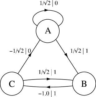
Figure 1: The Even Process quantum generator.

Figure 2: Even Process stochastic language: Words $\{01^{2k-1}0\},k=1,2,3,...$ have zero probability; all others have nonzero probability. The logarithm base 2 of the word probabilities is plotted versus the binary string $s^{L}$, represented as base-$2$ real number “$0.s^{L}$”. To allow word probabilities to be compared at different lengths, the distribution is normalized on $[0,1]$—that is, the probabilities are calculated as densities.

Consider the same Hamiltonian, but now use instead the observable $J_{x}^{2}$. The corresponding projection operators define the QFG:

$$P(0)=\mathinner{|{100}\rangle}\mathinner{\langle{100}|}~{}\mathrm{and}~{}~{}P(1)=\mathinner{|{011}\rangle}\mathinner{\langle{011}|}~{}.$$ (16)

The QFG defined by $U$ and the above projection operators is shown in Fig. 1. The stochastic language generated by this process is the so-called Even Process language [4]. The word distribution is shown in Fig. 2. It is defined by the infinite set of irreducible forbidden words $\mathcal{F}=\{01^{2k-1}0\},k=1,2,3,...$. That is, if the spin component equals 0 along the y-axis it will be zero an even number of consecutive measurements before being observed to be nonzero. This is where the infinite correlation is found: For a possibly infinite number of time steps the system tracks the evenness or oddness of number of consecutive measurements of “spin component equals 0 along the y-axis”.

The above examples show that quantum dynamical systems store information in their behavior. The quantum Even Process example is particularly striking since it has only three internal states, but exhibits infinitely long temporal correlations. Comparing the two examples demonstrates, in addition, that the amount of stored information depends on the means taken to observe the system. These properties are quantified by adapting information-theoretic measures of randomness and memory to quantum processes. We demonstrated that a repeatedly measured quantum dynamical system can store, in its current state, information about previous measurement outcomes.

In quantum computation the experimentalist subjects information stored in an initially coherent set of physical degrees of freedom to a selected sequence of manipulations. The system’s resulting state is measured and interpreted as the output of a computation. Our computation-theoretic approach, in contrast, applies to continuous computation and shows how information processing is embedded in even simple quantum systems’ behavior.

References

- [1] K. Wiesner and J. P. Crutchfield. Computation in finitary quantum processes. 2006. e-print arxiv/quant-ph/0608206.
- [2] T. Cover and J. Thomas. Elements of Information Theory. Wiley-Interscience, 1991.
- [3] Albert Messiah. Quantum Mechanics, volume II. John Wiley & Sons, Inc. – New York, 1962.
- [4] J. P. Crutchfield and D. P. Feldman. Regularities unseen, randomness observed: Levels of entropy convergence. Chaos, 13:25 – 54, 2003.
- [5] K. Wiesner and J. P. Crutchfield. Language diversity in measured quantum processes. Intl. J. Unconventional Computation, 2006. in press.