Nonlocal field correlations and dynamical Casimir-Polder forces between one excited- and two ground-state atoms

Abstract

The problem of nonlocality in the dynamical three-body Casimir-Polder interaction between an initially excited and two ground-state atoms is considered. It is shown that the nonlocal spatial correlations of the field emitted by the excited atom during the initial part of its spontaneous decay may become manifest in the three-body interaction. The observability of this new phenomenon is discussed.

I Introduction

The existence of observable effects originating from the quantum nature of the electromagnetic field has received much attention since 1948 when Casimir predicted that zero-point field fluctuations give rise to an attractive force between two neutral conducting plates at rest in the vacuum C48 . The same year Casimir and Polder provided an explanation for the retarded long-range van der Waals interaction between two neutral polarizable objects as a manifestation of the zero-point energy of the electromagnetic field CP48 . They found that retardation yields a decay law of the interaction energy as $r^{-7}$ at large interatomic separation (Casimir-Polder potential). Casimir’s results also showed how geometrical constraints can affect vacuum field fluctuations. These effects have been measured experimentally, and the results obtained are in good agreement with the theory SBCSH93 ; Lamoreaux97 ; BMM01 . More recently the attention of theoreticians has been also drawn by how a dynamical change of geometrical or topological boundaries affects vacuum field fluctuations, giving rise to observable effects such as modifications of the Casimir effect ILC04 or creation of real quanta from the vacuum (the so-called dynamical Casimir effect) FD76 ; KG99 . Dynamical Casimir effect is closely related to the Unruh effect, which establishes that an atom or a charge uniformly accelerated in the vacuum behaves as if it were immersed in a bath of thermal radiation with a temperature proportional to its acceleration U76 . The concept underlying all these phenomena is that the notion of vacuum and its physical properties depend critically on the physical system considered and on the boundary conditions.

Initially, the interatomic Casimir-Polder (CP) potential was understood in terms of the energy of the zero-point fluctuations of the electromagnetic field. More recently, it was shown that it can be also obtained as a consequence of the existence of correlations between the fluctuating dipole moments of the atoms, induced by the spatially correlated vacuum fluctuations. In other words, the CP interaction energy between two atoms in their ground state can be seen as the classical interaction energy between the instantaneous atomic dipoles, induced and correlated by the spatially-correlated vacuum field fluctuations PT93 ; PPR03a . This model is conceptually intriguing because gives a classical picture of CP forces: the quantum nature of the electromagnetic field enters only in the assumption of vacuum fluctuations as a “real” field affecting atomic dynamics. This model has been also generalized to the three-body CP potential between three atoms in their ground or excited states CP97 ; PPR05 . In this case, any pair of atoms interacts via their dipole moments which are induced and correlated by the vacuum field fluctuations, modified (dressed) by the presence of the third atom. Because the presence of one atom modifies the spatial correlations of the electric field, the interaction between two atoms changes if a third atom is present, and this evantually yields a non-additive interaction. Thus CP forces between atoms are a direct manifestation of the existence of nonlocal correlation of zero-point fluctuations, and so their measure can be used as an indirect evidence of field correlations and for investigating their nonlocal properties.

Many conceptual difficulties in quantum mechanics are involved in the notion of nonlocal correlations, also in connection with relativistic causality. In particular, Hegerfeldt reopened the question of nonlocality and causality in the QED context on a quite general basis H94 ; MJF95 ; PT97 ; PPO00 ; POP01 ; AKP01 ; CPPP03 . Specific calculations have shown that the dynamics of local atomic or field operators is causal, but that the correlation of atomic excitations of two spatially separated atoms exhibits a nonlocal behaviour, being different from zero even if the two atomic sites have a spacelike separation BCPPP90 ; PT97 . Non-local terms appear also in the spatial correlations of the energy density during the dynamical dressing/undressing of a static source interacting with the relativistic scalar field LP95 . The question of relativistic causality and its relation with the nonlocal correlations of vacuum fluctuations has been also examined in connection with the Unruh effect U84 . All this emphasizes the conceptual importance of investigating whether nonlocal correlations of vacuum fluctuations may be at the origin of observable effects. Recently we have examined the question of causality in the dynamical CP interaction between an excited and a ground-state atom during the dynamical evolution of the excited atom RPP04 . If one of the two atoms is in the excited state at time $t=0$, the interaction energy between the two atoms is non-vanishing only after the causality time $t=R/c$, R being the interatomic distance. This indicates that causality is a basic property of QED as far as local quantities such as field energy densities or the two-body CP forces (which are in principle measurable by a local observation) are considered.

A question worth considering is what happens when nonlocal quantities, such as the three-body forces, are considered. This is related to the very nature of many-body forces, which appear to be inherently nonlocal because they cannot be measured through a single local measurement. We have recently investigated this issue in the time-dependent three-body CP interaction between three atoms initially in their bare ground-state, during their dynamical self-dressing PPR06 . Our results indeed indicate that there exist time intervals and geometrical configurations of the three atoms for which the three-body interaction energy exhibits a nonlocal behaviour, related to nonlocal properties of the field correlation functions. This should allow to investigate the nonlocal properties of the field by measurements of the (observable) three-body Casimir-Polder forces.

In this paper we address a similar question for the dynamical CP potential between one excited- and two ground-state atoms, during the dynamical self-dressing of the excited atom and the initial part of its spontaneous decay. We investigate the causality problem in the time-dependent three-body CP potential and its relation to the nonlocal properties of the field emitted by the excited atom during its short-time evolution. Compared to the case of three ground-state atoms, a resonant contribution is now present both in the field emitted by the excited atom and in the time-dependent potential; this new contribution arises from an additional term in the correlation of the induced dipoles of the two ground-state atoms.

The paper is organized as follows. In section II we consider a two-level atom (say C) initially in its excited state and we investigate the dynamics of the spatial correlations of the electric field during its dynamical evolution. We show that this correlation has a non-local behaviour. In Section III we calculate the interaction energy between a pair of atoms located at some distance from atom C and show that this energy has nonlocal properties as a consequence of field nonlocality. Finally, in section IV, we calculate the total three-body CP potential by an appropriate symmetrization of the role of the three atoms and discuss how the nonlocal behaviour of the field correlation function influences the dynamical CP potential between the three atoms.

II The field correlation function

We first evaluate the correlation function of the electromagnetic field during the spontaneous decay at short times of a two-level atom (C), initially in its bare excited state. We describe our system using the multipolar coupling Hamiltonian, in the Coulomb gauge and within the dipole approximation CT84 ,

$$H=H_{C}+H_{F}+H_{int}$$ (1)

where

$$H_{C} = \hbar\omega_{0}S_{z};$$

$$H_{F} = \sum_{{\bf k}j}\hbar\omega_{k}a_{{\bf k}j}^{\dagger}a_{{\bf k}j};$$

$$H_{int} = \sum_{{\bf k}j}\biggl{(}a_{{\bf k}j}e^{i{\bf k}\cdot{\bf r}_{C}}-a_{{\bf k}j}^{\dagger}e^{-i{\bf k}\cdot{\bf r}_{C}}\biggr{)}$$ (2)

$$\times \biggl{(}\epsilon_{{\bf k}j}S_{+}-\epsilon_{{\bf k}j}^{\star}S_{-}\biggr{)}$$

where $\omega_{0}$ is the atomic transition frequency, $S_{z},S_{\pm}$ are the pseudospin operators of atom C, $a_{{\bf k}j}$, $a_{{\bf k}j}^{\dagger}$ are the bosonic annihilation and creation field operators and ${\bf r}_{C}$ is the position of atom C. $\epsilon_{{\bf k}j}$ is the coupling constant given by

$$\epsilon_{{\bf k}j}=-i\left(\frac{2\pi\hbar\omega_{k}}{V}\right)^{1/2}\mbox{\boldmath$\mu$}^{C}\cdot\hat{e}_{{\bf k}j}$$ (3)

where $\mbox{\boldmath$\mu$}^{C}$ is the matrix element of the electric dipole moment of atom C.

The initial state is assumed as the factorized state
$\mid vac,\uparrow_{C}\rangle$, with the atom C in its bare excited state and the field in the vacuum state. First we wish to evaluate on the initial state $\mid vac,\uparrow_{C}\rangle$ the average value of the equal-time spatial correlation of the field at two different points ${\bf r}_{A}$ and ${\bf r}_{B}$, $\langle d_{\perp\ell}({\bf r}_{A},t)d_{\perp m}({\bf r}_{B},t)\rangle$ (we work in the Heisenberg representation), where

$${\bf d}_{\perp}({\bf r},t)=i\sum_{{\bf k}j}\left(\frac{2\pi\hbar ck}{V}\right)^{1/2}\hat{e}_{{\bf k}j}\left(a_{{\bf k}j}(t)e^{i{\bf k}\cdot{\bf r}}-a_{{\bf k}j}^{\dagger}(t)e^{i{\bf k}\cdot{\bf r}}\right)$$ (4)

is the transverse displacement field operator (the momentum conjugate to the vector potential, in the multipolar coupling scheme) which, outside the atoms, coincides with the total (transverse plus longitudinal) electric field operator PZ59 . From now on we shall use the symbol ${\bf E}$ in place of ${\bf d}_{\perp}$.

Our approach closely follows that used by Power and Thirunamachandran in PT83 ; PT99 . Solving Heisenberg equations of motion for the field operators $a_{{\bf k}j}(t)$ and $a_{{\bf k}j}^{\dagger}(t)$ at the second order in the coupling constant, we obtain the following expansion for the field operator PT83 ; PT99

$${\bf E}({\bf r},t)={\bf E}^{(0)}({\bf r},t)+{\bf E}^{(1)}({\bf r},t)+{\bf E}^{(2)}({\bf r},t)$$ (5)

The operator ${\bf E}^{(0)}({\bf r},t)$ is the free-field operator at time t, while ${\bf E}^{(1)}({\bf r},t)$ and ${\bf E}^{(2)}({\bf r},t)$ are source-dependent contributions. Explicit evaluation of (5) shows that both ${\bf E}^{(1)}({\bf r},t)$ and ${\bf E}^{(2)}({\bf r},t)$, contrarily to ${\bf E}^{(0)}({\bf r},t)$, contain the Heaviside function $\theta(ct-R)$, where $R=\mid{\bf r}-{\bf r}_{C}\mid$ is the distance of the observation point ${\bf r}$ from atom C,

$${\bf E}^{(1)}({\bf r},t)\sim\theta(ct-R);\hskip 20.0pt{\bf E}^{(2)}({\bf r},t)\sim\theta(ct-R)$$ (6)

This expresses a causal behaviour of the source electromagnetic field. Hence the electric field at the second order can be expressed as the sum of two terms: a free-field contribution, which is independent of the presence of atom C, and a source-dependent contribution which is strictly causal,

$${\bf E}({\bf r},t)={\bf E}^{(free)}({\bf r},t)+{\bf E}^{(causal)}({\bf r},t)$$ (7)

It should be stressed that these results have been obtained in the multipolar coupling scheme, where the operator conjugate to the vector potential is the transverse displacement field; outside the atoms, it coincides with the total electric field, which obeys a fully retarded wave equation. In the minimal coupling scheme, on the contrary, the conjugate momentum is the transverse electric field, which obeys a wave equation with the transverse current density as source term; in this scheme we would have obtained a non-retarded solution, and electrostatic terms should be added in order to restore a causal propagation of the field. This illustrates the remarkable advantage of using the multipolar coupling Hamiltonian, which is obtained from the minimal coupling Hamiltonian by the application of the Power-Zienau transformation PZ59 . We now evaluate the expectation value of the correlation function of the electromagnetic field $\langle vac,\uparrow_{C}\mid E_{\ell}({\bf r}_{A},t)E_{m}({\bf r}_{B},t)\mid vac,\uparrow_{C}\rangle$ at the two points ${\bf r}_{A}$ and ${\bf r}_{B}$. Up to the second order in the electric charge $e$ and using the expressions for the field operator given in PT83 ; PT99 , this correlation function is obtained as

$$\langle E_{\ell}({\bf r}_{A},t)E_{m}({\bf r}_{B},t)\rangle=\langle E_{\ell}^{(0)}({\bf r}_{A},t)E_{m}^{(0)}({\bf r}_{B},t)$$ (8)

$$+E_{\ell}^{(1)}({\bf r}_{A},t)E_{m}^{(1)}({\bf r}_{B},t)+E_{\ell}^{(2)}({\bf r}_{A},t)E_{m}^{(0)}({\bf r}_{B},t)$$

$$+E_{\ell}^{(0)}({\bf r}_{A},t)E_{m}^{(2)}({\bf r}_{B},t)\rangle$$

with

$$\langle E_{\ell}^{(0)}({\bf r}_{A},t)E_{m}^{(0)}({\bf r}_{B},t)\rangle=\frac{2\pi\hbar c}{V}\sum_{{\bf k}j}(\hat{e}_{{\bf k}j})_{l}(\hat{e}_{{\bf k}j})_{m}ke^{i{\bf k}\cdot({\bf r}_{A}-{\bf r}_{B})};$$ (9)

$$\langle E_{\ell}^{(1)}({\bf r}_{A},t)E_{m}^{(1)}({\bf r}_{B},t)\rangle=\mu_{n}^{12}\mu_{p}^{12}F_{\ell n}^{\beta}\frac{e^{-ik_{0}\beta}}{\beta}F_{mp}^{\alpha}\frac{e^{ik_{0}\alpha}}{\alpha}\theta(ct-\beta)\theta(ct-\alpha);$$

$$\langle E_{\ell}^{(2)}({\bf r}_{A},t)E_{m}^{(0)}({\bf r}_{B},t)+E_{\ell}^{(0)}({\bf r}_{A},t)E_{m}^{(2)}({\bf r}_{B},t)\rangle=\mu_{n}^{12}\mu_{p}^{12}F_{\ell n}^{\beta}\frac{e^{ik_{0}\beta}}{\beta}F_{mp}^{\alpha}\frac{e^{-ik_{0}\alpha}}{\alpha}\theta(ct-\beta)\theta(ct-\alpha)$$

$$-\frac{2\pi}{V}\Biggl{\{}\sum_{{\bf k}j}k\mu_{n}^{21}\mu_{p}^{21}(\hat{e}_{{\bf k}j})_{l}(\hat{e}_{{\bf k}j})_{n}e^{-i{\bf k}\cdot{\bf R}_{AC}}\frac{1}{k_{0}+k}F_{mp}^{\alpha}\frac{1}{\alpha}(e^{-ik\alpha}-e^{ik_{0}\alpha}e^{-i(k_{0}+k)ct})\theta(ct-\beta)$$

$$+\left(c.c.(A\rightleftharpoons B,\alpha\rightleftharpoons\beta,(ln)\rightleftharpoons(mp))\right)\Biggr{\}}$$ (11)

where $\alpha=\mid{\bf r}_{B}-{\bf r}_{C}\mid$ and $\beta=\mid{\bf r}_{A}-{\bf r}_{C}\mid$.

Eq. (9) describes the zero-point contribution to the field correlation function and does not play any role in the causality problem for three-body forces we are concerned with. On the other hand, the two terms (II) and (11) depend explicitly on the position of atom C. In particular, the term (II) arises from the retarded field emitted by atom C at the two points ${\bf r}_{A}$, ${\bf r}_{B}$ and it is causal. This is expected since the electric-field operator $d^{(1)}({\bf r},t)$ vanish for $t<r/c$. The other contribution, which contains both the second-order field (causal) and the free-field at time t, is responsible for the non-local behaviour of the field correlation function. In order to discuss this point, we partition the field correlation function in the following form (disregarding the free-field contribution which, as mentioned, is not relevant for our purposes)

$$\langle vac,\uparrow_{C}\mid E_{\ell}({\bf r}_{A},t)E_{m}({\bf r}_{B},t)\mid vac,\uparrow_{C}\rangle$$ (12)

$$=\langle E_{\ell}({\bf r}_{A},t)E_{m}({\bf r}_{B},t)\rangle_{nr}$$

$$+\langle E_{\ell}({\bf r}_{A},t)E_{m}({\bf r}_{B},t)\rangle_{r}$$

where

$$\langle E_{\ell}({\bf r}_{A},t)E_{m}({\bf r}_{B},t)\rangle_{nr}$$ (13)

$$=-\frac{2\pi}{V}\Biggl{\{}\sum_{{\bf k}j}k\mu_{n}^{21}\mu_{p}^{21}(\hat{e}_{{\bf k}j})_{l}(\hat{e}_{{\bf k}j})_{n}e^{-i{\bf k}\cdot{\bf R}_{AC}}$$

$$\times\frac{1}{k_{0}+k}F_{mp}^{\alpha}\frac{1}{\alpha}(e^{-ik\alpha}-e^{ik_{0}\alpha}e^{-i(k_{0}+k)ct})\theta(ct-\beta)$$

$$+\left(c.c.(A\rightleftharpoons B,\alpha\rightleftharpoons\beta,(ln)\rightleftharpoons(mp))\right)\Biggr{\}}$$

is the nonresonant contribution to the correlation function, and

$$\langle E_{\ell}({\bf r}_{A},t)E_{m}({\bf r}_{B},t)\rangle_{r}$$ (14)

$$=2\mu_{n}^{12}\mu_{p}^{12}F_{mp}^{\alpha}F_{\ell n}^{\beta}\frac{\cos k_{0}(\alpha-\beta)}{\alpha\beta}\theta(ct-\beta)$$

$$\times\theta(ct-\alpha)$$

is the resonant contribution, which derives from the pole at $k=k_{0}$ in the frequency integration. The nonresonant term (13) is equal but opposite in sign to that already obtained when atom C is in the ground state PPR06 . The resonant term is not present in the case of a ground state atom, of course. Inspection of (13) and (14) clearly shows that if the two points ${\bf r}_{A}$ and ${\bf r}_{B}$ are outside the causality sphere of atom C, that is if $\alpha,\beta>ct$, the correlation function (12) reduces to zero. When both points ${\bf r}_{A}$ and ${\bf r}_{B}$ are inside the light-cone of atom C, the correlation function is modified by the presence of atom C. All this is compatible with relativistic causality, of course. Yet, nontrivial results are obtained if just one of the two points ${\bf r}_{A}$ and ${\bf r}_{B}$ is inside the causality sphere of atom C. For example, when $\alpha<ct$ and $\beta>ct$ the correlation function is modified by the presence of atom C. Moreover, this happens whatever the distance between the two points ${\bf r}_{A}$ and ${\bf r}_{B}$. This result indicates nonlocal features of the field correlation function, which originate only from the non-resonant part of the correlation function, as clearly shown by Eqs. (13-14)

III The three-body contribution to the dynamical Casimir-Polder interaction

Let us now consider two more ground-state atoms, A and B, located at points ${\bf r}_{A}$ and ${\bf r}_{B}$ respectively. We wish to evaluate their Casimir-Polder interaction energy $\Delta E_{C}(A,B)$ in the presence of atom C. Our aim is to investigate whether the nonlocal behaviour of the field correlation function discussed in the previous Section may reveal itself in the time-dependent interaction energy between the two atoms. This is indeed expected because it is known that the Casimir-Polder interaction between two atoms depends on the vacuum field correlations evaluated at the atomic positions PT93 . We have already discussed a similar problem in the case of three atoms initially in their bare ground state PPR06 ; the main difference in the present case is the presence of a resonant contribution to the correlation function. Our approach is a generalization to the time-dependent case of the model already used to calculate the three-body potential with one atom excited in a time-independent approach PPR05 . Following the same arguments used in PPR05 , to which we refer for more details, the three-body contribution to the interaction energy between atoms A and B in the presence of the excited atom C consists of two terms. The first is related to the non resonant part of the correlation function and is formally equivalent to that obtained when the three atoms initially are in their bare ground state. The second is related to the resonant part of the field correlation function. Thus we write the interaction energy between A and B in the presence of C as

$$\Delta E_{C}(A,B)=\Delta E_{C}(A,B)^{nr}+\Delta E_{C}(A,B)^{r}$$ (15)

where the first term is a non-resonant contribution and the second the resonant one. These two contributions are expressed as

$$\Delta E_{C}(A,B)^{nr}=\sum_{{\bf k}j,{\bf k}^{\prime}j^{\prime}}\alpha_{A}(k)\alpha_{B}(k^{\prime})$$ (16)

$$\times \langle E_{\ell}({\bf k}j,{\bf r}_{A},t)E_{m}({{\bf k}^{\prime}}j^{\prime},{\bf r}_{B},t)\rangle_{n.r.}V_{lm}(k,k^{\prime},\gamma)$$

and

$$\Delta E_{C}(A,B)^{r}=\sum_{{\bf k}j{{\bf k}^{\prime}}j^{\prime}}\alpha_{A}(k)\alpha_{B}(k^{\prime})$$ (17)

$$\times\langle E_{\ell}({\bf k}j,{\bf r}_{A},t)E_{m}({{\bf k}^{\prime}}j^{\prime},{\bf r}_{B},t)\rangle_{r}V_{\ell m}^{r}(k_{0},\gamma).$$

$E_{\ell}({\bf k}j,{\bf r},t)$ are the Fourier components of $E_{\ell}({\bf r},t)$,

$$V_{lm}(k,k^{\prime},r)=-\frac{1}{2}F_{\ell m}^{\gamma}\frac{1}{\gamma}(\cos k\gamma+\cos k^{\prime}\gamma)$$ (18)

is the classical potential tensor between oscillating dipoles at frequencies $k$ and $k^{\prime}$ CP97 , and

$$V_{\ell m}^{r}(k_{0},\gamma)=-F_{\ell m}^{\gamma}\left(\frac{\cos k_{0}\gamma}{\gamma}\right)$$ (19)

is the potential tensor for dipoles oscillating at the resonant frequency $k_{0}$. $\gamma=\mid{\bf r}_{A}-{\bf r}_{B}\mid$ is the distance between dipoles A and B, and $F_{\ell n}^{\gamma}=\left(-\nabla^{2}\delta_{\ell n}+\nabla_{\ell}\nabla_{n}\right)^{\gamma}$ is a differential operator acting on the variable $\gamma$. The resonant contribution(17) is specific to the excited-atom case and does not appear when all atoms are in their ground state. After lengthy algebraic calculations, we obtain the explicit expressions of $\Delta E_{C}(A,B)^{nr}$ and $\Delta E_{C}(A,B)^{r}$

$$\Delta E_{C}(A,B)^{nr}=\frac{1}{2\pi}\mu_{n}^{12}\mu_{p}^{12}F_{\ell m}^{\gamma}F_{\ell n}^{\beta}F_{mp}^{\alpha}\frac{1}{\alpha\beta\gamma}\int_{0}^{\infty}dk\frac{\alpha_{A}(k)\alpha_{B}(k)}{k_{0}+k}\biggl{\{}\left(\sin k(\beta+\gamma)+\sin k(\beta-\gamma)\right)$$ (20)

$$\times e^{-ik\alpha}\theta(ct-\alpha)+\sin k\beta\left[e^{-ik(\alpha+\gamma)}\theta(ct-(\alpha+\gamma))+\mbox{sgn}(\alpha-\gamma)e^{-ik\mid\alpha-\gamma\mid}\theta(ct-\mid\alpha-\gamma\mid)\right]$$

$$+c.c.\left(\alpha\rightleftharpoons\beta\right)\biggr{\}}$$

$$+\frac{1}{2\pi}\mu_{n}^{12}\mu_{p}^{12}F_{\ell m}^{\gamma}F_{\ell n}^{\beta}F_{mp}^{\alpha}\frac{1}{\alpha\beta\gamma}\Biggl{\{}\alpha_{B}(k_{0})e^{-i\omega_{0}t}\biggl{[}e^{-ik_{0}\alpha}\theta(ct-\alpha)$$

$$\times\int_{0}^{\infty}dk\alpha_{A}(k)\frac{\sin k(\beta+\gamma)+\sin k(\beta-\gamma)}{k_{0}+k}e^{-i\omega_{k}t}$$

$$+\left(e^{-ik_{0}(\alpha+\gamma)}\theta(ct-(\alpha+\gamma))+\mbox{sgn}(\alpha-\gamma)e^{-ik_{0}\mid\alpha-\gamma\mid}\theta(ct-\mid\alpha-\gamma\mid)\right)\int_{0}^{\infty}dk\alpha_{A}(k)\frac{\sin k\beta}{k_{0}+k}e^{-i\omega_{k}t}\biggr{]}$$

$$+\alpha_{A}(k_{0})e^{i\omega_{0}t}\left(c.c.(\alpha\rightleftharpoons\beta)\right)\Biggr{\}}$$

$$\Delta E_{C}(A,B)^{r}=\mu_{n}^{12}\mu_{p}^{12}\alpha_{A}(k_{0})\alpha_{B}(k_{0})2\Re(F_{\ell n}^{\beta}F_{mp}^{\alpha}\frac{e^{ik_{0}(\beta-\alpha)}}{\alpha\beta})F_{\ell m}^{\gamma}(-\frac{\cos k_{0}\gamma}{\gamma})\theta(ct-\beta)\theta(ct-\alpha)$$ (21)

In order to investigate possible evidence of nonlocality in the three-body Casimir-Polder interaction (15), let us consider a few limiting cases. For $\alpha\ll ct$ and $\beta\ll ct$ and in the limit of large times (compatibly with the perturbative expansion we have used), the interaction energy between A and B in their ground states reduces to the value

$$\Delta E_{C}(A,B)=-\mu_{n}^{12}\mu_{p}^{12}F_{lm}^{\gamma}F_{ln}^{\beta}F_{mp}^{\alpha}\frac{1}{\alpha\beta\gamma}$$ (22)

$$\times\Biggl{\{}\,\int_{0}^{\infty}dk\frac{\alpha_{A}(k)\alpha_{B}(k)}{k+k_{0}}\left[\cos k\alpha\Big{(}\sin k(\beta+\gamma)\right.$$

$$\left.+\sin k(\beta-\gamma)\Big{)}+\sin k\beta\Big{(}\cos k(\alpha+\gamma)\right.$$

$$\left.+\mbox{sgn}(\alpha-\gamma)\cos k(\alpha-\gamma)\Big{)}\right]+\Big{(}c.c.(\alpha\rightleftharpoons\beta\Big{)}\Biggr{\}}$$

$$+\mu_{n}^{12}\mu_{p}^{12}\alpha_{A}(k_{0})\alpha_{B}(k_{0})F_{mp}^{\alpha}F_{\ell n}^{\beta}F_{\ell m}^{\gamma}\frac{1}{\alpha\beta\gamma}$$

$$\times\left(\cos k_{0}(\alpha-\beta+\gamma)+\cos k_{0}(\alpha-\beta-\gamma)\right)$$

which is already known from time-independent calculations PPR05 . This means that, after a certain time, the interaction energy settles to a quasi-stationary value, as expected RPP04 .

A noteworthy result is obtained when we consider a time $t$ such that $\alpha>ct$ and/or $\beta>ct$. This means that at least one of the two atoms A and B is outside the causality sphere of C. Quite unexpectedly, equations (20) and(21) show that in this case the interaction energy between A and B is affected by the presence of C. In order to point out the most relevant aspects, let us focus on the specific configuration $\alpha,\beta>ct$ and $\gamma<ct$, that is A and B outside of the light cone of C but inside the light cone of each other. This configuration of the atoms and their causality spheres are schematically illustrated in Fig. 1. The interaction energy $\Delta E_{C}(A,B)$ is then

$$\Delta E_{C}(A,B)=\frac{1}{2\pi}\mu_{n}^{12}\mu_{p}^{12}F_{lm}^{\gamma}F_{ln}^{\beta}F_{mp}^{\alpha}\frac{1}{\alpha\beta\gamma}$$ (23)

$$\times\Re\left\{\int_{0}^{+\infty}\!\alpha_{A}(k)\alpha_{B}(k)\frac{\sin k\alpha}{k_{0}+k}\Biggl{(}\cos k(\beta-\gamma)\right.$$

$$-\left.\frac{1}{2}\mbox{sgn}(\beta-\gamma-ct)e^{-ik(\beta-\gamma)}-\frac{1}{2}e^{ik(\beta-\gamma)}\Biggr{)}-\alpha_{B}(k_{0})\right.$$

$$\times\left.\int_{0}^{+\infty}\!dk\alpha_{A}(k)\frac{\sin k\alpha}{k_{0}+k}e^{-i(\omega_{k}+\omega_{0})t}\Biggl{(}\cos k_{0}(\beta-\gamma)\right.$$

$$-\left.\frac{1}{2}e^{-ik_{0}(\beta-\gamma)}-\frac{1}{2}\mbox{sgn}(\beta-\gamma-ct)e^{ik_{0}(\beta-\gamma)}\Biggr{)}\right.$$

$$+\left.\Biggl{(}c.c.(A\rightleftharpoons B,\alpha\rightleftharpoons\beta)\Biggr{)}\right\}$$

The main point is that there are time intervals for which the expression above does not vanish: this happens when $ct<\alpha<\gamma+ct$ and/or $ct<\beta<\gamma+ct$. We stress that in such cases both atoms A and B are outside the light come of C: nonetheless their Casimir-Polder interaction energy is affected by atom C, indicating nonlocal aspects in their interaction energy. This does not contradict the fact that in this case the correlation function (12) can be zero if both A and B are outside the light-cone of C. In fact, the calculation of the quantity $\Delta E_{C}(A,B)$ involves a sum over the field modes of a product of the electric field Fourier components and of the interaction potential $V_{lm}$, which also depends on $k$. We also observe that this effect derives exclusively from the non-resonant contributions to the three-body CP potential: the resonant three-body CP potential is non-vanishing only when both atoms $A$ and $B$ are inside the causality sphere of C. Thus it seems that the nonlocal properties of the electromagnetic field emitted by atom C during its dynamical self-dressing become manifest in the time-dependence of the three-body CP interaction energy between atoms $A$ and $B$, and only the (nonresonant) virtual processes contribute to this effect.

An important conceptual point is the physical meaning of the interaction energy $\Delta E_{C}(A,B)$. It is not a potential energy related to a single atom or to the whole system of the three atoms, but it is related to the change of the interaction between two atoms (A and B) due to the third atom (C). Therefore its measurement must necessarily involve some correlated measurements on both atoms A and B, in order to separate it from other contributions to the three-body energy such as $\Delta E_{B}(A,C)$ and $\Delta E_{A}(B,C)$.

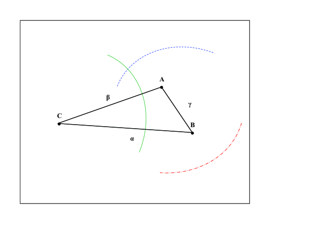
Figure 1: A configuration of the three atoms A, B, C at time $t$ such that $\alpha>ct$, $\beta>ct$ and $\gamma<ct$, for which a nonlocal behaviour of the interaction energy $\Delta E_{C}(A,B)$ is found. Red, blue and green (long-dash-dot, dashed and continuous lines, respectively) circumference’s arcs of radius $ct$ represent respectively the causality spheres of atoms A, B and C at time $t$.

IV The time-dependent three-body CP potential between atoms A,B and C

We now evaluate the following quantity, obtained by a symmetrization of the interaction energies of any pairs of atoms in the presence of the third one

$$\Delta E(A,B,C)$$ (24)

$$=\frac{2}{3}\Biggl{(}\sum_{{\bf k}j{{\bf k}^{\prime}}j^{\prime}}\alpha_{A}(k)\alpha_{B}(k^{\prime})$$

$$\times\langle E_{\ell}({\bf k}j,{\bf r}_{A},t)E_{m}({{\bf k}^{\prime}}j^{\prime},{\bf r}_{B},t)\rangle_{nr}V_{\ell m}(k,k^{\prime},\gamma)$$

$$+(A\rightarrow B\rightarrow C)\Biggr{)}$$

$$+\sum_{{\bf k}j{{\bf k}^{\prime}}j^{\prime}}\alpha_{A}(k)\alpha_{B}(k^{\prime})\langle E_{\ell}({\bf k}j,{\bf r}_{A},t)E_{m}({{\bf k}^{\prime}}j^{\prime},{\bf r}_{B},t)\rangle_{r}$$

$$\times V_{\ell m}^{r}(k_{0},\gamma)$$

where $(A\rightarrow B\rightarrow C)$ indicates terms obtained from the first double sum by a permutation of the atomic indices. In stationary cases this quantity has been shown to be equivalent to the three-body Casimir-Polder potential, as obtained by sixth-order perturbation theory PPR05 . This motivates our choice to consider this physical quantity. We stress that we symmetrize only on the nonresonant part, for which the role of the three atoms is indeed symmetrical; the resonant part should not be symmetrized because the contribution of the three atoms to this term is not symmetrical, only C being in an excited state.

We now wish to investigate if the nonlocal aspect discussed above for the interaction energy $\Delta E_{C}(A,B)$ are present in $\Delta E(A,B,C)$ too. Explicit evaluation of (24), yields

$$\Delta E(A,B,C)=\Delta E_{(I)}(A,B,C)+\Delta E_{(II)}(A,B,C)$$ (25)

$$+\Delta E_{(r)}(A,B,C)$$

where

$$\Delta E_{(I)}(A,B,C)=\frac{\hbar c}{12\pi}F_{\ell n}^{\alpha}F_{mp}^{\beta}F_{\ell m}^{\gamma}\frac{1}{\alpha\beta\gamma}\,\Biggl{\{}\,\int_{0}^{\infty}\,\,du\alpha_{A}(iu)\alpha_{B}(iu)\alpha_{C}(iu)\biggl{[}e^{-u(\alpha+\beta+\gamma)}\biggl{(}6$$ (26)

$$-\,\,\mbox{sgn}(\alpha-ct)-\mbox{sgn}(\beta-ct)-\mbox{sgn}(\gamma-ct)-\mbox{sgn}(\alpha+\beta-ct)-\mbox{sgn}(\alpha+\gamma-ct)$$

$$-\mbox{sgn}(\gamma+\beta-ct)\biggr{)}$$

$$+\,\,e^{-u(\alpha-\beta+\gamma)}\biggl{(}-\mbox{sgn}(\beta-ct)+\mbox{sgn}(\alpha+\gamma-ct)\biggr{)}+e^{-u(\alpha+\beta-\gamma)}\biggl{(}-\mbox{sgn}(\gamma-ct)$$

$$+\mbox{sgn}(\alpha+\beta-ct)\biggr{)}$$

$$+\,\,e^{-u(-\alpha+\beta+\gamma)}\biggl{(}-\mbox{sgn}(\alpha-ct)+\mbox{sgn}(\beta+\gamma-ct)\biggr{)}\biggr{]}\Biggr{\}};$$

and

$$\Delta E_{(II)}(A,B,C)=\frac{\hbar c}{12\pi}F_{\ell n}^{\beta}F_{mp}^{\alpha}F_{\ell m}^{\gamma}\frac{1}{\alpha\beta\gamma}\,\Biggl{\{}2\alpha_{B}(k_{0})\biggl{[}\cos k_{0}(\alpha-ct)\int_{0}^{\infty}\,du\,\alpha_{A}(iu)\alpha_{C}(iu)$$ (27)

$$\times\biggl{(}e^{-u(\beta+\gamma+ct)}+\mbox{sgn}(\beta+\gamma-ct)e^{-u|\beta+\gamma-ct|}+\mbox{sgn}(\beta-\gamma-ct)e^{-u|\beta-\gamma-ct|}$$

$$+\mbox{sgn}(\beta-\gamma+ct)e^{-u|\beta-\gamma+ct|}\biggr{)}$$

$$+\,\,\frac{\sin k_{0}(\alpha-ct)}{k_{0}}\int_{0}^{\infty}\,du\,\,u\,\alpha_{A}(iu)\alpha_{C}(iu)\biggl{(}e^{-u(\beta+\gamma+ct)}+e^{-u|\beta+\gamma-ct|}+e^{-u|\beta-\gamma-ct|}-e^{-u|\beta-\gamma+ct|}\biggr{)}$$

$$+\,(B\rightleftharpoons C,\,\beta\rightleftharpoons\gamma)\biggr{]}\theta(ct-\alpha)+4\alpha_{A}(k_{0})\biggl{[}\cos k_{0}(\beta+\gamma-ct)\int_{0}^{\infty}du\,\alpha_{B}(iu)\alpha_{C}(iu)\Big{(}e^{-u(\alpha+ct)}$$

$$+\,\,\mbox{sgn}(\alpha-ct)e^{-u|\alpha-ct|}\Big{)}+\frac{\sin k_{0}(\beta+\gamma-ct)}{k_{0}}\int_{0}^{\infty}du\,u\,\alpha_{B}(iu)\alpha_{C}(iu)\Big{(}e^{-u(\alpha+ct)}+e^{-u|\alpha-ct|}\Big{)}\biggr{]}$$

$$\times\theta(ct-(\beta+\gamma))$$

$$+\,\,(A\rightleftharpoons B,\,\,\alpha\rightleftharpoons\beta)+(A\rightleftharpoons C,\,\,\alpha\rightleftharpoons\gamma)\Biggr{\}};$$

are the nonresonant contributions, while

$$\Delta E(A,B,C)_{(r)}=-\mu_{n}^{12}\mu_{p}^{12}\alpha_{A}(k_{0})\alpha_{B}(k_{0})2\Re(F_{\ell n}^{\beta}F_{mp}^{\alpha}\frac{e^{ik_{0}(\beta-\alpha)}}{\alpha\beta})F_{\ell m}^{\gamma}(\frac{\cos k_{0}\gamma}{\gamma})\theta(ct-\beta)\theta(ct-\alpha)$$ (28)

is the resonant one. We have assumed isotropic atoms, that is $\mbox{\boldmath$\mu$}_{i}\mbox{\boldmath$\mu$}_{j}=\frac{1}{3}|\mbox{\boldmath$\mu$}|^{2}$, and $\alpha(iu)$ is the dynamic polarizability extended to imaginary frequencies.

Eq. (25) describes the time-dependent symmetrized three-body CP potential as a function of time for a generic configuration of the three atoms (for times shorter than the spontaneous decay time of the excited atom, due to the limitations of our perturbative treatment). As in the case discussed in the previous Section, we now consider specific cases relevant for our discussion about nonlocal aspects of the dynamical interaction energy. First of all, it is immediate to see that $\Delta E(A,B,C)$ vanishes if each atom is outside the light cone of the other two, that is for $\alpha,\beta,\gamma>ct$. On the contrary, $\Delta E(A,B,C)$ is non-vanishing for times such that each atom is separated by a time-like interval from the other two. In particular, for large times, the time-dependent terms rapidly decrease to zero and we find the well-known stationary result PPR05 . This means that after a transient characterized by a time-dependent interaction, the three-body interaction energy settles to the time-independent Casimir-Polder interaction between three atoms with an excited atoms. All these results are compatible with relativistic causality and similar to those previously obtained for the dynamical three-body Casimir-Polder interaction between three ground-state atoms PPR06 . However, when the spatial configuration of the three atoms is such that two of them are separated by a time-like distance we find a non-vanishing three-body interaction, even if the third atom is outside their causality sphere. For example, when the separation of A from the other two atoms is space-like, Eq.(25) yields

$$\Delta E(A,B,C)=\frac{\hbar c}{6\pi}F_{mp}^{\alpha}F_{\ell n}^{\beta}F_{\ell m}^{\gamma}\frac{1}{\alpha\beta\gamma}\int_{0}^{\infty}\!du\!\alpha_{A}(iu)\alpha_{B}(iu)\alpha_{C}(iu)(e^{-u(\alpha+\beta+\gamma)}+e^{-u(-\alpha+\beta+\gamma)})$$ (29)

$$-\frac{1}{6\pi}\mu^{12}_{n}\mu^{12}_{p}F_{mp}^{\alpha}F_{\ell n}^{\beta}F_{\ell m}^{\gamma}\frac{1}{\alpha\beta\gamma}2\Re\Biggl{\{}\,\alpha_{B}(k_{0})e^{-ik_{0}(\alpha-ct)}\int_{0}^{\infty}\,dk\,\alpha_{A}(k)\frac{\sin k(\beta+\gamma)}{k_{0}+k}e^{i\omega_{k}t}\Biggr{\}}$$

$$-\frac{1}{6\pi}\mu_{n}^{12}\mu_{p}^{12}F_{mp}^{\alpha}F_{\ell n}^{\beta}F_{\ell m}^{\gamma}\frac{1}{\alpha\beta\gamma}2\Re\Biggl{\{}\,\alpha_{C}(k_{0})e^{-ik_{0}(\alpha-ct)}\int_{0}^{\infty}\,dk\,\alpha_{A}(k)\frac{\sin k(\beta+\gamma)}{k_{0}+k}e^{i\omega_{k}t}\Biggr{\}}$$

which in general does not vanish. Thus the nonlocal features of field emitted by the atoms during their self-dressing are evident also in the three-body interaction energy $\Delta E(A,B,C)$, with features which may differ from to those of $\Delta E_{C}(A,B)$. Eq.(29) shows also that the nonlocal features of $\Delta E(A,B,C)$ stem from the non-resonant contributions, so that they are exclusively due to the virtual photons dressing the atoms, as we have recently discussed in the case of ground-state atoms PPR06 .

V Conclusions

We have considered the Casimir-Polder interaction energy between three atoms with one atom initially in its excited state, using a time-dependent approach. We have discussed the problem of relativistic causality in the interaction between the atoms and its connection with the non-locality of spatial field correlations. The spatial correlation function of the field emitted during the spontaneous decay of the excited atom has been first obtained. We have shown that a non-local behaviour appears, in agreement with previous results, and that it is related to a non-resonant contribution related to the emission of virtual photons. We have shown that a non-local behaviour appears also in the dynamical Casimir-Polder interaction between two other ground-state atoms, during the initial stage of the spontaneous decay of the first atom. We have suggested that the appearance of this non-local behaviour can be ascribed to the non-locality of the field correlation function and that this new phenomenon should be observable. Thus we conclude that the nonlocal properties of the electromagnetic field emitted by the atoms during their dynamical self-dressing may become manifest in the time-dependence of the Casimir-Polder potential. We remark that previous studies of causality in the time-dependent two-body Casimir-Polder interaction have not shown indications of non local behaviour RPP04 . Hence the causality problem appears quite more complicated and subtle in the case of the time-dependent three-body Casimir-Polder energy, where nonlocal aspects may become manifest.

References

• (1) H.B.G. Casimir, Proc. K. Ned. Akad. Wet. B 51 (1948) 793
• (2) H.B.G. Casimir, D. Polder, Phys. Rev. 73 (1948) 360
• (3) C.I. Sukenik, M.G. Boshier, D. Cho, V. Sandoghdar, E.A. Hinds, Phys.Β Rev.Β Lett.Β 70 (1993) 560.
• (4) S.K. Lamoreaux, Phys. Rev. Lett. 78, 5 (1997)
• (5) M. Bordag, U. Mohideen, V.M. Mostepanenko, Phys.Β Rep.Β 353, 1 (2001).
• (6) D. Iannuzzi, M. Lisanti, F. Capasso, Proc. Nat. Ac. Sci. 101, 4019 (2004)
• (7) S.A. Fulling and P.C.W. Davies, Proc.Β R.Β Soc.Β LondonΒ A 348, 393 (1976).
• (8) M. Kardar and R. Golestanian, Rev.Β Mod.Β Phys.Β 71, 1233 (1999).
• (9) W.G. Unruh, Phys.Β Rev.Β DΒ 14, 870 (1976).
• (10) E.A. Power, T. Thirunamachandran, Phys.Β Rev.Β AΒ 48 (1993) 4761.
• (11) R. Passante, F. Persico, L. Rizzuto, Phys. Lett. A 316, 29 (2003)
• (12) M. Cirone, R. Passante, J. Phys. B: At. Mol. Opt. Phys. 40, 5579 (1997)
• (13) R. Passante, F. Persico, and L. Rizzuto, J. Mod. Opt. 52, 1957 (2005)
• (14) C.G. Hegerfeldt, Phys. Rev. Lett. 72, 596 (1994)
• (15) G. Compagno, G. M. Palma, R. Passante, and F. Persico, in The Physics of Communication: Proceeding of the XXII nd Solvay Conference in Physics, I. Antoniou, V.A. Sadovnichy, H. Walter eds., World Scientific, Singapore, 2003, p. 389
• (16) P. W. Milonni, D. F. V. James, and H. Fearn, Phys. Rev. A. 52, 1525 (1995)
• (17) E. A. Power, T. Thirunamachandran, Phys. Rev. A 56, 3395 (1997)
• (18) T. Petrosky, G. Ordonez, I. Prigogine, Phys. Rev. A 62, 42106 (2000)
• (19) T. Petrosky, G. Ordonez, I. Prigogine, Phys. Rev. A 64, 62101 (2001)
• (20) I. Antoniou, E. Karpov, G. Pronko, Found. of Phys. 31, 1641 (2001)
• (21) A. K. Biswas, G. Compagno, G. M. Palma, R. Passante, and F. Persico, Phys. Rev. A. 42, 4291 (1990)
• (22) A. La Barbera, R. Passante, Phys. Lett. A 206, 1 (1995)
• (23) W. G. Unruh, R. M. Wald, Phys.Β Rev.Β DΒ 29, 1047 (1984).
• (24) L. Rizzuto, R. Passante, F. Persico, Phys. Rev. A 70, 012107 (2004)
• (25) R. Passante, F. Persico, and L. Rizzuto, J. Phys. B. 39, S685 (2006)
• (26) D. P. Craig and T. Thirunamachandran, Molecular Quantum electrodynamics, Academic Press (1984)
• (27) E.A. Power, S. Zienau, Phil. Trans. Roy. Soc. London A 251, 427 (1959)
• (28) E. A. Power, T. Thirunamachandran, Phys. Rev. A 28, 2663 (1983)
• (29) E. A. Power, T. Thirunamachandran, Phys. Rev. A 60, 4927 (1999)