Non-Markovian Decay and Lasing Condition in an Optical Microcavity Coupled to a Structured Reservoir

Abstract

The decay dynamics of the classical electromagnetic field in a leaky optical resonator supporting a single mode coupled to a structured continuum of modes (reservoir) is theoretically investigated, and the issue of threshold condition for lasing in presence of an inverted medium is comprehensively addressed. Specific analytical results are given for a single-mode microcavity resonantly coupled to a coupled resonator optical waveguide (CROW), which supports a band of continuous modes acting as decay channels. For weak coupling, the usual exponential Weisskopf-Wigner (Markovian) decay of the field in the bare resonator is found, and the threshold for lasing increases linearly with the coupling strength. As the coupling between the microcavity and the structured reservoir increases, the field decay in the passive cavity shows non exponential features, and correspondingly the threshold for lasing ceases to increase, reaching a maximum and then starting to decrease as the coupling strength is further increased. A singular behavior for the ”laser phase transition”, which is a clear signature of strong non-Markovian dynamics, is found at critical values of the coupling between the microcavity and the reservoir.

I Introduction.

It is well known that the modes of an open optical cavity are always leaky due to energy escape to the outside. Mode leakage can be generally viewed as due to the coupling of the discrete cavity modes with a broad spectrum of modes of the ”universe” that acts as a reservoir Lang73 ; Ching87 ; Ching98 . From this perspective the problem of escape of a classical electromagnetic field from an open resonator is analogous to the rather general problem of the decay of a discrete state coupled to a broad continuum, as originally studied by Fano Fano64 and encountered in different physical contexts (see, e.g., Tannoudji ). The simplest and much used way to account for mode coupling with the outside is to eliminate the reservoir degrees of freedom by the introduction of quasi normal modes with complex eigenfrequencies (see, e.g., Lang73 ; Ching98 ), in such a way that energy escape to the outside is simply accounted for by the cavity decay rate $\gamma$ (the imaginary part of the eigenvalue) or, equivalently, by the cavity quality factor $Q$. This irreversible exponential decay of the mode into the continuum corresponds to the well-known Weisskopf-Wigner decay and relies on the so-called Markovian approximation (see, e.g., Tannoudji ) that assumes an instantaneous reservoir response (i.e. no memory): coupling with the reservoir is dealt as a Markovian process and the evolution of the field in the cavity depends solely on the present state and not on any previous state of the reservoir. For the whole system (cavity plus outside), in the Markovian approximation the cavity quasi-mode with a complex frequency corresponds to a resonance state with a Lorentzian lineshape. If now the field in the cavity experiences gain due to coupling with an inverted atomic medium, the condition for lasing is simply obtained when gain due to lasing atoms cancels cavity losses, i.e. for $g=\gamma$, where $g$ is the modal gain coefficient per unit time Lang73 . More generally, treating the field classically and assuming that the cavity supports a single mode, an initial field amplitude in the cavity will exponentially decay, remain stationary (delta-function lineshape) or exponentially grow (in the early stage of lasing) depending on whether $g<\gamma$, $g=\gamma$ or $g>\gamma$, respectively. In addition, since the cavity decay rate $\gamma$ increases as the coupling of the cavity with the outside increases, the threshold for laser oscillation increases as the coupling strength of the resonator with the modes of the ”universe” is increased. It is remarkable that this simple and widely acknowledged dynamical behavior of basic laser theory, found in any elementary laser textbook (see, e.g., Svelto ), relies on the Markovian assumption for the cold cavity decay dynamics note0 . However, it is known that in many problems dealing with the decay of a discrete state coupled to a ”structured” reservoir, such as in photoionization in the vicinity of an autoionizing resonance Piraux90 , spontaneous emission and laser-driven atom dynamics in waveguides and photonic crystals Lai88 ; Lewenstein88 ; John90 ; John94 ; Kofman94 ; Vats98 ; Lambropoulos00 ; Wang03 ; Petrosky05 , and electron transport in semiconductor superlattices Tanaka06 , the Markovian approximation may become invalid, and the precise structure of the reservoir (continuum) should be properly considered. Non-Markovian effects may become of major relevance in presence of threshold Piraux90 ; Gaveau95 or singularities Lewenstein88 ; John94 ; Kofman94 ; Lambropoulos00 ; Tanaka06 in the density of states or more generally when the coupling strength from the initial discrete state to the continuum becomes as large as the width of the continuum density of state distribution Tannoudji . Typical features of non-Markovian dynamics found in the above-mentioned contexts are non-exponential decay, fractional decay and population trapping, atom-photon bound states, damped Rabi oscillations, etc. Though the role of structured reservoirs on basic quantum electrodynamics and quantum optics phenomena beyond the Markovian approximation has received a great attention (see, e.g., Ref.Lambropoulos00 for a rather recent review), at a classical level Ching98 previous works have mainly considered the limit of Markovian dynamics Lang73 , developing a formalism based on quasi-normal mode analysis of the open system Ching98 . In fact, in a typical laser resonator made e.g. of two-mirrors with one partially transmitting mirror coupled to the outside open space, the Weisskopf-Wigner decay law for the bare cavity field is an excellent approximation Lang73 and therefore non-Markovian effects are fully negligible. However, the advent of micro- and nano-photonic structures, notably photonic crystals (PCs), has enabled the design and realization of high-$Q$ passive microcavities Villeneuve96 ; Vahala03 ; Armani03 ; Asano04 ; Asano06 and lasers Vahala03 ; Painter99 ; Loncar02 ; Park04 ; Altug05 which can be suitably coupled to the outside by means of engineered waveguide structures Vahala03 ; Fan98 ; Xu00 ; Asano03 ; Waks05 ; Chak06 . By e.g. modifying some units cells within a PC, one can create defects that support localized high-$Q$ modes or propagating waveguide modes. If we couple localized defect modes with waveguides, many interesting photon transport effects may occur (see, e.g., Fan98 ; Xu00 ; Fan05 ). Coupling between optical waveguides and high-$Q$ resonators in different geometries has been investigated in great detail using numerical methods, coupled-mode equations, and scattering matrix techniques in the framework of a rather general Fano-Anderson-like Hamiltonian Fan98 ; Xu00 ; Asano03 ; Waks05 ; LanLan05 ; Chak06 . Another kind of light coupling and transport that has received an increasing attention in recent years is based on coupled resonator optical waveguide (CROW) structures Stefanou98 ; Yariv99 ; Ozbay00 ; Olivier01 , in which photons hop from one evanescent defect mode of a cavity to the neighboring one due to overlapping between the tightly confined modes at each defect site. The possibility of artificially control the coupling of a microcavity with the ”universe” may then invalidate the usual Markovian approximation for the (classical) electromagnetic field decay. In such a situation, for the passive cavity one should expect to observe non-Markovian features in the dynamics of the decaying field, such as non-exponential decay, damped Rabi oscillations, and quenched decay for strong couplings. More interesting, for an active (i.e. with gain) microcavity the usual condition $g=\gamma$ of gain/loss balance for laser oscillation becomes meaningless owing to the impossibility of precisely define a cavity decay rate $\gamma$. Therefore the determination of the lasing condition for a microcavity coupled to a structured reservoir requires a detailed account of the mode structure of the universe and may show unusual features.
It is the aim of this work to provide some general insights into the classical-field decay dynamics and lasing condition of an optical microcavity coupled to a structured reservoir, in which the usual Markovian approximation of treating the cavity decay becomes inadequate. Some general results are provided for a generic Hamiltonian model describing the coupling of a single-mode microcavity with a continuous band of modes, and the effects of non-Markovian dynamics on lasing condition are discussed. As an illustrative example, the case of a microcavity resonantly coupled to a CROW is considered, for which analytical results may be given in a closed form.
The paper is organized as follows. In Sec.II a simple model describing the classical field dynamics in an active single-mode microcavity coupled to a band of continuous modes is presented, and the Markovian dynamics attained in the weak coupling regime is briefly reviewed. Section III deals with the exact dynamics, beyond the Markovian approximation, for both the passive (i.e. without gain) and active microcavity. In particular, the general relation expressing threshold for laser oscillation is derived, and its dependence on the coupling strength between the microcavity and the reservoir is discussed. The general results of Sec.III are specialized in Sec.IV for the case of a single-mode microcavity tunneling-coupled to a CROW, and some unusual dynamical effects (such as ”uncertainty” of laser threshold, non-exponential onset of lasing instability and transient non-normal amplification) are shown to occur at certain critical couplings.

II Microcavity coupled to a structured reservoir: description of the model and Markovian dynamics

II.1 The model

The starting point of our analysis is provided by a rather general Hamiltonian model Fan98 ; Xu00 describing the interaction of a localized mode $|a\rangle$ of a resonator system (e.g. a microcavity in a PC) with a set of continuous modes $|\omega_{\mu}\rangle$ of neighboring waveguides with which the resonator is tunneling-coupled. We assume that the microcavity supports a single and high-$Q$ localized mode of frequency $\omega_{a}$, and indicate by $\gamma_{i}$ and $g$ the intrinsic losses and gain coefficients of the mode. The intrinsic losses $\gamma_{i}$ account for both internal (e.g. absorption) losses and damping of the cavity mode due to coupling with a ”Markovian” reservoir (i.e. coupling with modes of the universe other than the neighboring waveguides). The modal gain parameter $g$ may be provided by an inverted atomic or semiconductor medium hosted in the microcavity. Since we will consider the microcavity operating below or at the onset of threshold for lasing, as in Refs.Xu00 ; LanLan05 the modal gain parameter $g$ is assumed to be a constant and externally controllable parameter; above threshold an additional rate equation for $g$ would be obviously needed depending on the specific gain medium (see, for instance, Liu05 ). Dissipation and gain of the microcavity mode are simply included in the model by adding a non-Hermitian term $H_{NH}$ to the Hermitian part of the Hamiltonian. The full Hamiltonian $H$ then reads $H=H_{0}+H_{int}+H_{NH}$, where Fan98

$$H_{0} = \omega_{a}|a\rangle\langle a|+\sum_{\mu}\int d\omega_{\mu}\omega_{\mu}|\omega_{\mu}\rangle\langle\omega_{\mu}|,$$ (1a)

$$H_{int} = \lambda\sum_{\mu}\int d\omega_{\mu}\left[\kappa_{\mu}(\omega_{\mu})|\omega_{\mu}\rangle\langle a|+h.c.\right],$$ (1b)

$$H_{NH} = i(g-\gamma_{i})|a\rangle\langle a|,$$ (1c)

with $\langle a|a\rangle=1$, $\langle\omega_{\mu}|\omega^{{}^{\prime}}_{\mu^{{}^{\prime}}}\rangle=\delta_{\mu,\mu^{{}^{\prime}}}\delta(\omega_{\mu}-\omega^{{}^{\prime}}_{\mu})$, $\langle a|\omega_{\mu}\rangle=0$, and $\hbar=1$. The coefficients $\kappa_{\mu}(\omega_{\mu})$ describe the direct coupling between the localized mode $|a\rangle$ of the microcavity and the propagating modes $|\omega_{\mu}\rangle$ in the continuum, whereas $\lambda$ is a dimensionless parameter that measures the strength of interaction ($\lambda\rightarrow 0$ for a vanishing interaction). If we write the state $|\psi\rangle$ as

$$|\psi\rangle=c_{a}(t)|a\rangle+\sum_{\mu}\int d\omega_{\mu}c_{\mu}(\omega_{\mu},t)|\omega_{\mu}\rangle$$ (2)

the following coupled-mode equations for the coefficients $c_{a}(t)$ and $c_{\mu}(\omega_{\mu},t)$ are readily obtained from the equation $i\partial|\psi\rangle/\partial t=H|\psi\rangle$:

$$i\dot{c}_{a}(t) = (\omega_{a}+ig-i\gamma_{i})c_{a}(t)+\lambda\sum_{\mu}\int d\omega_{\mu}\kappa_{\mu}^{*}(\omega_{\mu})c_{\mu}(\omega_{\mu},t),$$ (3a)

$$i\dot{c}_{\mu}(\omega_{\mu},t) = \omega_{\mu}c_{\mu}(\omega_{\mu},t)+\lambda\kappa_{\mu}(\omega_{\mu})c_{a}(t),$$ (3b)

where the dot stands for the derivative with respect to time $t$. Note that the power of the microcavity mode is given by $|c_{a}(t)|^{2}$, whereas the total power of the field (cavity plus structured reservoir) is given by $P(t)=|c_{a}(t)|^{2}+\sum_{\mu}\int d\omega_{\mu}|c_{\mu}(\omega_{\mu},t)|^{2}$. The threshold condition for lasing is obtained when an initial perturbation in the system does not decay with time. From Eqs.(3a) and (3b) the following power-balance equation can be derived

$$\frac{dP}{dt}=(g-\gamma_{i})|c_{a}|^{2},$$ (4)

from which we see that $|c_{a}|^{2}\rightarrow 0$ for any $g<\gamma_{i}$, so that the threshold $g=g_{th}$ for laser oscillation satisfies the condition $g_{th}\geq\gamma_{i}$, as expected.

II.2 Weak coupling limit: Markovian dynamics

The temporal evolution of the microcavity-mode amplitude $c_{a}(t)$ and the condition for laser oscillation can be rigorously obtained by solving the coupled-mode equations (3a) and (3b) by means of a Laplace transform analysis, which will be done in the next section. Here we show that, in the weak coupling regime ($\lambda\rightarrow 0$) and for a broad band of continuous modes, coupling of the cavity mode with the neighboring waveguides leads to the usual Weisskopf-Wigner (exponential) decay. Though this is a rather standard result (see, e.g. Tannoudji ) and earlier derived for a standard Fabry-Perot laser resonator in Ref.Lang73 using a Fano diagonalization technique, for the sake of completeness it is briefly reviewed here within the model described in Sec.II.A. If the system is initially prepared in state $|a\rangle$, i.e. if at initial time $t=0$ there is no field in the neighboring waveguides and $c_{a}(0)\neq 0$, an integro-differential equation describing the temporal evolution of cavity mode amplitude $c_{a}(t)$ at successive times can be derived after elimination of the reservoir degrees of freedom. A formal integration of Eqs.(3b) with initial condition $c_{\mu}(\omega_{\mu},0)=0$ yields

$$c_{\mu}(\omega_{\mu},t)=-i\lambda\kappa_{\mu}(\omega_{\mu})\int_{0}^{t}dt^{\prime}c_{a}(t^{\prime})\exp[-i\omega_{\mu}(t-t^{\prime})].$$ (5)

After setting $c_{a}(t)=A(t)\exp(-i\omega_{a}t)$, substitution of Eq.(5) into Eq.(3a) yields the following exact integro-differential equation for the mode amplitude $A(t)$

$$\dot{A}=(g-\gamma_{i})A-\int_{0}^{t}d\tau G(\tau)A(t-\tau),$$ (6)

where $G(\tau)$ is the reservoir response (memory) function, given by

$$G(\tau)=\lambda^{2}\sum_{\mu}\int d\omega_{\mu}|\kappa_{\mu}(\omega_{\mu})|^{2}\exp[-i(\omega_{\mu}-\omega_{a})\tau].$$ (7)

Equation (6) clearly shows that the dynamics is not a Markovian process since the evolution of the mode amplitude at time $t$ depends on previous states of the reservoir. Nevertheless, if the characteristic memory time $\tau_{m}$ is short enough (i.e., the spectral coupling coefficients $\kappa_{\mu}$ broad enough) and the coupling weak enough such that $|\dot{A}/A|\tau_{m}\ll 1$, we may replace Eq.(6) with the following approximate equation

$$\dot{A}\simeq(g-\gamma_{i})A-A(t)\int_{0}^{t}d\tau G(\tau)\simeq(g-\gamma_{i})A-(\gamma_{R}+i\Delta_{R})A,$$ (8)

where

$$(\gamma_{R}+i\Delta_{R})=\int_{0}^{t}d\tau G(\tau)$$ (9)

for $t\gg\tau_{m}$. In this limit, the dynamics is therefore Markovian and the reservoir is simply accounted for by a decay rate $\gamma_{R}$ and a frequency shift $\Delta_{R}$. Using the relation

$$\lim_{t\rightarrow\infty}\int_{0}^{t}d\tau\exp(-i\omega\tau)=\pi\delta(\omega)-i\mathcal{P}\left(\frac{1}{\omega}\right),$$ (10)

from Eq.(7) the following expressions for the decay rate $\gamma_{R}$ and the frequency shift $\Delta_{R}$ can be derived

$$\gamma_{R} = \pi\lambda^{2}\sum_{\mu}|\kappa_{\mu}(\omega_{a})|^{2},$$ (11)

$$\Delta_{R} = \lambda^{2}\sum_{\mu}\mathcal{P}\int d\omega_{\mu}\frac{|\kappa_{\mu}(\omega_{\mu})|^{2}}{\omega_{a}-\omega_{\mu}}.$$ (12)

The dynamics of the cavity mode field in the Markovian approximation is therefore standard: an initial field amplitude in the cavity will exponentially decay, remain stationary (delta-function lineshape) or exponentially grow (in the early stage of lasing) depending on whether $g<\gamma$, $g=\gamma$ or $g>\gamma$, respectively, where $\gamma=\gamma_{i}+\gamma_{R}$ is the total cavity decay rate. The threshold for laser oscillation is therefore simply given by $g_{th}=\gamma_{i}+\gamma_{R}$, i.e.

$$g_{th}=\gamma_{i}+\pi\lambda^{2}\sum_{\mu}|\kappa_{\mu}(\omega_{a})|^{2}.$$ (13)

III Field Dynamics beyond the Markovian Limit: general aspects

Let us assume that the system is initially prepared in state $|a\rangle$, i.e. that at initial time $t=0$ there is no field in the neighboring waveguides [$c_{\mu}(\omega_{\mu},0)=0$] whereas $c_{a}(0)=1$. The exact solution for the field amplitude $c_{a}(t)$ of the microcavity mode at successive times can be obtained by a Laplace-Fourier transform of Eqs.(3a) and (3b). Let us indicate by $\hat{c_{a}}(s)$ and $\hat{c_{\mu}}(\omega_{\mu},s)$ the Laplace transforms of $c_{a}(t)$ and ${c_{\mu}}(\omega_{\mu},t)$, respectively, i.e.

$$\hat{c_{a}}(s)=\int_{0}^{\infty}dt\;c_{a}(t)\exp(-st)$$ (14)

and a similar expression for $\hat{c_{\mu}}(\omega_{\mu},s)$. From the power balance equation (4), one can easily show that the integral on the right hand side in Eq.(14) converges for ${\rm Re}(s)>\eta$, where $\eta=0$ for $g-\gamma_{i}\leq 0$ or $\eta=g-\gamma_{i}$ for $g-\gamma_{i}>0$. The field amplitude $c_{a}(t)$ is then written as the inverse Laplace transform

$$c_{a}(t)=\frac{1}{2\pi i}\int_{{\rm B}}ds\;\hat{c}_{a}(s)\exp(st)$$ (15)

where the Bromwich path ${\rm B}$ is a vertical line ${\rm Re}(s)={\rm const}>\eta$ in the half-plane of analyticity of the transform, and $\hat{c}_{a}(s)$ is readily derived after Laplace transform of Eqs.(3a) and (3b) and reads

$$\hat{c}_{a}(s)=\frac{i}{is-\omega_{a}-ig^{\prime}-\Sigma(s)}$$ (16)

In Eq.(16), $g^{\prime}=g-\gamma_{i}$ is the effective gain parameter and $\Sigma(s)$ is the self-energy function, which is expressed in terms of the form factor

$$\Sigma(s)=\int_{\omega_{1}}^{\omega_{2}}d\omega\frac{\mathcal{D}(\omega)}{is-\omega}$$ (17)

where $\mathcal{D}(\omega)$ is the reservoir structure function, defined by

$$\mathcal{D}(\omega)=\lambda^{2}\sum_{\mu}|\kappa_{\mu}(\omega)|^{2}.$$ (18)

In writing Eq.(17), we assumed that the spectrum of modes of the waveguides (to which the microcavity is coupled) shows an upper and lower frequency limits $\omega_{1}$ and $\omega_{2}$. We will also assume that $\mathcal{D}(\omega)$ does not show gaps, i.e. intervals with $\mathcal{D}=0$, inside the range $(\omega_{1},\omega_{2})$. The assumption of a finite spectral extension for the continuous modes is physically reasonable and is valid for e.g. PC waveguides or CROW. In addition, in order to avoid the existence of bound states (or polariton modes) for the passive microcavity coupled to the structured reservoir, we assume that $\mathcal{D}(\omega)$ vanishes at the boundary of the band, precisely we require that $\mathcal{D}(\omega)\sim(\omega-\omega_{1,2})^{\delta_{1,2}}$ as $\omega\rightarrow\omega_{1,2}$, with $\delta_{1,2}>0$. This condition, which will be clarified in Sec.III.A, is a necessary requirement to ensure that the field amplitude $c_{a}(t)$ fully decays toward zero for $g^{\prime}=0$.
The temporal evolution of $c_{a}(t)$ is largely influenced by the analytic properties of $\hat{c}_{a}(s)$; in particular the occurrence of a singularity (pole) at $s=s_{pole}$ with ${\rm Re}(s_{pole})\geq 0$ may indicate the onset of an instability, i.e. a lasing regime. The self-energy function $\Sigma(s)$ [Eq.(17)], and hence $\hat{c}_{a}(s)$, are not defined on the segment of the imaginary axis $s=-i\omega$ with $\omega_{1}<\omega<\omega_{2}$, $s_{1,2}=-i\omega_{1,2}$ being two branch points. In fact, using the relation

$$\lim_{\rho\rightarrow 0^{+}}\frac{1}{\omega\pm i\rho}=\mathcal{P}\left(\frac{1}{\omega}\right)\mp i\pi\delta(\omega),$$ (19)

from Eq.(17) one has

$$\Sigma(s=-i\omega\pm 0^{+})=\Delta(\omega)\mp i\pi\mathcal{D}(\omega),$$ (20)

($\omega_{1}<\omega<\omega_{2}$), where we have set

$$\Delta(\omega)=\mathcal{P}\int_{\omega_{1}}^{\omega_{2}}d\omega^{\prime}\frac{\mathcal{D}(\omega^{\prime})}{\omega-\omega^{\prime}}.$$ (21)

To further discuss the analytic properties of $\hat{c}_{a}(s)$ and hence the temporal dynamics of $c_{a}(t)$, one should distinguish the cases of passive ($g^{\prime}=0$) and active ($g^{\prime}>0$) microcavities.

III.1 The passive microcavity

Let us first consider the case of $g^{\prime}=0$, i.e. of a passive microcavity with negligible internal losses. In this case the full Hamiltonian is Hermitian ($H_{NH}=0$), and therefore the analytic properties of $\hat{c}_{a}(s)$ and spectrum of $H=H_{0}+H_{int}$ are ruled as follows (see, for instance, Tannoudji ; Gaveau95 ; Nakazato96 ; Regola ): (i) The eigenvalues $\omega$ of $H$ are real-valued and comprise the continuous spectrum $\omega_{1}<\omega<\omega_{2}$ of unbounded modes and up to two isolated real-valued eigenvalues, outside the continuous spectrum from either sides, which correspond to possible bound (or polariton) modes Gaveau95 ; (ii) The isolated eigenvalues are the poles of $\hat{c}_{a}(s)$ on the imaginary axis outside the branch cut $-\omega_{2}<{\rm Im}(s)<-\omega_{1}$; (iii) $\hat{c}_{a}(s)$ is analytic in the full complex plane, apart from the branch cut and the two possible poles on the imaginary axis corresponding to bound modes; (iv) In the absence of bound modes $c_{a}(t)$ fully decays toward zero, whereas a limited (or fractional) decay occurs in the opposite case.
From Eq.(16), the poles $s=-i\Omega$ of $\hat{c}_{a}(s)$ outside the branch cut are found as solutions of the equation:

$$\Omega-\omega_{a}=\int_{\omega_{1}}^{\omega_{2}}d\omega\frac{\mathcal{D}(\omega)}{\Omega-\omega},$$ (22)

i.e. [see Eq.(21)]:

$$\Omega-\omega_{a}=\Delta(\Omega)$$ (23)

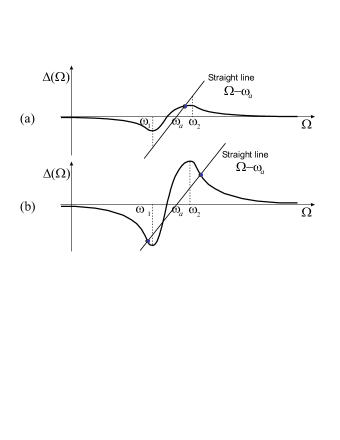
Figure 1: Graphical determination of the roots of Eq.(23) below (a), and above (b) the critical coupling. In (b) the full Hamiltonian $H=H_{0}+H_{int}$ has discrete eigenvalues corresponding to bound modes.

with the constraint $\Omega>\omega_{2}$ or $\Omega<\omega_{1}$ note1 . A graphical solution of Eq.(23) as intersection of the curves $\Omega-\omega_{a}$ and $\Delta(\Omega)$ is helpful to decide whether there exist poles of $\hat{c}_{a}(s)$, i.e. bound modes (see Fig.1). To this aim, note that $\Delta(\Omega)>0$ and $d\Delta/d\Omega<0$ for $\Omega>\omega_{2}$, $\Delta(\Omega)<0$ and $d\Delta/d\Omega<0$ for $\Omega<\omega_{1}$, and $\lim_{\Omega\rightarrow\pm\infty}\Delta(\Omega)=0^{\pm}$. Therefore, Eq.(23) does not have solutions outside the interval $(\omega_{1},\omega_{2})$ provided that $\Delta(\omega_{2})<\omega_{2}-\omega_{a}$ and $\Delta(\omega_{1})>\omega_{1}-\omega_{a}$ [Fig.1(a)]. Such conditions require at least that $\omega_{a}$ be internal to the band $(\omega_{1},\omega_{2})$, i.e. that the resonance frequency $\omega_{a}$ of the microcavity be embedded in the continuum of decay channels, and that $\mathcal{D}(\omega)$ vanishes as a power law at the boundary $\omega=\omega_{1}$ and $\omega=\omega_{2}$, i.e. that $\mathcal{D}(\omega)\sim(\omega-\omega_{1,2})^{\delta_{1,2}}$ as $\omega\rightarrow\omega_{1,2}$ for some positive integers $\delta_{1}$ and $\delta_{2}$. In fact, if $\mathcal{D}(\omega)$ does not vanish as a power law at these boundaries, one would have $\Delta(\Omega)\rightarrow\pm\infty$ as $\Omega\rightarrow\omega_{2},\omega_{1}$. Even though $\mathcal{D}(\omega)$ vanishes at the boundaries, as the coupling strength $\lambda$ is increased either one or both of the conditions $\Delta(\omega_{2})>\omega_{2}-\omega_{a}$ and $\Delta(\omega_{1})<\omega_{1}-\omega_{a}$ can be satisfied [Fig.1(b)], leading to the appearance of either one or two bound states. The coupling strength at which a bound state starts to appear is referred to as critical coupling. Below the critical coupling [Fig.1(a)], for the passive microcavity $\hat{c}_{a}(s)$ does not have poles and a complete decay of $c_{a}(t)$ is attained. However, owing to non-Markovian effects the decay dynamics may greatly deviate from the usual Weisskop-Wigner exponential decay. The exact decay law for $c_{a}(t)$ is obtained by the inverse Laplace transform Eq.(15), which can be evaluated by the residue method after suitably closing the Bromwich path ${\rm B}$ with a contour in the ${\rm Re}(s)<0$ half-plane (see, e.g. Tannoudji pp.220-221, and Nakazato96 ; Regola ). Since the closure crosses the branch cut $-\omega_{2}<{\rm Im}(s)<-\omega_{1}$ on the imaginary axis, the contour must necessarily pass into the second Riemannian sheet in the section of the half-plane with $-\omega_{2}<{\rm Im}(s)<-\omega_{1}$, whereas it remains in the first Riemannian sheet in the other two sections ${\rm Im}(s)>-\omega_{1}$ and ${\rm Im}(s)<-\omega_{2}$ of the ${\rm Re}(s)<0$ half-plane. To properly close the contour, it is thus necessary to go back and turn around the two branch points of the cut at $s=-i\omega_{1}$ and $s=-i\omega_{2}$, following the Hankel paths $h_{1}$ and $h_{2}$ as shown in Fig.2. Note that, while $\hat{c}_{a}(s)$ is analytic in the first Riemannian sheet for ${\rm Re}(s)<0$, the analytic continuation $\hat{c}_{a}^{II}(s)$ of $\hat{c}_{a}(s)$ from the right [${\rm Re}(s)>0$] to the left [${\rm Re}(s)<0$] half-plane across the cut has usually a simple pole at $s=s_{p}$ with ${\rm Re}(s_{p})<0$ and $-\omega_{2}<{\rm Im}(s_{p})<-\omega_{1}$ (see Fig.2). Since $\hat{c}_{a}^{II}(s)=i/[is-\omega_{a}-\Sigma^{II}(s)]$ with $\Sigma^{II}(s)=\Sigma(s)-2\pi i\mathcal{D}(is)$ [see Eq.(20)], the pole $s_{p}$ is found as a solution of the equation

$$is_{p}-\omega_{a}-\Sigma(s_{p})+2\pi i\mathcal{D}(is_{p})=0,$$ (24)

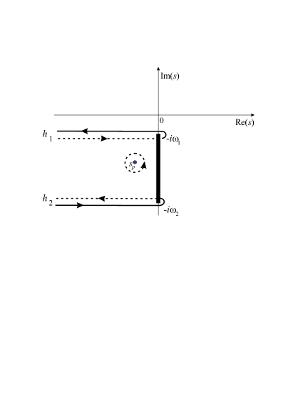
Figure 2: Integration contour used to calculate the inverse Laplace transform of $\hat{c}_{a}(s)$. The bold solid line on the imaginary axis is the branch cut. The integration along the solid (dashed) curves is made on the first (second) Riemannian sheet of $\hat{c}_{a}(s)$. $s_{p}$ is the pole of $\hat{c}_{a}(s)$ on the second Riemannian sheet in the ${\rm Re}(s)<0$ half-plane.

i.e.

$$-i\gamma_{p}+\Delta_{p}-\int_{\omega_{1}}^{\omega_{2}}d\omega\frac{\mathcal{D}(\omega)}{\omega_{a}+\Delta_{p}-i\gamma_{p}-\omega}+$$

$$+2\pi i\mathcal{D}(\omega_{a}+\Delta_{p}-i\gamma_{p})=0$$ (25)

where we have set

$$s_{p}\equiv-\gamma_{p}-i\omega_{a}-i\Delta_{p}.$$ (26)

After inversion, we then find for $c_{a}(t)$ the following decay law

$$c_{a}(t)=\mathcal{Z}\exp[-\gamma_{p}t-i(\omega_{a}+\Delta_{p})t]+\mathcal{C}(t),$$ (27)

where $\mathcal{Z}$ is the residue of $\hat{c}_{a}^{II}(s)$ at the pole $s_{p}$, and $\mathcal{C}(t)$ is the contribution from the contour integration along the Hankel paths $h_{1}$ and $h_{2}$ (see Fig.2):

$$\mathcal{C}(t) = \frac{1}{2\pi i}\int_{s=-\infty-i\omega_{1}}^{s=0-i\omega_{1}}ds\left[\hat{c}_{a}^{II}(s)-\hat{c}_{a}(s)\right]\exp(st)+$$ (28)

$$- \frac{1}{2\pi i}\int_{s=-\infty-i\omega_{2}}^{s=0-i\omega_{2}}ds\left[\hat{c}_{a}^{II}(s)-\hat{c}_{a}(s)\right]\exp(st).$$

The cut contribution $\mathcal{C}(t)$ is responsible for the appearance of non-exponential features in the decay dynamics, especially at short and long times; for an extensive and detailed analysis we refer the reader to e.g. Refs.Nakazato96 ; Regola ; examples of non-exponential decays will be presented in Sec.IV. We just mention here that, in the weak coupling limit ($\mathcal{D}\rightarrow 0$), from Eq.(25) one has that $\gamma_{p}$ and $\Delta_{p}$ are small, and thus using Eq.(19) we can cast Eq.(25) in the form

$$-i\gamma_{p}+\Delta_{p}-\mathcal{P}\int_{\omega_{1}}^{\omega_{2}}d\omega\frac{\mathcal{D}(\omega)}{\omega_{a}-\omega}+\pi i\mathcal{D}(\omega_{a})\simeq 0$$ (29)

from which we recover for the decay rate $\gamma_{p}$ and frequency shift $\Delta_{p}$ of the resonance the same expressions $\gamma_{R}$ and $\Delta_{R}$ as given by Eqs.(11) and (12) in the framework of the Weisskopf-Wigner analysis. In the strong coupling regime, close to the boundary of appearance of bound modes, the decay strongly deviates from an exponential law at any time scale, with the appearance of typical damped Rabi oscillations (see e.g. Ref. Tannoudji , pp. 249-255).

III.2 Microcavity with gain: lasing condition

Let us now consider the case of a microcavity with gain, i.e. $g^{\prime}>0$. In this case, one (or more) poles $s_{p}$ of $\hat{c}_{a}(s)$ on the first Riemannian sheet with ${\rm Re}(s)\geq 0$ may appear as the modal gain $g^{\prime}$ is increased, so that the mode amplitude $c_{a}(t)$ will grow with time, indicating the onset of an instability. In this case, the Bromwich path ${\rm B}$ should be closed taking into account the existence of one (or more than one) pole in the ${\rm Re}(s)\geq 0$ plane, as shown in Fig.3. For the case of a simple pole $s_{p}=-\gamma_{p}-i\omega_{a}-i\Delta_{p}$, the expression (27) for the temporal evolution of $c_{a}(t)$ is therefore still valid, where now $\gamma_{p}\leq 0$ and $\Delta_{p}$ are found as a solution of the equation [compare with Eq.(25)]

$$-i\gamma_{p}-ig^{\prime}+\Delta_{p}-\int_{\omega_{1}}^{\omega_{2}}d\omega\frac{\mathcal{D}(\omega)}{\omega_{a}+\Delta_{p}-i\gamma_{p}-\omega}=0.$$ (30)

Figure 3: (a) Deformation of the Bromwich path for inverse Laplace transformation with one pole $s_{p}$ on the ${\rm Re}(s)>0$ half-plane (unstable state). (b) Corresponding integration contour used to calculate the inverse Laplace transform. The integration along the solid (dashed) curves is made on the first (second) Riemannian sheet of $\hat{c}_{a}(s)$.

As a rather general rule, it turns out that, as $g^{\prime}$ is increased, the pole $s_{p}$ of $\hat{c}_{a}^{II}(s)$, which at $g^{\prime}=0$ lies in the ${\rm Re}(s)<0$ plane, crosses the imaginary axis in the cut region. This crossing changes the decay of $c_{a}(t)$ into a non-decaying or growing behavior, and thus it can be assumed as the threshold for laser oscillation. The modal gain at threshold, $g^{{}^{\prime}}_{th}$, is thus obtained from Eq.(30) by setting $\gamma_{p}=0^{-}$, i.e.

$$-ig^{{}^{\prime}}_{th}+\Delta_{p}-\Delta(\omega_{a}+\Delta_{p})+i\pi\mathcal{D}(\omega_{a}+\Delta_{p})=0,$$ (31)

where we used Eq.(21) and the relation

$$\int_{\omega_{1}}^{\omega_{2}}d\omega\frac{\mathcal{D}(\omega)}{\omega_{a}+\Delta_{p}+i0^{+}-\omega}=$$ (32)

$$=\mathcal{P}\int_{\omega_{1}}^{\omega_{2}}d\omega\frac{\mathcal{D}(\omega)}{\omega_{a}+\Delta_{p}-\omega}-i\pi\mathcal{D}(\omega_{a}+\Delta_{p}).$$ (33)

Therefore the threshold for laser oscillation is given by

$$g_{th}=\gamma_{i}+\pi\mathcal{D}(\omega_{a}+\Delta_{p}),$$ (34)

where $\Delta_{p}$ (the frequency shift of the oscillating mode from the microcavity resonance frequency $\omega_{a}$) is implicitly defined by the equation

$$\Delta_{p}=\mathcal{P}\int_{\omega_{1}}^{\omega_{2}}d\omega\frac{\mathcal{D}(\omega)}{\omega_{a}+\Delta_{p}-\omega},$$ (35)

i.e. $\Omega_{osc}-\omega_{a}=\Delta(\Omega_{osc})$ with $\Omega_{osc}=\omega_{a}+\Delta_{p}$. It should be noted that, under the conditions stated in Sec.III.A ensuring that for the passive microcavity no bound modes exist, Eq.(35) admits of (at least) one solution for $\omega_{a}+\Delta_{p}$ inside the range $(\omega_{1},\omega_{2})$. The simplest proof thereof can be done graphically [see Fig.1(a)] after observing that $\omega_{2}-\omega_{a}>\Delta(\omega_{2})$ and $\omega_{1}-\omega_{a}<\Delta(\omega_{1})$.
The rather simple Eq.(34) provides a generalization of Eq.(13) for the laser threshold of the active microcavity beyond the Markovian approximation and reduces to it in the limit $\Delta_{p}\simeq 0$. The frequency shift $\Delta_{p}$, however, can not be in general neglected and may strongly affect the value of $g_{th}$ in the strong coupling regime. In fact, for a small coupling of the microcavity with the structured reservoir ($\lambda\rightarrow 0$), the shift $\Delta_{p}$ can be neglected and therefore $g_{th}$ increases with $\lambda$ according to Eq.(13). However, as $\lambda$ is further increased up to the critical coupling condition, the shift $\Delta_{p}$ is no more negligible, and the oscillation frequency $\Omega_{osc}=\omega_{a}+\Delta_{p}$ at lasing threshold is pushed toward the boundaries $\omega_{1}$ or $\omega_{2}$, where $\mathcal{D}(\omega)$ and thus $g{{}^{\prime}}_{th}$ vanish. In fact, as $\lambda$ is increased to reach the minimum value between $\lambda_{I,II}$ defined by the relation note2 :

$$\lambda_{I,II}^{2}=(\omega_{1,2}-\omega_{a})\left[\mathcal{P}\int_{\omega_{1}}^{\omega_{2}}d\omega\frac{\sum_{\mu}|\kappa_{\mu}(\omega)|^{2}}{\omega_{1,2}-\omega}\right]^{-1},$$ (36)

one has $\Omega_{osc}\rightarrow\omega_{1,2}$, and hence $g_{th}\rightarrow\gamma_{i}$. Therefore, as $g_{th}$ initially increases from $\gamma_{i}$ as the coupling strength is increased from $\lambda=0$, it must reach a maximum value and then start to decrease until reaching again the $\gamma_{i}$ value as $\lambda$ approaches the critical value ($\lambda_{I}$ or $\lambda_{II}$). As the increase of $g_{th}$ with $\lambda$ in the weak coupling regime is simply understood as due to the acceleration of the decay of the microcavity mode into the neighboring waveguides, the successive decreasing of $g_{th}$ is related to the appearance of a back-coupling of the field from the continuum (waveguides) into the microcavity mode, until a bound state is formed at the critical coupling strength.
As a final remark, it should be noted that the precise dynamical features and the kind of instability at lasing threshold may depend on the specific structure function $\mathcal{D}(\omega)$ of the reservoir. In particular, anomalous dynamical features may occur at the critical coupling regime, as it will be shown in the next section.

IV An exactly-solvable model: the coupling of a microcavity with a coupled resonator optical waveguide

To clarify the general results obtained in the previous section, we present an illustrative example of exactly-solvable model in which a single-mode and high-$Q$ microcavity is tunneling-coupled to a CROW structure Stefanou98 ; Yariv99 ; Ozbay00 ; Olivier01 , which provides the non-markovian decay channel of the microcavity. In a CROW structure, photons tunnel from one evanescent defect mode of a cavity to the neighboring one due to overlapping between the tightly confined modes at each defect site, and therefore memory effects are expected to be non-negligible whenever the coupling rate of the microcavity with the CROW becomes comparable with the CROW hopping rate.

IV.1 The model

The schematic model of a microcavity tunneling-coupled to a CROW is shown in Fig.4 for two typical configurations. The CROW consists of a chain of equally-spaced optical waveguides Stefanou98 ; Yariv99 ; Ozbay00 ; Olivier01 , supporting a single band of propagating modes, and the microcavity is tunneling-coupled to either one [Fig.4(a)] or two [Fig.4(b)] cavities of the CROW. For the sake of definiteness, we will consider the coupling geometry shown in Fig.4(b), though similar results are obtained for the single-coupling configuration of Fig.4(a).

Figure 4: Schematic of a microcavity (M) tunneling-coupled to either one (a) or two (b) cavities of a coupled-resonator optical waveguide. Plot (c) shows a schematic of a microcavity coupled with a CROW in the configuration (b) realized on a PC planform made of a square lattice of air holes with a one-dimensional chain of defects patterned along the lattice (Ref.Liu05 ).

The microcavity and the CROW can be realized on a same PC planform (see, e.g., Liu05 ; Yanik04 ): the CROW is simply obtained by a one-dimensional periodic array of defects, placed at distance $d$ and patterned along the lattice to form resonant cavities with high-$Q$ factors. The microcavity is realized by one defect in the array, say the one corresponding to index $n=0$, which can have a resonance frequency $\omega_{a}$ different from that of adjacent defects and placed at a larger distance $d_{0}\geq d$ than the other cavities [see Fig.4(c)]. The CROW supports a continuous band of propagating modes whose dispersion relation, in the tight-binding approximation, is given by Yariv99

$$\omega(k)=\omega_{0}-2\kappa\cos(kd),$$ (37)

where $\kappa$ is the hopping amplitude between two consecutive cavities of the CROW, $d$ is the length of the unit cell of the CROW, $k$ is the Bloch wave number, and $\omega_{0}$ is the central frequency of the band. The resonance frequency $\omega_{m}$ of the microcavity is assumed to be internal to the CROW band, i.e. $\omega_{0}-2\kappa<\omega_{m}<\omega_{0}+2\kappa$. The microcavity is tunneling-coupled to the two adjacent cavities of the CROW, and we denote by $\kappa_{0}$ the hopping amplitude. The ratio $\kappa_{0}/\kappa$ and the position of $\omega_{m}$ inside the CROW band can be properly controlled by changing the geometrical parameters of the defects and the ratio $d_{0}/d$. In particular, in the limiting case where the microcavity has the same geometry and distance of the other CROW cavities, one has $\kappa_{0}=\kappa$ and $\omega_{m}=\omega_{0}$. An excellent and simple description of light transport in the system is provided by a set of coupled-mode equations for the amplitudes $a_{n}$ of modes in the cavities (see, e.g., Yariv99 ; Yanik04 )

$$i\dot{a}_{n} = -\kappa(a_{n+1}+a_{n-1})\;\;(|n|\geq 2)$$ (38a)

$$i\dot{a}_{-1} = -\kappa a_{-2}-\kappa_{0}c_{a}$$ (38b)

$$i\dot{c}_{a} = -\kappa_{0}(a_{-1}+a_{1})+(\omega_{a}+ig)c_{a}$$ (38c)

$$i\dot{a}_{1} = -\kappa a_{2}-\kappa_{0}c_{a}$$ (38d)

where $c_{a}$ is the amplitude of the microcavity mode, $g$ is its effective modal gain per unit time, and $\omega_{a}=\omega_{m}-\omega_{0}$ is the frequency detuning between the microcavity resonance frequency $\omega_{m}$ and the central frequency $\omega_{0}$ of the CROW band. For e.g. a CROW built in a GaAs-based PC with a square lattice of air holes in the design of Ref.Liu05 , a typical value of the cavity coupling coefficient turns out to be $\kappa\simeq 700-800$ GHz and $\omega_{0}/\kappa\sim 3\times 10^{3}$ at the $\lambda_{0}=850$ nm operation wavelength. Note that in writing Eqs.(38), we have neglected the internal losses of the CROW cavities; a reasonable value of the $Q$-factor for a realistic microcavity is $Q=\omega_{0}/(2\gamma_{loss})\sim 10^{6}$ Armani03 , which would correspond to a cavity loss rate $\gamma_{loss}\sim 1$ GHz to be added in Eqs.(38). This loss rate, however, is about two-to-three orders of magnitude smaller than the cavity coupling coefficient $\kappa$, and therefore on a short time scale non-Markovian dynamical effects should be observed even in presence of CROW losses. The effects of reservoir (CROW) losses will be briefly discussed at the end of the section.
To study the temporal evolution of an initial field in the microcavity, Eqs.(38) are solved with the initial condition $a_{n}(0)=0$ and $c_{a}(0)=1$. An integral representation for the solution of Eqs.(38) might be directly derived in the time domain by an extension of the technique described in Refs.Longhi06a ; Longhi06b , where a system of coupled-mode equations similar to Eqs.(38), but in the conservative (i.e. $g=0$) case, was considered. However, we prefer here to formally place Eqs.(38) into the more general Hamiltonian formalism of Sec.II and then use the Laplace transform analysis developed in the previous section to obtain the temporal evolution for $c_{a}(t)$. To this aim, in Appendix we prove that $c_{a}(t)$ may be obtained as a solution of the following equations, which have the canonical form (3) with a simple continuum of modes acting as a decay channel

$$i\dot{c}_{a}(t) = (\omega_{a}+ig)c_{a}+\lambda\int_{-2\kappa}^{2\kappa}d\omega\kappa_{\mu}(\omega)c(\omega,t)$$ (39a)

$$i\dot{c}(\omega,t) = \omega c(\omega,t)+\lambda\kappa_{\mu}(\omega)c_{a}(t)$$ (39b)

with

$$\lambda\kappa_{\mu}(\omega)=\kappa_{0}\sqrt{\frac{2}{\pi\kappa}}\left[1-\left(\frac{\omega}{2\kappa}\right)^{2}\right]^{1/4}.$$ (40)

Note that the reservoir structure function for this model, defined for $\omega_{1}<\omega<\omega_{2}$ with $\omega_{1}=-2\kappa$ and $\omega_{2}=2\kappa$, is simply given by

$$\mathcal{D}(\omega)=\frac{2\kappa_{0}^{2}}{\pi\kappa}\sqrt{1-\left(\frac{\omega}{2\kappa}\right)^{2}}.$$ (41)

With this reservoir structure function, the self-energy [Eq.(17)] can be calculated in an exact way and reads

$$\Sigma(s)=i\left(\frac{\kappa_{0}}{\kappa}\right)^{2}\left[s-\sqrt{4\kappa^{2}+s^{2}}\right].$$ (42)

The function $\Delta(\omega)$, as defined by Eq.(21), then reads

$$\Delta(\omega)=\left\{\begin{array}[]{lr}(\kappa_{0}/\kappa)^{2}\omega&|\omega|<2\kappa\\ (\kappa_{0}/\kappa)^{2}\left[\omega-\sqrt{\omega^{2}-4\kappa^{2}}\right]&\omega>2\kappa\\ (\kappa_{0}/\kappa)^{2}\left[\omega+\sqrt{\omega^{2}-4\kappa^{2}}\right]&\omega<-2\kappa\end{array}\right.$$ (43)

Note that the coupling strength between the microcavity and the CROW is determined by the ratio $\kappa_{0}/\kappa$, the limit $\kappa_{0}/\kappa\rightarrow 0$ corresponding to the weak coupling regime.

IV.2 The passive microcavity: from exponential decay to damped Rabi oscillations

Let us consider first the case $g=0$. The conditions for the non-existence of bound modes, i.e. for a complete decay of $c_{a}(t)$, are $\omega_{2}-\omega_{a}\geq\Delta(\omega_{2})$ and $\omega_{1}-\omega_{a}\leq\Delta(\omega_{1})$ (see Sec.III.A), which using Eq.(43) read explicitly

$$\left(\frac{\kappa_{0}}{\kappa}\right)^{2}-1\leq\frac{\omega_{a}}{2\kappa}\leq 1-\left(\frac{\kappa_{0}}{\kappa}\right)^{2}.$$ (44)

Note that, as a necessary condition, this relation implies that $|\omega_{a}|\leq 2\kappa$ and $(\kappa_{0}/\kappa)^{2}\leq 1$. Note also that the the critical coupling regime is reached at $(\kappa_{0}/\kappa)=\sqrt{1-|\omega_{a}|/(2\kappa)}$. For a coupling strength $(\kappa_{0}/\kappa)$ above such a value, the decay of $c_{a}(t)$ is imperfect due to the existence of bound modes between the microcavity and the CROW; this case will not be considered here further.
The temporal decay law for the mode amplitude $c_{a}(t)$ can be generally expressed using the general relation (27), which highlights the existence of the exponential (Weisskopf-Wigner) decaying term plus its correction due to the contribution of the Hankel paths. Perhaps, for the microcavity-CROW system it is more suited to make the inverse Laplace transform on the first Riemannian sheet of $\hat{c}_{a}(s)$ by closing the Bromwich path ${\rm B}$ with a semicircle with radius $R\rightarrow\infty$ in the ${\rm Re}(s)<0$ half-plane after excluding the branch cut from the domain by the contour $\sigma$ as shown in Fig.5. Since in this case there are no singularities of $\hat{c}_{a}(s)$, we simply obtain

$$c_{a}(t)=\frac{1}{2\pi}\oint_{\sigma}ds\;\frac{\exp(st)}{is-\omega_{a}-\Sigma(s)}$$ (45)

which, using Eq.(20), reads explicitly

Figure 5: Integration contour used for the inverse Laplace transform in the passive microcavity-CROW system.

$$c_{a}(t) = \frac{i}{2\pi}\int_{\omega_{1}}^{\omega_{2}}d\omega\left[\frac{\exp(-i\omega t)}{\omega-\omega_{a}-\Sigma(-i\omega+0^{+})}+\right.$$ (46)

$$- \left.\frac{\exp(-i\omega t)}{\omega-\omega_{a}-\Sigma(-i\omega-0^{+})}\right]=$$

$$= \int_{\omega_{1}}^{\omega_{2}}d\omega\frac{\mathcal{D}(\omega)\exp(-i\omega t)}{[\omega-\omega_{a}-\Delta(\omega)]^{2}+\pi^{2}\mathcal{D}^{2}(\omega)}.$$

For the microcavity-CROW model, one then obtains

$$c_{a}(t)=\frac{1}{2\pi}\frac{\kappa_{0}^{2}}{\kappa^{3}}\int_{-2\kappa}^{2\kappa}d\omega\frac{\exp(-i\omega t)\sqrt{1-(\omega/2\kappa)^{2}}}{\left\{(\omega/2\kappa)\left[1-(\kappa_{0}/\kappa)^{2}\right]-(\omega_{a}/2\kappa)\right\}^{2}+(\kappa_{0}/\kappa)^{4}[1-\omega^{2}/(4\kappa^{2})]}.$$ (47)

The integral on the right hand side in Eq.(47) can be written in a more convenient form with the change of variable $\omega=-2\kappa\cos Q$, yielding

$$c_{a}(t)=\frac{1}{\pi}\int_{0}^{\pi}dQ\frac{(k_{0}/\kappa)^{2}\sin^{2}Q\exp(2i\kappa t\cos Q)}{\left[(\omega_{a}/2\kappa)+\cos Q-(\kappa_{0}/\kappa)^{2}\cos Q\right]^{2}+(\kappa_{0}/\kappa)^{4}\sin^{2}Q}.$$ (48)

In this form, the integral can be written Longhi06a as a series of Bessel functions of first kind and of argument $2\kappa t$ (Neumann series). Special cases, for which a simple expression for $c_{a}(t)$ is available, are those corresponding to $\omega_{a}=0$ and $\kappa_{0}=\kappa$, for which

$$c_{a}(t)=J_{0}(2\kappa t),$$ (49)

and to $\omega_{a}=0$ and $\kappa_{0}=\kappa/\sqrt{2}$, for which

$$c_{a}(t)=\frac{J_{1}(2\kappa t)}{\kappa t}.$$ (50)

Note that the former case corresponds to a critical coupling regime, where $\hat{c}_{a}(s)$ has two singularities at $s=\pm 2i\kappa+0^{+}$. The residues of $\hat{c}_{a}(s)$ at these singularities, however, vanish, and therefore the field $c_{a}(t)$ fully decays toward zero with an asymptotic power law $\sim 1/t^{1/2}$. In general, an inspection of the singularities of the $\hat{c}_{a}(s)$ reveals that, for $\omega_{a}\neq 0$, at the critical coupling strength $(\kappa_{0}/\kappa)=\sqrt{1-|\omega_{a}|/(2\kappa)}$ the Laplace transform $\hat{c}_{a}(s)$ has one singularity at either $s_{p}=2i\kappa+0^{+}$ or $s_{p}=-2i\kappa+0^{+}$ of type $\hat{c}_{a}(s)\sim 1/\sqrt{s-s_{p}}$.
The asymptotic decay behavior of $c_{a}(t)$ at long times can be determined by the application of the method of the stationary phase to Eq.(48). One then finds that at the critical coupling the field $c_{a}(t)$ decays toward zero with an asymptotic power law $\sim 1/t^{1/2}$, whereas below the critical coupling the decay is faster with an asymptotic decay $\sim 1/t^{3/2}$.
Typical examples of non-exponential features in the decay process as the coupling strength is increased are shown in Fig.6 for $\omega_{a}=0$. The curves in the figures have been obtained by a direct numerical solution of Eqs.(38). Note that, as for weak coupling the exponential (Weisskopf-Wigner) decay law is retrieved with a good approximation [see Fig.6(a)], as the coupling strength $\kappa_{0}/\kappa$ is increased the decay law strongly deviates from an exponential behavior. Note in particular the existence of strong oscillations, which are fully analogous to damped Rabi oscillations found in the atom-photon interaction context Tannoudji . For $\omega_{0}\neq 0$, the oscillatory behavior of the long-time power-law decay is less pronounced and may even disappear (see Ref.Longhi06a ).

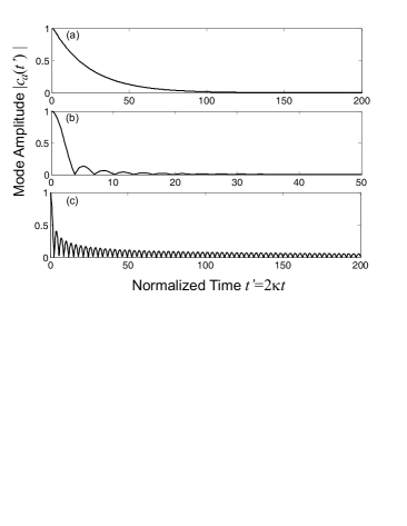
Figure 6: Decay of the mode amplitude $|c_{a}(t)|$ in a passive microcavity-CROW system for $\omega_{a}=0$ and for increasing values of coupling strength: (a) $\kappa_{0}/\kappa=0.2$, (b) $\kappa_{0}/\kappa=0.707$, and (c) $\kappa_{0}/\kappa=1$ (critical coupling).

IV.3 Microcavity with gain

Let us consider now the case $g\geq 0$. In order to determine the threshold for laser oscillation, we have to distinguish three cases depending on the value of the coupling strength $\kappa_{0}/\kappa$.

(i) Lasing condition below the critical coupling. In this case, corresponding to $\kappa_{0}/\kappa<\sqrt{1-|\omega_{a}|/(2\kappa)}$, the threshold for laser oscillation is readily obtained from Eqs.(34), (35), (41) and (43). The frequency $\Omega_{osc}$ of the oscillating mode is given by $\Omega_{osc}=\omega_{a}/[1-(\kappa_{0}/\kappa)^{2}]$, and the gain for laser oscillation is thus given by

$$g_{th}=2\kappa\left(\frac{\kappa_{0}}{\kappa}\right)^{2}\sqrt{1-\left[\frac{\omega_{a}/(2\kappa)}{1-(\kappa_{0}/\kappa)^{2}}\right]^{2}}.$$ (51)

The typical behavior of normalized threshold gain $g_{th}/(2\kappa)^{2}$ versus the coupling strength $(\kappa_{0}/\kappa)$ is shown in Fig.7.

Figure 7: Behavior of normalized threshold gain $g_{th}/(2\kappa)$ versus the coupling strength $(\kappa_{0}/\kappa)^{2}$ for a few values of the ratio $\omega_{a}/(2\kappa)$.

Note that, according to the general analysis of Sec.III.B, the threshold for laser oscillation first increases as the coupling strength is increased, but then it reaches a maximum and then decreases toward zero as the critical coupling strength is attained. At $g=g_{th}$, $\hat{c}_{a}(s)$ has a simple pole at $s=s_{p}=-i\Omega_{osc}+0^{+}$, whereas as $g$ is increased above $g_{th}$ the pole $s_{p}$ invades the ${\rm Re}(s)>0$ half-plane. Therefore, the onset of lasing is characterized by an amplitude $|c_{a}(t)|$ which asymptotically decays toward zero for $g<g_{th}$, reaches a steady-state and nonvanishing value at $g=g_{th}$ (the field does not decay nor grow asymptotically), whereas it grows exponentially (in the early lasing stage) for $g>g_{th}$ with a growth rate $\sigma(g)={\rm Re}(s_{p})$ (see Fig.8). This instability scenario is the usual one encountered in the semiclassical theory of laser oscillation as a second-order phase transition note3 . However, the temporal dynamics at the onset of lasing shows unusual oscillations [see Fig.8(a)] which are a signature of non-Markovian dynamics. In addition, as in the Markovian limit the growth rate $\sigma$ should increase linearly with $g-g_{th}$, in the strong coupling regime the growth rate $\sigma$ shows near threshold an unusual non-linear behavior, as shown in Fig.8(b).

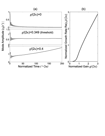
Figure 8: (a) Behavior of mode amplitude $|c_{a}(t^{\prime})|$ versus normalized time $t^{\prime}=2\kappa t$ for $(\kappa_{0}/\kappa)^{2}=0.8$, $\omega_{a}/(2\kappa)=0.18$, and for increasing values of normalized gain $g/(2\kappa)$. (b) Behavior of normalized growth rate versus normalized gain for $(\kappa_{0}/\kappa)^{2}=0.8$ and $\omega_{a}/(2\kappa)=0.18$.

(ii) Lasing condition at the critical coupling with $\omega_{a}\neq 0$. A different dynamics occurs when the coupling strength $\kappa/\kappa_{0}$ reaches the critical limit $\kappa_{0}/\kappa=\sqrt{1-|\omega_{a}|/(2\kappa)}$. As discussed in Sec.IV.B, at $g=0$ the Laplace transform $\hat{c}_{a}(s)$ has a singularity at either $s_{p}=2i\kappa$ or $s_{p}=-2i\kappa$, however $s_{p}$ is not a simple pole and $c_{a}(t)$ asymptotically decays toward zero. For $\omega_{a}\neq 0$, i.e. for $(\kappa/\kappa_{0})<1$, as $g$ is increased just above zero $\hat{c}_{a}(s)$ shows a simple pole with a growth rate $\sigma={\rm Re}(s_{p})>0$ which slowly increases with $g$ at the early stage, as shown in Fig.9. In the figure, a typical temporal evolution of $c_{a}(t)$ is also shown. Note that in this case there is not a value of $g$ for which the field amplitude $c_{a}(t)$ does not grow nor decay, i.e. the intermediate situation shown in Fig.8(a) is missed in Fig.9(a): for $g=0$ the amplitude decays, however for $g=0^{+}$ it always grows exponentially. The transition describing the passage of laser from below to above threshold in the linear stage of the instability is therefore quite unusual at the critical coupling.

Figure 9: Same as Fig.8, but for parameter values $(\kappa_{0}/\kappa)^{2}=0.8$ and $\omega_{a}/(2\kappa)=0.2$ (critical coupling). Note that in this case there exists no lasing threshold in the traditional sense.

(iii) Lasing condition at the critical coupling with $\omega_{a}=0$. A somewhat singular behavior occurs at the critical coupling when $\omega_{a}=0$, and therefore $\kappa_{0}/\kappa=1$. This case corresponds to consider a periodic CROW in which one of the cavities is pumped and acts as the microcavity in our general model. For $\omega_{a}=0$ and $\kappa_{0}/\kappa=1$, the Laplace transform $\hat{c}_{a}(s)$ is explicitly given by

$$\hat{c}_{a}(s)=\frac{1}{-g+\sqrt{s^{2}+4\kappa^{2}}}.$$ (52)

To perform the inversion, one needs to distinguish four cases.
(a) $g=0$. For $g=0$, the field $c_{a}(t)$ decays according to

$$c_{a}(t)=J_{0}(2\kappa t)$$ (53)

as shown in Sec.IV.B.

(b) $0<g<2\kappa$. In this case $\hat{c}_{a}(s)$ has two simple poles on the first Riemannian sheet at $s_{1,2}=\pm i\sqrt{4\kappa^{2}-g^{2}}+0^{+}$. The inversion can be performed by closing the Bromwich path ${\rm B}$ with the contour shown in Fig.10, where along the dashed curves the integrals are performed on the second Riemannian sheet. One then obtains

$$c_{a}(t)=\frac{2g}{\sqrt{4\kappa^{2}-g^{2}}}\sin\left(\sqrt{4\kappa^{2}-g^{2}}t\right)+\mathcal{C}(t)$$ (54)

where the first term on the right hand side in the equation arises from the residues at poles $s_{1,2}$, whereas $\mathcal{C}(t)$ is the contribution from the contour integration along the Hankel paths $h_{1}$ and $h_{2}$, which asymptotically decays toward zero as $t\rightarrow\infty$. Note that, after an initial transient, the amplitude $|c_{a}(t)|$ steadily oscillates in time with frequency $\sqrt{4\kappa^{2}-g^{2}}$ and amplitude $2g/\sqrt{4\kappa^{2}-g^{2}}$. Note also that the amplitude and period of oscillations diverge as the modal gain $g$ approaches $2\kappa^{-}$.

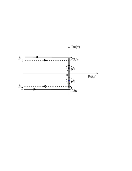
Figure 10: Integration contour used to calculate the inverse Laplace transform for $\omega_{a}=0$, $\kappa_{0}/\kappa=1$ and for $0<g/(2\kappa)<1$. The integration along the solid (dashed) curves is made on the first (second) Riemannian sheet of $\hat{c}_{a}(s)$. $s_{1,2}$ are the two poles of $\hat{c}_{a}(s)$ on the imaginary axis inside the cut.

(c) $g=2\kappa$. In this case, $\hat{c}_{a}(s)$ has a single pole of second-order in $s=0^{+}$, and therefore to perform the inversion it is worth separating the singular and non-singular parts of $\hat{c}_{a}(s)$ as

$$\hat{c}_{a}(s)=\frac{4\kappa}{s^{2}}+f(s)$$ (55)

where $f(s)$ has no singularities on the imaginary axis. After inversion one then obtains

$$c_{a}(t)=4\kappa t+\frac{1}{2\pi}\int_{-\infty}^{\infty}d\omega\;f(-i\omega+0^{+})\exp(-i\omega t),$$ (56)

where the second term on the right-hand side in the above equation asymptotically decays toward zero. Therefore, we may conclude that at $g=2\kappa$ the mode amplitude $c_{a}(t)$ is dominated by a secular growing term which is not exponential.

(d) $g>2\kappa$. In this case, $\hat{c}_{a}(s)$ has an unstable simple pole at $s_{p}=(g^{2}-4\kappa^{2})^{1/2}$, and therefore the solution $c_{a}(t)$ grows exponentially with time.

The dynamical scenario described above for $\omega_{a}=0$ and $\kappa_{0}/\kappa=1$ is illustrated in Fig.11. Note that in this case there is some uncertainty in the definition of laser threshold, since there exists an entire interval of modal gain values, from $g=0^{+}$ to $g=2\kappa^{-}$, at which an initial field in the cavity does not grow nor decay.

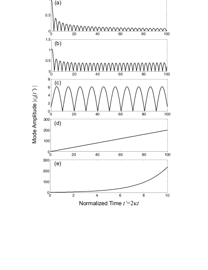
Figure 11: Behavior of mode amplitude $c_{a}(t^{\prime})$ versus normalized time $t^{\prime}=2\kappa t$ for $\omega_{a}=0$, $\kappa_{0}/\kappa=1$ (critical coupling) and for increasing values of normalized gain: (a) $g/(2\kappa)=0$, (b) $g/(2\kappa)=0.2$, (c) $g/(2\kappa)=0.95$, (d) $g/(2\kappa)=1$, and (d) $g/(2\kappa)=1.1$.

As a final comment, we briefly discuss the effects of internal losses of the CROW cavities, which have been so far neglected, on the temporal evolution of the mode amplitude $c_{a}(t)$. In the case where all the cavities in the CROW have the same loss rate $\gamma_{loss}$, the temporal evolution of $c_{a}(t)$ is simply modified by the introduction of an additional exponential damping factor $\exp(-\gamma_{loss}t)$, i.e. $c_{a}(t)\rightarrow c_{a}(t)\exp(-\gamma_{loss}t)$. This additional decay term would therefore shift the threshold for laser oscillation to higher values and, most importantly for our analysis, it might hinder non-Markovian dynamical effects discussed so far. However, for a small value of $\gamma_{loss}/\kappa$ (e.g. $\gamma_{loss}/\kappa\sim 0.01$ for the numerical values given in Ref.Liu05 ), non-Markovian effects should be clearly observable in the transient field dynamics for times shorter than $\sim 1/\gamma_{loss}$. As an example, Fig.12 shows the dynamical evolution of the mode amplitude $|c_{a}(t)|$ for the same parameter values of Fig.11, except for the inclusion of a CROW loss rate $\gamma_{loss}=0.01\kappa$. It is worth commenting on the dynamical behavior of Fig.12(d) corresponding to $g=2\kappa$. In this case, using Eq.(56) and disregarding the decaying term on the right hand side in Eq.(56), one can write

$$c_{a}(t)\sim 4\kappa t\exp(-\gamma_{loss}t).$$ (57)

Note that in the early transient stage the initial mode amplitude stored in the microcavity linearly grows as in Fig.11(d), however it reaches a maximum and then it finally decays owing to the prevalence of the loss-induced exponential term over the linear growing term. Therefore, though the microcavity is below threshold for oscillation as an initial field in the cavity asymptotically decays to zero, before decaying an initial field is subjected to a transient amplification. The maximum amplification factor in the transient is about $\sim 2\kappa/\gamma_{loss}$, and can be therefore relatively large in high-$Q$ microcavities. Such a transient growth despite the asymptotic stability of the zero solution should be related to the circumstance that for $g\neq 0$ the system (38) is non-normal note4 : though its eigenvalues have all a negative real part, the system can sustain a transient energy growth. The transient amplification shown in Fig.12(d) is therefore analogous to non-normal energy growth encountered in other hydrodynamic Trefethen93 ; Farrell94 ; Farrell96 and optical Kartner99 ; Longhi00 ; Firth05 systems and it is an indicator of a major sensitivity of the system to noise.

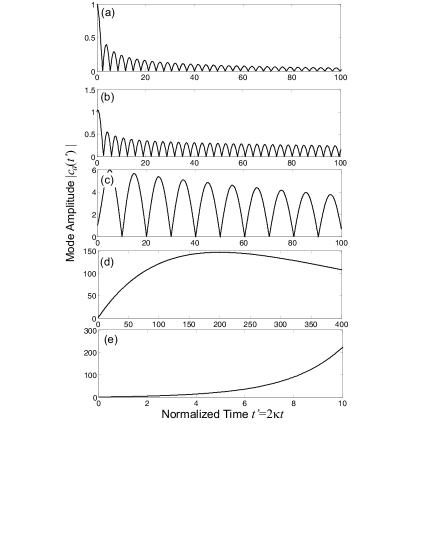
Figure 12: Same as Fig.11, but in presence of CROW losses ($\gamma_{loss}/\kappa=0.01$).

V Conclusions

In this work it has been analytically studied, within a rather general Hamiltonian model [Eqs.(1)], the dynamics of a classical field in a single-mode optical microcavity coupled to a structured continuum of modes (reservoir) beyond the usual Weisskopf-Wigner (Markovian) approximation. Typical non-Markovian effects for the passive microcavity are non-exponential decay and damped Rabi oscillations (Sec.III.A). In presence of gain, the general condition for laser oscillation, that extends the usual gain/loss rate balance condition of elementary laser theory, has been derived (Sec.III.B), and the behavior of the laser threshold versus the microcavity-reservoir coupling has been determined. The general results have been specialized for an exactly-solvable model, which can be implemented in a photonic crystal with defects: an optical microcavity tunneling-coupled to a coupled-resonator optical waveguide (Sec.IV). A special attention has been devoted to study the transition describing laser oscillation at the critical coupling between the cavity and the waveguide (Sec.IV.C). Unusual dynamical effects, which are a clear signature of a non-Markovian dynamics, have been illustrated, including: the existence of a finite interval of modal gain where the field oscillates without decaying nor growing, the gain parameter controlling the amplitude and period of the oscillations; a linear (instead of exponential) growth of the field at the onset of instability for laser oscillation; and the existence of transient (non-normal) amplification of the field below laser threshold when intrinsic losses of the microcavity are considered. It is envisaged that, though non-Markovian effects are not relevant in standard laser resonators in which the field stored in the cavity is coupled to the broad continuum of modes of the external open space by a partially-transmitting mirror Lang73 , they should be observable when dealing with high-$Q$ microcavities coupled to waveguides, which act as a structured decay channel for the field stored in the microcavity.

Appendix A

In this Appendix it is proved the equivalence between coupled-mode equations (38) in the tight-binding approximation and the canonical formulation for the decay of a discrete state into a continuum provided by Eqs.(39). To this aim, let us first note that, owing to the inversion-symmetry of the initial condition $a_{-n}(0)=a_{n}(0)=0$ ($n\neq 0$), it can be readily shown that the solution $a_{n}(t)$ maintains the same symmetry at any time, i.e. $a_{-n}(t)=a_{n}(t)$ for $t\geq 0$. Let us then introduce the continuous function of the real-valued parameter $Q$

$$\phi(Q,t)=\sum_{n=1}^{\infty}a_{n}(t)\sin(nQ),$$ (58)

where $Q$ is taken inside the interval $[0,\pi]$. Using the relation

$$\int_{0}^{\pi}dQ\;\sin(nQ)\sin(mQ)=\frac{\pi}{2}\delta_{m,n}\;\;\;(m,n\geq 1)$$ (59)

the amplitudes $a_{n}$ of modes in the CROW are related to the continuous field $\phi$ by the simple relations

$$a_{n}(t)=\frac{2}{\pi}\int_{0}^{\pi}dQ\;\phi(Q,t)\sin(nQ)$$ (60)

($n\geq 1$). The equation of motion for $\phi$ is readily obtained from Eqs.(38) and reads

$$i\frac{\partial\phi}{\partial t}=-2\kappa\cos(Q)\phi-\kappa_{0}\sin(Q)c_{a}$$ (61)

whereas the equation for $c_{a}$, taking into account that $a_{-1}+a_{1}=2a_{1}=(4/\pi)\int_{0}^{\pi}dQ\phi(Q,t)\sin(Q)$, can be cast in the form:

$$i\dot{c}_{a}(t)=(\omega_{a}+ig)c_{a}(t)-\frac{4\kappa_{0}}{\pi}\int_{0}^{\pi}dQ\;\phi(Q,t)\sin(Q).$$ (62)

By introducing the frequency $\omega$ of the continuum

$$\omega=-2\kappa\cos(Q)$$ (63)

and after setting

$$c(\omega,t)=-\sqrt{\frac{2}{\pi\kappa}}\phi(\omega,t)\frac{1}{\left[1-\omega^{2}/(2\kappa)^{2}\right]^{1/4}},$$ (64)

one finally obtains Eqs.(39a) and (39b) given in the text.

References

- (1) R. Lang, O. Scully, and W.E. Lamb, Phys. Rev. A 7, 1788 (1973).
- (2) S.C. Ching, H.M. Lai, and K. Young, J. Opt. Soc. Am. B 4, 1995 (1987).
- (3) E.S.C. Ching, P.T. Leung, A. Maassen van den Brink, W.M. Suen, S.S. Tong, and K. Young, Rev. Mod. Phys. 70, 1545 (1998).
- (4) U. Fano, Phys Rev.124, 1866 (1961).
- (5) C. Cohen-Tannoudji, J. Dupont-Roc, and G. Grynberg, Atom-Photon Interactions (Wiley, New York, 1992).
- (6) O. Svelto, Principles of Lasers, fourth ed. (Springer, Berlin, 1998).
- (7) It is remarkable as well that the usual gain/loss balance condition for lasing threshold, with an exponential growth at the onset of lasing, is valid even for less conventional laser systems, such as in random lasers [see, for instance: V. S. Letokhov, Sov. Phys. JETP 26, 835 (1968); T. Sh. Misirpashaev and C.W.J. Beenakker, Phys. Rev. A 57, 2041 (1998); X. Jiang and C.M. Soukoulis, Phys. Rev. B 59, 6159 (1999); A.L. Burin, M.A. Ratner, H. Cao, and S.H. Chang, Phys. Rev. Lett. 88, 093904 (2002)].
- (8) B. Piraux, R. Bhatt, and P.L. Knight, Phys. Rev. A 41, 6296 (1990).
- (9) H.M. Lai, P.T. Leung, and K. Young, Phys. Rev. A 37, 1597 (1988).
- (10) M. Lewenstein, J. Zakrzewski, T.W. Mossberg, and J. Mostowski, J. Phys. B: At. Mol. Opt. Phys. 21, L9 (1988).
- (11) S. John and J. Wang, Phys. Rev. Lett. 64, 2418 (1990).
- (12) S. John and T. Quang, Phys. Rev. A 50, 1764 (1994).
- (13) A.G. Kofman, G. Kurizki, and B. Sherman, J. Mod. Opt. 41, 353 (1994).
- (14) N. Vats and S. John, Phys. Rev. A 58, 4168 (1998).
- (15) P. Lambropoulos, G.M. Nikolopoulos, T.R. Nielsen, and S. Bay, Rep. Prog. Phys. 63, 455 (2000).
- (16) X.-H. Wang, B.-Y. Gu, R. Wang, and H.-Q. Xu, Phys. Rev. Lett. 91, 113904 (2003).
- (17) T. Petrosky, C.-O. Ting, and S. Garmon, Phys. Rev. Lett. 94, 043601 (2005).
- (18) S. Tanaka, S. Garmon, and T. Petrosky, Phys. Rev. B 73, 115340 (2006).
- (19) B. Gaveau and L.S. Schulman, J. Phys. A: Math. Gen. 28, 7359 (1995).
- (20) P.R. Villeneuve, S. Fan, and J.D. Joannopoulos, Phys. Rev. B 54, 7837 (1996).
- (21) K.J. Vahala, Nature (London) 424, 839 (2003).
- (22) D.K. Armani, T.J. Kippenberg, S.M. Spillane, and K.J. Vahala, Nature (London) 421, 925 (2003).
- (23) T. Asano and S. Noda, Nature (London) 429, 6988 (2004).
- (24) T. Asano, W. Kunishi, B.-S. Song, and S. Noda, Appl. Phys. Lett. 88, 151102 (2006).
- (25) O. Painter, R. K. Lee, A. Yariv, A. Scherer, J. D. O Brien, P. D. Dapkus, and I. Kim, Science 284, 1819 (1999).
- (26) M. Loncar, T. Yoshie, A. Scherer, P. Gogna, and Y. Qiu, Appl. Phys. Lett. 81, 2680 (2002).
- (27) H.G. Park, S.H. Kim, S.H. Kwon, Y.G. Ju, J.K. Yang, J.H. Baek, S.B. Kim, and Y.H. Lee, Science 305, 1444 (2004).
- (28) H. Altug and J. Vuckovic, Opt. Express 13, 8819 (2005).
- (29) S. Fan, P.R. Villeneuve, J.D. Joannopoulos, and H.A. Haus, Phys. Rev. Lett. 80, 960 (1998); S. Fan, P.R. Villeneuve, J.D. Joannopoulos, M.J. Khan, C. Manolatou, and H.A. Haus, Phys. Rev. B 59, 15882 (1999).
- (30) Y. Xu, Y. Li, R.K. Lee, and A. Yariv, Phys. Rev. E 62, 7389 (2000).
- (31) T. Asano, B.S. Song, Y. Tanaka, and S. Noda, Appl. Phys. Lett. 83, 407 (2003).
- (32) E. Waks and J. Vuckovic, Opt. Express 13, 5064 (2005).
- (33) P. Chak, S. Pereira, and J.E. Sipe, Phys. Rev. B 73, 035105 (2006).
- (34) M.F. Yanik and S. Fan, Phys. Rev. A 71, 013803 (2005).
- (35) L.-L. Lin, Z.-Y. Li, and B. Lin, Phys. Rev. B 72, 165330 (2005).
- (36) N. Stefanou and A. Modinos, Phys. Rev. B 57, 12127 (1998).
- (37) A. Yariv, Y. Xu, R.K. Lee, and A. Scherer, Opt. Lett. 24, 711 (1999).
- (38) M. Bayindir, B. Temelkuran, and E. Ozbay, Phys. Rev. Lett. 84, 2140 (2000).
- (39) S. Olivier, C. Smith, M. Rattier, H. Benisty, C. Weisbuch, T. Krauss, R. Houdre, and U. Oesterle, Opt. Lett. 26, 1019 (2001).
- (40) Y. Liu, Z. Wang, M. Han, S. Fan, and R. Dutton, Opt. Express 13, 4539 (2005).
- (41) H. Nakazato, M. Namiki, and S. Pascazio, Int. J. Mod. Phys. B 10, 247 (1996).
- (42) P. Facchi and S. Pascazio, La Regola d’Oro di Fermi, in: Quaderni di Fisica Teorica, edited by S. Boffi (Bibliopolis, Napoli, 1999).
- (43) Note that, by extending the definition of outside the interval , the principal value of the integral in Eq.(21) can be removed.
- (44) The value () defines the critical value of coupling strenght above which a bound mode (discrete eigenvalue of ) at frequency () appears.
- (45) M.F. Yanik and S. Fan, Phys. Rev. Lett. 92, 083901 (2004).
- (46) S. Longhi, Phys. Rev. E 74, 026602 (2006).
- (47) S. Longhi, Phys. Rev. Lett. 97, 110402 (2006).
- (48) If gain saturation is accounted for and the dynamics may be derived from a potential (e.g. after adiabatic elimination of polarization and population inversion in the semiclassical laser equations), the onset of laser oscillation is analogous to a second-order phase transition [see, for instance: V. DeGiorgio and M.O. Scully, Phys. Rev. A 2, 1170 (1970); H. Haken, Synergetics, second ed. (Springler-Verlag, Berlin, 1978)].
- (49) Denoting by the matrix for the linear system (38) of ordinary differential equations, the system is referred to as non-normal whenever does not commute with its adjoint . One can show that transient energy amplification is possible in an asymptotically-stable non-normal system provided that the largest eigenvalue of is positive (see e.g. Farrell96 ). Non-hermiticity is a necessary (but not sufficient) condition to have transient energy grow in an asymptotically-stable linear system.
- (50) L.N. Trefethen, A.E. Trefethen, S.C. Reddy, and T.A. Driscoll, Science 261, 578 (1993).
- (51) B.F. Farrell and P.J. Ioannou, Phys. Rev. Lett. 72, 1188 (1994).
- (52) B. F. Farrell and P.J. Ioannou, J. Atmos. Sci. 53, 2025 (1996).
- (53) F.X. Kärtner, D.M. Zumbühl, and N. Matuschek, Phys. Rev. Lett. 82, 4428 (1999).
- (54) S. Longhi and P. Laporta, Phys. Rev. E 61, R989 (2000).
- (55) W.J. Firth and A.M. Yao, Phys. Rev. Lett. 95, 073903 (2005).