Traceable 2D finite-element simulation of the whispering-gallery modes of axisymmetric electromagnetic resonators

Abstract

This paper explains how a popular, commercially-available software package for solving partial-differential-equations (PDEs), as based on the finite-element method (FEM), can be configured to calculate, efficiently, the frequencies and fields of the whispering-gallery (WG) modes of axisymmetric dielectric resonators. The approach is traceable; it exploits the PDE-solver’s ability to accept the definition of solutions to Maxwell’s equations in so-called ‘weak form’. Associated expressions and methods for estimating a WG mode’s volume, filling factor(s) and, in the case of closed(open) resonators, its wall(radiation) loss, are provided. As no transverse approximation is imposed, the approach remains accurate even for quasi-transverse-magnetic/electric modes of low, finite azimuthal mode order. The approach’s generality and utility are demonstrated by modeling several non-trivial structures: (i) two different optical microcavities [one toroidal made of silica, the other an AlGaAs microdisk]; (ii) a 3rd-order sapphire:air Bragg cavity; (iii) two different cryogenic sapphire WG-mode resonators; both (ii) and (iii) operate in the microwave X-band. By fitting one of (iii) to a set of measured resonance frequencies, the dielectric constants of sapphire at liquid-helium temperature have been estimated.

I Introduction

Non-trivial electromagnetic structures can be modeled through computer-aided design (CAD) tools in conjunction with programs for numerically solving Maxwell’s equations. Though alternatives abound [1, 2, 3], the latter often use the finite-element method (FEM) [4, 5]. Within such a scheme, a problem frequently encountered when attempting to determine the values of electromagnetic parameters from experimental data is a lack of traceability: significant dependencies between the data, the model’s configurational settings, and the inferred values of parameters cannot be adequately isolated, understood, or quantified. Traceability demands that both the model’s definition and its solution remain amenable to complete, explicit description. And, furthermore, convenience requires that the representations adopted for this purpose be concise –yet wholly unambiguous.

I-A Whispering-gallery-mode resonators

Certain compact electromagnetic structures support closed whispering-gallery (WG) modes. Though elliptical [6] or even non-planar (‘crinkled’ [7] or ‘spooled’ [8]) WG morphologies exhibit advantageous features with respect to certain applications, this paper considers only (closed, planar) WG modes with circular trajectories, as supported by axisymmetric resonators within the class depicted in Fig. 1, upon which various recent scientific innovations [9, 10, 11, 12] are based.

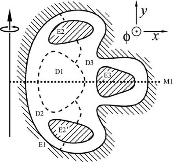
Figure 1: Generic axisymmetric resonator in cross-section (medial half-plane). A dielectric volume (in 3D) or ‘domain’ (in 2D) is enclosed by an electric wall (E1) –or one subject to some different boundary condition, as per subsubsection III-E2. This domain comprises several subdomains (D1, D2, and D3), each containing a spatially uniform dielectric (that could be just free space). Some of these subdomains (D2 and D3) are bounded internally by electric walls (E2, E2^′ and E3). The resonator has (optionally) a mirror symmetry through its (horizontal) equatorial plane (dashed line M1); on imposing an electric or magnetic wall over this plane, only either the upper or lower half of the resonator need be simulated.

Many of the current commercial software packages for modeling electromagnetic resonators suffer, however, from a ‘blind spot’ when it comes to calculating, efficiently (hence accurately), such resonators’ whispering-gallery modes. The popular MAFIA/CST package [13] is a case in point: as Basu et al [14] and no doubt others have experienced, it cannot be configured to take advantage of a circular WG mode’s known azimuthal dependence, viz. $\textrm{exp}(\pm\textrm{i}M\phi)$, where $M$ (an integer $\geq 0$) is the mode’s azimuthal mode order, and $\phi$ the azimuthal coordinate. Though frequencies and field patterns can be obtained (at least for WG modes of low azimuthal mode order), the computationally advantageous reduction of the problem from 3D to 2D that the resonator’s rotational symmetry affords is, consequently, precluded; and the ability to simulate high-order WG modes with sufficient accuracy (for metrological purposes) is, exasperatingly, lost.

I-B Brief, selected history of WG-mode simulation

The method of ‘separating the variables’ provides analytical expressions for the WG modes of right-cylindrical uniform dielectric cavities (or shells) [15, 16, 17]. By matching expressions across certain boundaries, approximate WG-mode solutions for composite cylindrical cavities can be obtained [18, 19, 9], whose discrete/integer indices (related to symmetries) provide a nomenclature [20] for classifying the lower-order WG modes of all similar structures. Extensions of the basic mode-matching method encompassing spatially non-uniform field polarizations have been developed [3].

The accurate solution of arbitrarily shaped axisymmetrical dielectric resonators requires numerical methods. Apart from the finite-element method (FEM) itself, the most developed and (thus) immediately exploitable alternatives include (given here only for reference –not considered in any greater detail): (i) the Ritz-Rayleigh variational or ‘moment’ methods [21, 22, 23], (ii) the finite difference time domain method (FDTD) [1, 24], and (iii) the boundary-integral [2] or boundary-element methods (BEM, including FEM-based hybridizations thereof [25]). Zienkiewicz and Taylor [4], particularly their table 3.2, indicate various commonalities between them (and FEM).

The application of the finite-element method to the solving of Maxwell’s equations has a history [26], and is now an industry [13, 27, 28]; ref. [4] supplies FEM’s theoretical underpinnings. Though the method can solve for all three of a WG mode’s field components, the statement of Maxwell’s (coupled partial-differential) equations in component form can be onerous, if not excluded outright by the equation-solving software’s lack of configurability. With circular whispering-gallery modes, the configurational effort can be significantly reduced by invoking a so-called ‘transverse’ approximation [14, 29], wherein only a single (scalar) partial-differential equation is solved (in 2D). Here, either the magnetic or electric field is assumed to lie everywhere parallel to the resonator’s axis of rotational symmetry (see figure B.1 of ref. [29]). This approximation is, however, uncontrolled. This paper demonstrates that, through only a modicum of extra configurational effort, the transverse approximation and its associated doubts can be wholly obviated.

A problem that besets the direct application of FEM to the solving of Maxwell’s equations is the generation of (many) spurious solutions [30, 31], associated with the local gauge invariance, or ‘null space’ [31], that is a feature of the equations’ ‘curl’ operators. At least two research groups have nevertheless developed in-house software tools for calculating the WG modes of axisymmetric dielectric resonators, that: (i) solve for all field components (i.e. no transverse approximation is invoked), (ii) are 2D (and thus numerically efficient) and (iii) effectively suppress spurious solutions (without detrimental side-effects) [30, 21, 22, 32, 33]. The method described in this paper sports these same three attributes. With regard to (iii), the approach adopted by Auborg et al was to use different finite elements (viz. a mixture of ‘Nedelec’ and ‘Lagrange’ -both 2nd order) for different components of the electric and magnetic fields; Osegueda et al [32], on the other hand, used a so-called ‘penalty term’ to suppress (spurious) divergence of the magnetic field. Stripping away its motivating remarks, applications and illustrations, this paper, in essence, translates the latter approach into explicit ‘weak-form’ expressions, that can be directly and openly ported to any partial-differential equation (PDE) solver (most notably COMSOL/FEMLAB [27]) capable of accepting such.

II Method of solution

II-A Weak forms

Scope: The resonators treated below comprise volumes of dielectric space bounded by either electric or magnetic walls (or both) –see again Fig. 1; the restriction to axisymmetric resonators is only invoked at the start of subsection II-B. The resonator’s dielectric space comprises voids (i.e. free space) and pieces of (sufficiently low-loss) dielectric material; its (default) enclosing surfaces will generally be metallic, corresponding to electric walls. When modeling resonators whose forms exhibit reflection symmetries, where the magnetic and electric fields of their solutions transform either symmetrically or antisymmetrically through each mirror plane, perfect magnetic and electric walls can be alternatively imposed over these planes to solve for different ‘sectors’ of solutions.

The electromagnetic fields within the dielectric volumes of the resonator obey Maxwell’s equations [34, 17], as they are applied to continuous, macroscopic media [35]. Assuming the resonator’s constituent dielectric elements have negligible (or at least the same) magnetic susceptibility, the magnetic field strength H will be continuous across interfaces. This property makes it advantageous to solve for H (or, equivalently, the magnetic flux density $\textbf{B}=\mu\textbf{H}$ –with a constant global magnetic permeability $\mu$), as opposed to the electric field strength E (or displacement D). Upon substituting one of Maxwell’s curl equations into the another, the problem reduces to that of solving a (modified) vector Helmholtz equation:

$$\boldsymbol{\nabla}\boldsymbol{\times}({\boldsymbol{\epsilon}^{-1}}\;\boldsymbol{\nabla}\boldsymbol{\times}\textbf{H})-\alpha\boldsymbol{\nabla}(\boldsymbol{\nabla}\cdot\textbf{H})+c^{-2}\partial^{2}\textbf{H}/{\partial t^{2}}=0,$$ (1)

subject to appropriate boundary conditions (read on). Here, $c$ is the speed of light and ${\boldsymbol{\epsilon}^{-1}}$ the inverse relative permittivity tensor; one assumes that the resonator’s dielectric elements are linear, such that ${\boldsymbol{\epsilon}^{-1}}$ is a (tensorial) constant –i.e. independent of field strength. Providing no magnetic monopoles lurk inside the resonator, Maxwell’s equations demand that H be free of divergence, i.e. $\boldsymbol{\nabla}\cdot\textbf{H}=0$. The middle, so-called ‘penalty’ term on the left-hand side of equation 1 acts to suppress spurious solutions, for which (in general) $\boldsymbol{\nabla}\cdot\textbf{H}\neq 0$; it has exactly the same form as that used by Osegueda et al [32]. The constant $\alpha$ controls the penalty term’s weight with respect to its Maxwellian neighbors; $\alpha=1$ was taken for every simulation presented in sections IV and V.

Reference [17] (particular section 1.3 thereof) supplies a primer on the electromagnetic boundary conditions stated here. The magnetic flux density at any point on a (perfect) electric wall satisfies $\textbf{B}\cdot\textbf{n}=0$, where n denotes the wall’s surface normal vector. Providing the magnetic susceptibility of the dielectric medium bounded by the electric wall is not anisotropic, this condition is equivalent to

$$\textbf{H}\cdot\textbf{n}=0.$$ (2)

The electric field strength at the electric wall obeys

$$\textbf{E}\boldsymbol{\times}\textbf{n}=0.$$ (3)

These two equations ensure that the magnetic(electric) field strength is oriented tangential(normal) to the electric wall. As is pointed out in reference [32], equation 3 is a so-called ‘natural’ (or, synonymously, a ‘naturally satisfied’) boundary condition within the finite-element method –see ref. [4].

The boundary conditions corresponding to a perfect magnetic wall (dual to the those for an electric wall) are

$$\textbf{D}\cdot\textbf{n}=0,$$ (4)

and

$$\textbf{H}\boldsymbol{\times}\textbf{n}=0;$$ (5)

these two equations ensure that the electric displacement(magnetic field strength) is oriented tangential(normal) to the magnetic wall. Again, the latter equation is naturally satisfied.

One now invokes Galerkin’s method of weighted residuals [4]; ref. [31] provides an analogous treatment when solving for the electric field strength (E). Both sides of equation 1 are multiplied (scalar-product contraction) by the complex conjugate of a ‘test’ magnetic field strength $\tilde{\textbf{H}}^{*}$, then integrated over the resonator’s dielectric volume. Upon expanding the permittivity-modified ‘curl of a curl’ operator (to extract a similarly modified Laplacian operator), then integrating by parts (spatially), then disposing of surface terms through the electric- or magnetic-wall boundary conditions stated above, one arrives (equivalent to equation (2) of reference [32]) at

$$\int_{\textrm{V}}[(\boldsymbol{\nabla}\boldsymbol{\times}\tilde{\textbf{H}}^{*})\;\frac{\cdot}{\boldsymbol{\epsilon}}\;(\boldsymbol{\nabla}\boldsymbol{\times}\textbf{H})-~{}~{}~{}~{}~{}~{}~{}~{}~{}~{}\\ \;\alpha(\boldsymbol{\nabla}\cdot\tilde{\textbf{H}}^{*})(\boldsymbol{\nabla}\cdot\textbf{H})+c^{-2}\tilde{\textbf{H}}^{*}\cdot\partial^{2}\textbf{H}/{\partial t^{2}}]\,\textrm{d}\textrm{V}=0,$$ (6)

where ‘$\int_{\textrm{V}}$’ denotes a volume integral over the resonator and $(\boldsymbol{\nabla}\boldsymbol{\times}\tilde{\textbf{H}}^{*})\frac{\cdot}{\boldsymbol{\epsilon}}(\boldsymbol{\nabla}\boldsymbol{\times}\textbf{H})\equiv\sum^{3}_{i,j=1}[\boldsymbol{\nabla}\boldsymbol{\times}\tilde{\textbf{H}}^{*}]_{i}\epsilon^{-1}_{ij}[\boldsymbol{\nabla}\boldsymbol{\times}\textbf{H}]_{j}$, where $\epsilon^{-1}_{ij}$ are the components of the inverse relative permittivity tensor. The three terms appearing in the integrand correspond directly to the three weak-form terms required to define an appropriate model within a partial-differential-equation solver.

Assuming that the physical dimensions and electromagnetic properties of the resonator’s components are temporally invariant (or at least ‘quasi-static’), solutions or ‘modes’ take the form $\textbf{H}(\textbf{r};t)=\textbf{H}(\textbf{r})\textrm{exp}(-\textrm{i}2\pi ft)$, where r is the vector of spatial position, $t$ the time, and $f$ the mode’s resonance frequency. The last, ‘temporal’ term in equation 6’s integrand can thereupon be re-expressed as $-(\bar{c}f)^{2}\tilde{\textbf{H}}(\textbf{r})^{*}\cdot\textbf{H}(\textbf{r})$, where $\bar{c}\equiv 2\pi/c$; this re-expression reveals the integrand’s complete dual symmetry between $\tilde{\textbf{H}}^{*}$ and H.

II-B Axisymmetric resonators

The analysis is now restricted to axisymmetric resonators, where a system of cylindrical coordinates (see top right Fig. 1), aligned with respect to the resonator’s axis of rotational symmetry, has components $\{r,\phi,z\}$ $\equiv\{$‘rad(ial)’, ‘azi(muthal)’, ‘axi(ial)’$\}$. The aim is to calculate the resonance frequencies and field patterns of the resonator’s circular WG modes, whose phase varies as $\textrm{exp}(\textrm{i}M\phi)$, with $M=\{0,1,2,...\}$ the mode’s azimuthal mode order. Viewed as a three-component vector field over (for the moment) a three-dimensional space, the time-independent part of the magnetic field strength now takes the form

$$\textbf{H}(\textbf{r})=\textrm{e}^{\textrm{i}M\phi}\left\{\right.H^{r}(r,z),\textrm{i}\,H^{\phi}(r,z),H^{z}(r,z)\left.\right\}$$ (7)

where an ‘i’ ($\equiv\surd(-1)$) has been inserted into the field’s azimuthal component to allow, in subsequent solutions, all three component amplitudes $\left\{H^{r},H^{\phi},H^{z}\right\}$ to be each expressible as a real amplitude multiplied by a common complex phase factor. The relative permittivity tensor of an axisymmetric dielectric material is diagonal with entries (running down the diagonal) $\boldsymbol{\epsilon}_{\textrm{diag.}}=\{\epsilon_{\perp},\epsilon_{\perp},\epsilon_{\parallel}\}$, where $\epsilon_{\parallel}$($\epsilon_{\perp}$) is the material’s relative permittivity in the axial direction (in the transverse or ‘perpendicular’ plane –as spanned by its radial and azimuthal directions).

One now substitutes equation 7 into equation 6’s integrand; textbooks provide the required explicit expressions for the vector differential operators in cylindrical coordinates [16, 17]. A radial factor, $r$, is included here from the volume integral’s measure: $\textrm{d}\textrm{V}=2\pi\,r\,\textrm{d}r\,\textrm{d}\phi\,\textrm{d}z$ (the common factor of $2\pi$ is dropped from all expressions below.) The first, ‘Laplacian’ weak term is given by

$$(\boldsymbol{\nabla}\boldsymbol{\times}\tilde{\textbf{H}}^{*})\frac{\cdot}{\boldsymbol{\epsilon}}\;(\boldsymbol{\nabla}\boldsymbol{\times}\textbf{H})=\bigl{(}\frac{A}{r}+B+r\,C\bigr{)}/({\epsilon_{\perp}\epsilon_{\parallel}}),$$ (8)

where

$$A\equiv\{\,\epsilon_{\perp}[\tilde{H}^{\phi}H^{\phi}-M(\tilde{H}^{\phi}H^{r}+H^{\phi}\tilde{H}^{r})+M^{2}\tilde{H}^{r}H^{r})]\\ ~{}~{}~{}~{}~{}~{}+\epsilon_{\parallel}M^{2}\tilde{H}^{z}H^{z}\,\},$$ (9)

$$B\equiv\epsilon_{\perp}[\tilde{H}^{\phi}_{r}(H^{\phi}-MH^{r})+H^{\phi}_{r}(\tilde{H}^{\phi}-M\tilde{H}^{r})]\\ ~{}~{}~{}~{}~{}-\epsilon_{\parallel}M(\tilde{H}^{z}H^{\phi}_{z}+H^{z}\tilde{H}^{\phi}_{z}),$$ (10)

$$C\equiv\{\,\epsilon_{\perp}\tilde{H}^{\phi}_{r}H^{\phi}_{r}\\ ~{}~{}+\epsilon_{\parallel}[(\tilde{H}^{z}_{r}-\tilde{H}^{r}_{z})(H^{z}_{r}-H^{r}_{z})+\tilde{H}^{\phi}_{z}H^{\phi}_{z}]\,\}.$$ (11)

Notation: $H^{\phi}_{r}$ denotes the partial derivative of $H^{\phi}$ (the azimuthal component of the magnetic field strength) with respect to $r$ (the radial component of displacement), etc.. Here, the individual factors and terms have been ordered and grouped so as to display the dual symmetry. Similarly, the weak penalty term is given by

$$\alpha(\boldsymbol{\nabla}\cdot\tilde{\textbf{H}}^{*})(\boldsymbol{\nabla}\cdot\textbf{H})=\alpha\{\frac{D}{r}+E+r\,F\},$$ (12)

where

$$D\equiv\tilde{H}^{r}H^{r}-M(\tilde{H}^{\phi}H^{r}+H^{\phi}\tilde{H}^{r})+M^{2}\tilde{H}^{\phi}H^{\phi},$$ (13)

$$E\equiv(\tilde{H}^{r}_{r}+\tilde{H}^{z}_{z})(H^{r}-MH^{\phi})\\ +(\tilde{H}^{r}-M\tilde{H}^{\phi})(H^{r}_{r}+H^{z}_{z}),~{}~{}~{}~{}~{}~{}~{}~{}~{}~{}~{}$$ (14)

$$F\equiv(\tilde{H}^{r}_{r}+\tilde{H}^{z}_{z})(H^{r}_{r}+H^{z}_{z}).~{}~{}~{}~{}~{}~{}~{}~{}~{}~{}~{}~{}~{}~{}~{}~{}~{}~{}~{}~{}~{}~{}~{}~{}~{}~{}~{}$$ (15)

And the temporal weak-form (‘dweak’) term is given by

$$\tilde{\textbf{H}}^{*}\cdot\partial^{2}\textbf{H}/{\partial^{2}t}=c^{-2}\,r\,(\tilde{H}^{r}H^{r}_{tt}+\tilde{H}^{\phi}H^{\phi}_{tt}+\tilde{H}^{z}H^{z}_{tt})~{}~{}~{}~{}~{}~{}~{}~{}~{}~{}~{}~{}~{}~{}~{}~{}~{}~{}~{}\\ ~{}~{}~{}~{}~{}~{}~{}~{}~{}=-\bar{c}^{2}f^{2}\,r\,(\tilde{H}^{r}H^{r}+\tilde{H}^{\phi}H^{\phi}+\tilde{H}^{z}H^{z}),$$ (16)

where $H^{r}_{tt}$ denotes the double partial derivative of $H^{r}$ w.r.t. time, etc.. Note that none of the terms on the right-hand sides of equations 8 through 16 depend on the azimuthal coordinate $\phi$; the problem has been reduced from 3D to 2D.

II-C Axisymmetric boundary conditions

An axisymmetric boundary’s unit normal in cylindrical components can be expressed as $\{n_{r},0,n_{z}\}$ –note vanishing azimuthal component. The electric-wall boundary conditions, in cylindrical components, are as follows: $\textbf{H}\cdot\textbf{n}=0$ gives

$$H^{r}n_{r}+H^{z}n_{z}=0,$$ (17)

and $\textbf{E}\boldsymbol{\times}\textbf{n}=0$ gives both

$$H^{r}_{z}-H^{z}_{r}=0$$ (18)

and

$$\epsilon_{\perp}(H^{\phi}-H^{r}M+H^{\phi}_{r}r)n_{r}-\epsilon_{\parallel}(H^{z}M-H^{\phi}_{z}r)n_{z}=0.$$ (19)

When the dielectric permittivity of the medium bounded by the electric wall is isotropic, the last condition reduces to

$$(H^{\phi}-H^{r}M+H^{\phi}_{r}r)n_{r}-(H^{z}M-H^{\phi}_{z}r)n_{z}=0.$$ (20)

The magnetic-wall boundary conditions, in cylindrical components, are as follows: $\textbf{D}\cdot\textbf{n}=0$ gives

$$(H^{z}M-H^{\phi}_{z}r)n_{r}+(H^{\phi}-H^{r}M+H^{\phi}_{r}r)n_{z}=0,$$ (21)

and $\textbf{H}\boldsymbol{\times}\textbf{n}=0$ gives both

$$H^{z}n_{r}-H^{r}n_{z}=0$$ (22)

and

$$H^{\phi}=0.$$ (23)

Note that the transformation $\{n_{r}\rightarrow-n_{z},n_{z}\rightarrow n_{r}\}$, connects equations 17 and 22, and equations 20 with 21. The above weak-form expressions and boundary conditions, viz. equations 8 through 23 are the key results of this paper: once inserted into a PDE-solver, the WG modes of axisymmetric dielectric resonators can be readily calculated.

III Postprocessing of solutions

Having determined, for each mode, its frequency and all three components of its magnetic field strength H as a function of position, other relevant fields and parameters can be derived from this information.

III-A Other fields (related through Maxwell’s equations)

Straightaway, the magnetic flux density $\textbf{B}=\mu\textbf{H}$. As no real (‘non-displacement’) current flows within a dielectric, $\nabla\boldsymbol{\times}\textbf{H}(t)=\partial\textbf{D}(t)/\partial t$, thus $\textbf{D}=-\textrm{i}(2\pi f)^{-1}\nabla\boldsymbol{\times}\textbf{H}(t)$. And, $\textbf{E}=\boldsymbol{\epsilon}^{-1}\textbf{D}$, where $\boldsymbol{\epsilon}^{-1}$ is the (diagonal) inverse permittivity tensor, as already discussed in connection with equation 6 above.

III-B Mode volume

Accepting various caveats (most fundamentally, the problem of mode-volume divergence –see footnote 8) as addressed by Kippenberg [29], the volume of a mode is defined as [12]

$$V_{\rm{mode}}=\frac{\int\int\int_{\rm{b.-s.}}\epsilon|\textbf{E}|^{2}\textrm{d}\textrm{V}}{{\rm{max}}[\epsilon|\textbf{E}|^{2}]},$$ (24)

where ${\rm{max}}[...]$, denotes the maximum value of its functional argument, and $\int\int\int_{\rm{b.-s.}}...\textrm{d}\textrm{V}$ denotes integration over and around the mode’s ‘bright spot’ –where its electromagnetic field energy is concentrated.

III-C Filling factor

The resonator’s electric filling factor, for a given dielectric component (labeled ‘$\rm{diel.}$’), a given mode, and a given field direction, (‘$\rm{dir.}$’ $\in\{\rm{radial},\rm{azimuthal},\rm{axial}\}$), is defined as

$$F_{\rm{diel.}}^{\rm{dir.}}=\frac{\int\int\int_{\rm{diel.}}\epsilon_{\rm{pol.}}|E^{\rm{dir.}}|^{2}\textrm{d}\textrm{V}}{\int\int\int\epsilon|\textbf{E}|^{2}\textrm{d}\textrm{V}},$$ (25)

where $\int\int\int_{\rm{diel.}}...\textrm{d}\textrm{V}$ denotes integration over the component’s volume and $\rm{pol.}$ = $\{\perp,\parallel\}$ for $\rm{dir.}$ = $\{\rm{radial}\;\rm{or}\;\rm{azimuthal},$ $\rm{axial}\}$. The numerators and denominators of equations 24 and 25 can be readily evaluated using the PDE-solver’s post-processing features.

III-D Wall loss (closed resonators)

Real resonators suffer losses that render the $Q$s of their modes finite. The energy stored in a mode’s electromagnetic field is $U=(1/2)\int\int\int\mu|\textbf{H}|^{2}\textrm{d}\textrm{V}$. For axisymmetric resonators, the 3D volume integral $\int\int\int\textrm{d}\textrm{V}$ reduces to a 2D integral $\int\int(2\pi r)\textrm{d}r\textrm{d}z$ over the resonator’s medial half-plane. The surface current induced in the resonator’s enclosing electric wall is (see ref. [17], page 205, for example) $\textbf{J}_{s}=\textbf{n}\boldsymbol{\times}\textbf{H}$; the averaged-over-a-cycle power dissipated in the wall is $P_{\rm{loss}}=(1/2)\int\int R_{s}|\textbf{H}_{\rm{t}}|^{2}\textrm{d}\textrm{S}$, where $\textbf{H}_{\rm{t}}$ is the tangential (with respect to the wall) component of H, $R_{s}=(\pi f\mu/\sigma)^{1/2}$ is the wall’s surface resistivity (see refs. [17, 34]), $\sigma$ the wall’s (bulk) electrically conductivity, and $f$ the mode’s frequency. For axisymmetric resonators, the 2D surface integral $\int\int\textrm{d}\textrm{S}$ reduces to a 1D integral $\int(2\pi r)\textrm{d}\textrm{l}$ around the periphery of the resonator’s medial (r-z) half-plane. The quality factor, defined as $2\pi f\,U/P_{\rm{loss}}$, due to the wall loss can thus be expressed as

$$Q_{\rm{wall}}=\frac{2\pi f\,\mu}{R_{\rm{s}}}\Lambda=(4\pi f\,\mu\,\sigma)^{1/2}\Lambda,$$ (26)

where $\Lambda$, which has the dimensions of a length, is defined as

$$\Lambda=\frac{\int\int\int|\textbf{H}|^{2}\textrm{d}\textrm{V}}{\int\int|\textbf{H}_{\rm{t}}|^{2}\textrm{d}\textrm{S}}\\ =\frac{\int\int[(H^{r})^{2}+(H^{\phi})^{2}+(H^{z})^{2}]\,r\,\textrm{d}r\,\textrm{d}z}{\int[|H^{\phi}|^{2}+|H^{z}n_{r}-H^{r}n_{z}|^{2}]r\,\rm{dl}}.$$ (27)

Again, both integrals (numerator and denominator), hence $Q_{\rm{wall}}$ itself, can be readily evaluated through the PDE-solver’s post-processing features.

III-E Radiation loss (open resonators)

Preliminary remarks: With open whispering-gallery-mode resonators (either microwave [38] or optical [10, 12]), the otherwise highly localized WG mode spreads throughout free-space; energy flows away from the mode’s bright spot (where the electric- and magnetic-field amplitudes are greatest) as radiation. The tangential electric and magnetic fields on any closed surface surrounding the bright spot constitute, by the ‘Field Equivalence Principle’ [39, 40] (as a formalization of Huygen’s picture), a secondary source of this radiation.

III-E1 Underestimator of loss via retro-reflection

Consider a closed, equivalent of the open resonator, with an enclosing electric wall in the WG-mode’s radiation zone. The wall’s form is chosen such that –as far as possible– the open resonator’s radiation propagates (as a predominantly transverse and locally plane wave) in a direction that is locally normal to the wall. The electric wall then reflects the otherwise open resonator’s radiation back onto itself –so creating a standing wave, i.e. a loss-less mode. Through an argument reminiscent of Schelkunoff’s induction theorem [39, 41], the tangential magnetic field of this mode, $\textbf{H}_{\rm{t}}^{\rm{closed}}$, at any point just inside the closed resonator’s electric wall, can be related to that of the corresponding open resonator’s radiation, $\textbf{H}_{\rm{t}}^{\rm{open}}$, at the same point, through $\textbf{H}_{\rm{t}}^{\rm{open}}>2\textbf{H}_{\rm{t}}^{\rm{closed}}$. The radiation loss can be evaluated by integrating the cycle-averaged Poynting vector over the electric wall, i.e. $P_{\rm{rad.}}=(1/2)\int\int z_{0}|\textbf{H}_{\rm{t}}^{\rm{open}}|^{2}\textrm{d}\textrm{S}$, where $z_{0}$ is the impedance of free space. A bound on the mode’s radiative $Q$-factor can thus be expressed as

$$Q_{\rm{rad.}}>(8\pi f/c)\Lambda,$$ (28)

approaching equality when the WG mode’s bright spot lies (in effect) at an antinode of the mode’s standing wave; $\Lambda$ here is exactly that given by equation 27, with $\textbf{H}=\textbf{H}_{\rm{t}}^{\rm{closed}}$, only now the enclosing electric wall is in the radiation zone.

III-E2 Overestimator of loss via outward-going free-space impedance matching

A complementary bound can be constructed by replacing the above closed resonator’s electric wall with one, of the same form, that attempts to match, impedance-wise, the open resonator’s radiation –and thus absorb it. For transverse, locally plane-wave radiation in the radiation zone (in free space) sufficiently far from the resonator, the required impedance-matching boundary condition on the wall is $z_{0}\,\textbf{n}\boldsymbol{\times}\textbf{H}=\textbf{E}-\textbf{n}(\textbf{E}\cdot\textbf{n})$, where n is the wall’s inward-pointing normal. Upon differentiating with respect to time and using Maxwell’s displacement-current equation, this condition can, for a given mode, be generalized to

$$\cos(\theta_{\rm{mix}})\{\nabla\boldsymbol{\times}\textbf{H}-\textbf{n}[(\nabla\boldsymbol{\times}\textbf{H})\cdot\textbf{n}]\}\\ +\sin(\theta_{\rm{mix}})\,\textrm{i}\,\bar{c}f_{\rm{mode}}\,\textbf{n}\boldsymbol{\times}\textbf{H}=0,$$ (29)

where $f_{\rm{mode}}$ is the mode’s frequency, $\bar{c}\equiv 2\pi/c$ as before, and $\theta_{\rm{mix}}$ is a ‘mixing angle’; for impedance matching (with respect to an outward-going radiation), $\theta_{\rm{mix}}=\pi/4$. Unless $\theta_{\rm{mix}}=N\pi/2$ for integer $N$, the $\textrm{i}=\sqrt{-1}$ in equation 29 breaks the hermitian-ness of the matrix that the PDE-solver is required to eigensolve, leading to decaying modes with complex eigenfrequencies $f_{\rm{mode}}$, and corresponding quality factors equal [12] to $\Re[f_{\rm{mode}}]/2\Im[f_{\rm{mode}}]$, where $\Re[...]$ and $\Im[...]$ denote real and imaginary parts. Without fine tuning, the enclosing wall’s shape will not everywhere lie exactly orthogonal to the direction of propagation of the WG mode’s radiation; thus, even for $\theta_{\rm{mix}}=\pi/4$, the radiation will not be completely absorbed at the wall. A bound on the mode’s radiative $Q$-factor can thus be expressed as

$$Q_{\rm{rad.}}<\Re[f_{\rm{mode}}]/2\Im[f_{\rm{mode}}],$$ (30)

approaching equality on perfect absorption (no reflections).

IV Example applications

The source codes and configuration scripts used to implement the simulations presented in this and the next section are freely available from the author.

IV-A ‘Sloping-shoulders’ cryogenic sapphire microwave resonator [UWA]

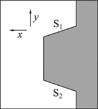
a:	b:
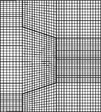
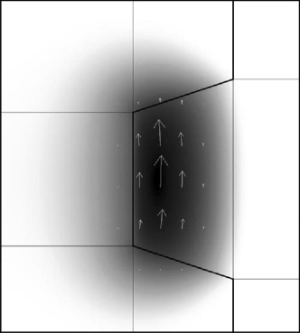
c:	d:

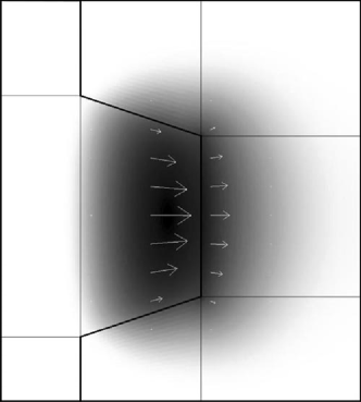
Figure 2: UWA’s sloping-shoulder cryogenic sapphire resonator: (a) medial cross-section through its geometry; the grey(white) shading corresponds to sapphire(vacuum); S₁ and S₂ indicate the sapphire piece’s upper and lower ‘shoulders’. (b) mesh of the resonator’s model structure generated by the FEM-based PDE-solver; for clarity, only every other meshing line is drawn [i.e. (b) displays the ‘half-mesh’]; within (c) and (d), the (logarithmic) grey scale reflects the absolute value of the vectorial magnetic H and electric E fields, respectively; white arrows indicate the magnitude and direction of each field’s medial component.

This axisymmetric resonator [42] comprises a piece of monocrystalline sapphire mounted (co-axially) within a cylindrical metal can –see Fig. 2(a); the crystal’s optical (or ‘c’) axis lies parallel to the resonator’s geometric axis. The piece’s sloping shoulders (S₁ and S₂ ibid.) make accurate simulation via mode-matching less straightforward. The resonator’s form, as encoded into the PDE-solver, is taken from figure 3 of ref. [9], with the piece’s outer diameter, the length of its outer axial sidewall, the axial extent of each sloping shoulder, and the radius of each of its two spindles equal to, at liquid-helium temperature (i.e. including cryogenic shrinkages –see section V) 49.97, 19.986, 4.996, and 19.988 mm, respectively. The sapphire crystal’s cryogenic permittivities were taken to be $\{\epsilon_{\perp},\epsilon_{\parallel}\}=\{9.2725,11.3486\}$, as given in ref. [20]. Since the sapphire piece and its surrounding metal can do not share a common transverse (‘equatorial’) mirror plane, the speeding up of the simulation through the imposition of a magnetic or electric wall on such a plane (so halving the 2D region to be analyzed) is precluded.

Fig. 2(b) displays the FEM-based PDE-solver’s meshing of the model resonator’s structure; in COMSOL’s vernacular, the mesh comprises 7296 base-mesh elements and 88587 degrees of freedom (‘DOF’). It took typically 75 seconds, to obtain the resonator’s lowest (in frequency) 16 modes, for a single, given azimuthal mode order $M$, at [with respect to Fig. 2(b)] full mesh density, on a standard, 2004-vintage personal computer (2.4 GHz, Intel Xeo CPU), without altering the PDE-solver’s default eigensolver settings. With the azimuthal mode order set at $M=14$, the model resonator’s WGE_14,0,0 mode was found to lie at 11.925 GHz, to be compared with 11.932 GHz found experimentally [9].

Wall loss: This mode’s characteristic length $\Lambda$, as evaluated with respect to the can wall’s enclosing surface, was determined to be $2.6\times 10^{4}$ m. Based on ref. [37], one estimates the surface resistance of copper at liquid-helium temperature to be $7\times 10^{-3}\;\Omega$ per square at 11.9 GHz, leading to a wall-loss $Q$ of $3.5\times 10^{11}$ for the WGE_14,0,0 mode.

Filling factor: Using equation 25, the electric filling factors for the WGE_14,0,0 mode were evaluated. These factors, presented in TABLE I above, are in good agreement with those labeled ‘FE’ in Table IV of ref. [9], that were obtained via a wholly independent FEM simulation of the same resonator.

TABLE I: Electric filling factors for the WGE_14,0,0 mode of UWA’s sloping-shoulders resonator

$F_{\rm{diel.}}^{\rm{dir.}}$	radial	azimuthal	axial
sapphire	0.80922	0.16494	$7.016\times 10^{-3}$
vacuum	0.01061	$8.0533\times 10^{-3}$	$1.6543\times 10^{-4}$

IV-B Toroidal silica optical resonator [Caltech]

a:

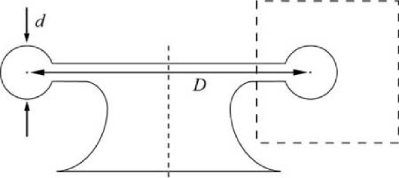
b:

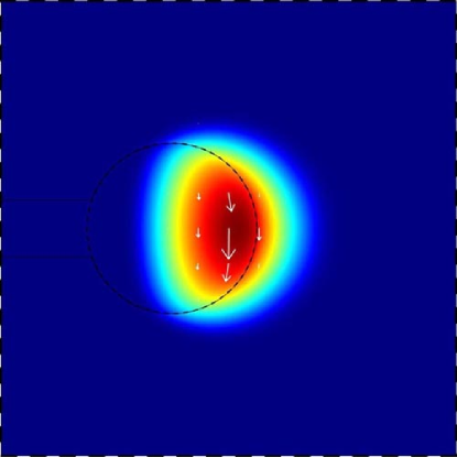
Figure 3: (a) Geometry (medial cross-section) and dimensions of a model toroidal silica microcavity resonator –after ref. [11]; the torus’ principal diameter $D=16$ $\mu$m and its minor diameter $d=3$ $\mu$m; the central vertical dashed line indicates the resonator’s axis of continuous rotational symmetry. (b) False-color surface plot of the (logarithmic) electric-field intensity $|\textbf{E}|^{2}$ over the dashed box appearing in (a) for this resonator’s TE_p=1,m=93 whispering-gallery mode; white arrows indicate the electric field’s magnitude and direction in the medial plane.

The resonator modeled here, based on ref. [11], comprises a silica toroid, supported above a substrate by an integral interior ‘web’; its geometry is shown in Fig. 3(a). The toroid’s principal and minor diameters are $\{D,d\}$ = $\{16,3\}$ $\mu$m, respectively. The silica dielectric is presumed to be wholly isotropic (i.e., no significant residual stress) with a relative permittivity of $\epsilon_{\rm{sil.}}=2.090$, corresponding to a refractive index of $n_{\rm{sil.}}=\sqrt{\epsilon_{\rm{sil.}}}=1.4457$ at the resonator’s operating wavelength (around 852 nm) and temperature. The FEM model’s pseudo-random triangular mesh covered an 8-by-8 $\mu$m square [shown in dashed outlined on the right of Fig. 3(a)], with an enhanced meshing density over the silica circle and its immediately surrounding free-space; in total, the mesh comprised 5990 (base-mesh) elements, with DOF $=36279$. Temporarily adopting Spillane et al’s terminology, the resonator’s fundamental TE-polarized 93rd-azimuthal-mode-order mode (where ‘TE’ here implies that the polarization of the mode’s electric field is predominantly aligned with the toroid’s principal axis –not transverse to it) was found to have a frequency of $3.532667\times 10^{14}$ Hz, corresponding to a free-space wavelength of $\lambda$ = 848.629 nm (thus close to 852 nm). Using equation 24, this mode’s volume was evaluated to be 34.587 $\mu$m³; if, instead, the definition stated in equation 5 of ref. [11] is used, the volume becomes 72.288 $\mu$m³ –i.e. a factor of $n_{\rm{sil.}}^{2}$ greater. These two values straddle the volume of $\sim$55 $\mu$m³, for the same dimensions of silica toroid and (TE) mode-polarization, as inferred by eye from figure 4 of ref. [11].

IV-C Conical microdisk optical resonator [Caltech]

The mode volume can be reduced by going to smaller resonators, which, unless the optical wavelength is commensurately reduced, implies lower azimuthal mode orders.

a:

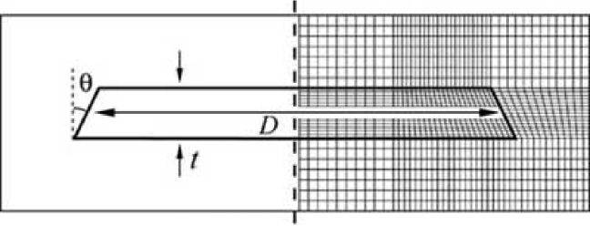
b:

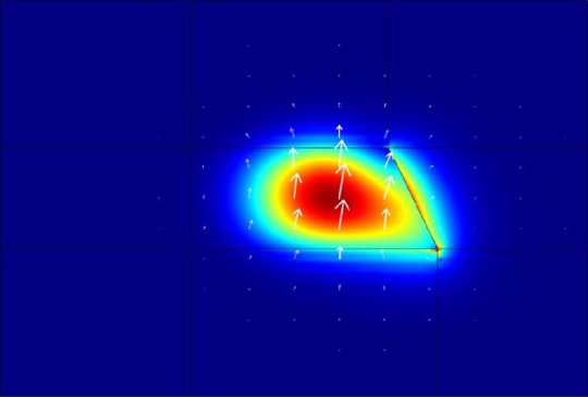
Figure 4: (a) Geometry (medial cross-section) and (half-)meshing of model GaAlAs microdisk resonator –after ref. [12]; the disk’s median diameter is $D$ = 2.12 $\mu$m and its thickness (axial height) $t$ = 255 nm; its conical external sidewall subtends an angle $\theta$ = 26^∘ to the disk’s (vertical) axis; for clarity, only every other line of the true (full) mesh is drawn. The modeled domain in the medial half-plane is a rectangle stretching from 0.02 to 1.5 $\mu$m in the radial direction and from -0.5 to +0.5 $\mu$m in the axial direction. (b) False-color surface plot of the (logarithmic) electric-field intensity $|\textbf{E}|^{2}$ for the resonator’s TE_p=1,m=11 mode at $\lambda$ = 1263.6 nm; again, white arrows indicate the electric field’s magnitude and direction in the medial plane.

The model ‘microdisk’ resonator analyzed here, as depicted in Fig. 4(a), duplicates the structure defined in figure 1(a) of Srinivasan et al [12]; the disk’s constituent dielectric (alternate layers of GaAs and GaAlAs) is approximated as a spatially uniform, isotropic dielectric, with a refractive index equal to $n$ = 3.36. The FEM-modeled domain comprised 4928 quadrilateral base-mesh elements, with DOF $=60003$. Adopting the same authors’ notation, the resonator’s TE_p=1,m=11 whispering-gallery mode, as shown in Fig. 4(b), was found at $2.372517\times 10^{14}$ Hz, equating to $\lambda$ = 1263.6 nm; for comparison, Srinivasan et al found an equivalent mode at 1265.41 nm [as depicted in their figure 1(b)]. It is pointed out here that the white electric-field arrows in Fig. 4(b) [and also, though to a lesser extent, in Fig. 3(b)] are not perfectly vertical –as the transverse approximation taken in references [9, 29] would assume them to be; the quasi-ness of the true mode’s transverse-electric polarization is thus revealed.

Mode volume: Using equation 24, but with the mode excited as a standing-wave (doubling the numerator while quadrupling the denominator), the mode volume is determined to be $0.1484\times\mu$m${}^{3}\simeq 2.79(\lambda/n)^{3}$, still in good agreement with Srinivasan et al’s $\sim\!2.8(\lambda/n)^{3}$.

Radiation loss: The TE_p=1,m=11 mode’s radiation loss was estimated by implementing both the upper- and lower-bounding estimators described in subsection III-E. Here, the microdisk and its mode were modeled over an approximate sphere, equating to a half-disk in 2D (medial plane). The half-disk’s diameter was 12 $\mu$m and different electromagnetic conditions were imposed on its semicircular boundary–see Fig. 5.

a:

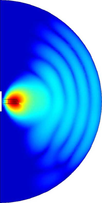
b:

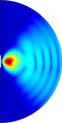
c:

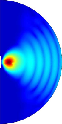
Figure 5: Radiation associated with the same [TE_p=1,m=11, $\lambda$ = 1263.6 nm] whispering-gallery mode as presented in Fig. 4 (all three maps use the same absolute false-color scale): (a) standing-wave (equal outward- and inward-going) radiation with the outer semicircular boundary set as a magnetic wall; (b) the same but now with the boundary set as an electric wall; (c) somewhat traveling (more outward- than inward-going) radiation with the boundary’s impedance set to that of an outward-going plane-wave in free space (and with the normal magnetic field constrained to vanish). That (c)’s radiation field is somewhat dimmer than (b)’s is consistent with the two different estimates of the resonator’s radiative $Q$ corresponding to (b) and (c) [see text].

With an electric-wall condition (i.e. equations 2 and 3 or, equivalently, 17 and {18, 20}) imposed on the half-disk’s entire boundary [as per Fig. 5(b)], the right-hand of equation 28 was evaluated. And, with the $\textbf{E}\boldsymbol{\times}\textbf{n}=0$ condition (viz. equation 3) on the boundary’s semicircle replaced by the outward-going-plane-wave(-in-free-space) impedance-matching condition (viz. equation 29 with $\theta_{\rm{mix}}=\pi/4$), while the $\textbf{H}\cdot\textbf{n}=0$ condition (equation 2) is maintained, the right-hand side of equation 30 was evaluated for the radiation pattern displayed in Fig. 5(c). For a pseudo-random triangulation mesh comprising 4104 elements, with DOF $=24927$, the PDE solver took, on the author’s office computer, 6.55 and 13.05 seconds, corresponding to Figs. 5(b) and (c), respectively, to calculate 10 eigenmodes around $2.373\times 10^{14}$ Hz, of which the TE_p=1,m=11 mode was one. Together, the resultant estimate on the TE_p=1,m=11 mode’s radiative-loss quality factor is $(1.31<Q_{\rm{rad.}}<3.82)\times 10^{7}$, to be compared with the estimate of $9.8\times 10^{6}$ (at 1265 nm) reported in table 1 of ref. [12].

IV-D Distributed-Bragg-reflector microwave resonator

The method’s ability to simulate axisymmetric resonators of arbitrary cross-sectional complexity is demonstrated here by simulating the 10-GHz TE₀₁ mode of a distributed-Bragg-reflector (DBR) resonator as analyzed by Flory and Taber (F&T) [43] through mode matching.

a:

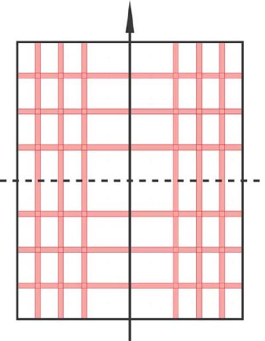
b:

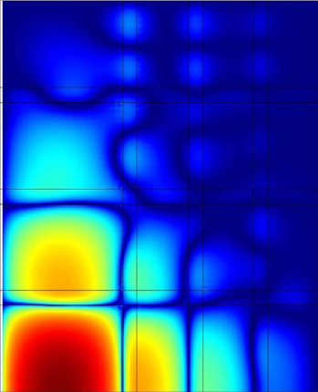
Figure 6: (a) Geometry (medial cross-section) of a 3rd-order distributed-Bragg-reflector resonator within a cylindrical metallic can (hence electric interior walls –represented by a solid black rectangle); as per ref. [43], the can’s interior diameter is 10.98 cm and its interior height is 13.53 cm; the horizontal and vertical grey (or pink –in color reproduction) stripes denote cylindrical plates and barrels of sapphire; white rectangles correspond to right cylinders/annuli of free-space; the vertical arrow indicates the resonator’s axis of rotational symmetry, with which the sapphire crystal’s c-axis is aligned; a magnetic wall is imposed over the resonator’s equatorial plane of mirror symmetry (dashed horizontal line; cf. M1 in Fig. 1). (b) False-color plot of the (logarithmic) electric-field intensity $|\textbf{E}|^{2}$ over the top-right medial quadrant of the rotationally invariant ($M=0$) TE₀₁ mode; note how the mode is strongly localized within the resonator’s central cylinder of free-space

The resonator’s model geometry was generated through an auxiliary script written in MATLAB. Its corresponding mesh comprised 5476 base-mesh elements, with 66603 degrees of freedom (DOF), with 8 edge vertices for each $\sim\!\!\lambda/4$ layer of sapphire. Based on ref. [44]’s quartic fitting polynomials, the sapphire crystal’s dielectric permittivities, at a temperature $T=300$ K, were set to $\epsilon_{\perp}=9.394$ (consistent with ref. [43]) and $\epsilon_{\parallel}=11.593$. The TE₀₁ mode shown in Fig. 6(b) was found to lie at 10.00183 GHz, in good agreement with F&T’s ‘precisely 10.00 GHz’. Using equation 25, the mode’s electric filling factor for the resonator’s sapphire parts was 0.1270, which, assuming an (isotropic) loss tangent of $5.9\times 10^{-6}$ as per F&T, corresponds to a dielectric-loss $Q$ factor of 1.334 million. Through equations 26 and 27, and assuming a surface resistance of 0.026 $\Omega$ per square as per F&T, the wall-loss $Q$ factor was determined to be 29.736 million, leading to a composite $Q$ (for dielectric and wall losses operating in tandem) of 1.278 million. These three $Q$ values are consistent with F&T’s stated (composite) $Q$ of ‘1.3 million, and limited entirely by dielectric losses’.

a:

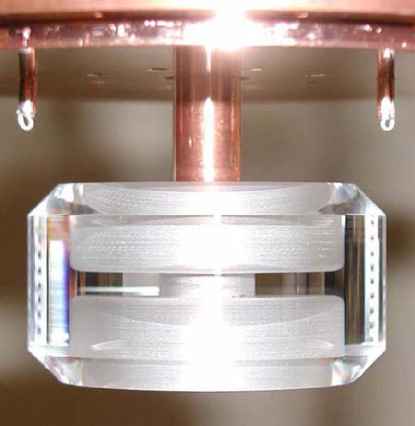
b:

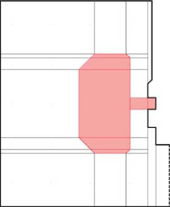
c:

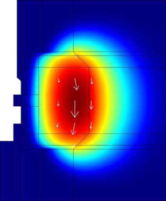
Figure 7: (a) Close-up of NPL’s cryo-sapphire resonator, with the main body of its outer copper can removed. The resonator’s chamfered HEMEX sapphire ring has an outer diameter of $\sim$46.0 mm and an axial height of $\sim$25.1 mm. The ring’s integral interior ‘web’, 3mm thick, lies parallel to, and is centered (axially) on, the ring’s equatorial plane, and is supported through a central copper post. Optical refraction at the ring’s outer surface falsely exaggerates its internal diameter. Above the ring are two loop probes for coupling electromagnetically to the resonator’s operational whispering-gallery mode. (b) geometry of the resonator in medial cross-section; pink/grey indicates sapphire, white free space; bounding these dielectric domains, and shown as solid black lines, are copper surfaces belonging to the resonator’s can and web-supporting post [the dashed vertical line (lower right) runs along the resonator’s cylindrical axis ($r=0$)]. (c) false-color map (logarithmic scale) of $|\textbf{H}|^{2}$ for the resonator’s 11th-azimuthal-mode-order fundamental quasi-transverse-magnetic (N1₁₁ in ref. [7]’s notation) whispering-gallery mode at 9.146177 GHz (simulated), as detailed on the 6th row of TABLE II. The white arrows indicate the magnitude and direction of this mode’s electric field strength (E) in the medial plane.

V Determination of the permittivities of cryogenic sapphire

TABLE II: NPL’s cryogenic sapphire resonator: simulated and experimental WG modes compared

Simulated	Simul.	Simul.	Mode	Experi-	Exper.	Exper.	Exper.
minus	perp.	para.	ID	mental	width	turn-	Kram.
experim.	filing	filling		freq.		over	split.
frequency	factor	factor				temp.
$[$MHz$]$				$[$GHz$]$	$[$Hz$]$	$[$K$]$	$[$Hz$]$
-0.451	0.860	0.090	S26	6.954664	285		780
-0.945	0.930	0.028	S27	7.696176	82.5	$<4.2$	158
0.881	0.453	0.517	S46	8.430800
-1.538	0.951	0.014	S28	8.449908	44.5	$<4.2$	418
-0.412	0.674	0.299	N28	9.037458		$4.8$
-2.208	0.071	0.917	N111	9.148385	9	$5.0$	57
-1.916	0.960	0.009	S29	9.204722	15.5	$<4.2$	88
0.498	0.251	0.733	S110	9.267650	12	$5.2$	180
1.055	0.287	0.685	N48	9.421207	80	$5.0$
-0.177	0.437	0.543	S38	9.800335	84	$4.8$	1850
0.358	0.223	0.763	S111	9.901866	10	$5.0$	160
-2.269	0.965	0.007	S210	9.957880	24	$<4.2$
1.32	0.730	0.246	S48	10.27242	153	$5.0$
0.19	0.200	0.787	S112	10.53863	9.5	$4.9$	24
0.00	0.181	0.808	S113	11.17728	24.5	$4.9$	42
4.13	0.972	0.006	S212	11.44918	10	$5.2$

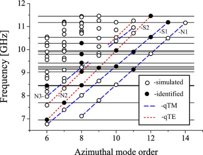
Figure 8: Plot used to aid the identification of experimental with simulated WG modes. Solid horizontal lines (16 in total) indicate the center frequencies of the former. Solid circles indicate the identification of a simulated mode with an experimental one (the difference in their frequencies corresponds to much less than a circle’s radius in all cases); hollow circles indicate simulated modes that were not identified with any experimentally measured one. Quasi-transverse-magnetic (q-TM) and quasi-transverse-electric (q-TE) WG modes of the same family are joined by (blue-)dashed and (red-)dotted lines respectively; a few of the lowest-lying mode families are labeled using standard notation [7].

The method is here applied to determine the two dielectric constants of monocrystalline sapphire (HEMEX grade [45]) at 4.2 K from a set of experimental data, listed in the four right-most columns of TABLE II, and corresponding to the resonator whose innards are shown in Fig. 7(a). Allowance was made for the shrinkages of the resonator’s constituent materials from room to liquid-helium temperature and the values of sapphire’s two dielectric constants ($\epsilon_{\perp}$ and $\epsilon_{\parallel}$) were initially set equal to those specified in ref. [20]. Fig. 7(b)’s geometry was meshed with quadrilaterals over the medial half-plane, with 8944 elements in its base mesh, and with DOF $=108555$. For a given azimuthal mode order $M$, calculating the lowest 16 eigenmodes took around 3 minutes on the author’s office PC (as previously specified). With Fig. 8 as a guide, each of the 16 experimental resonances was identified to a particular simulated WG mode, as specified in the 4th column of TABLE II, lying near to it in frequency; these identifications were influenced by requiring that the measured attributes (e.g. the FWHM linewidths) of the experimental resonances belonging –as per their identifications– to the same ‘family’ of WG modes (e.g. S1, or N2) varied smoothly with $M$. Filling factors were then calculated to quantify the differential change in the frequency of each identified mode with respect to $\epsilon_{\perp}$ and $\epsilon_{\parallel}$. The two dielectric constants were then adjusted to minimize the $\chi^{2}$ variance of the residual (simulated-minus-measured) frequency differences. The resultant best-fit values, to which the simulated data occupying the three left-most columns in TABLE II correspond, were:

$$\epsilon_{\perp} = 9.285\,\,(\pm 0.010);$$ (31)

$$\epsilon_{\parallel} = 11.366\,\,(\pm 0.010).$$ (32)

The nominal error assigned to each reflects uncertainties in the identifications of certain experimental resonances, each lying almost equally close (in both frequency and other attributes) to two or more different simulated WG modes. Errors resulting from a finite meshing density [33], or those from the finite dimensional/geometric tolerances to which the resonator’s shape was known, were estimated to be small in comparison.

Mark Oxborrow was born near Salisbury, England, in 1967. He received a B.A. in physics from the University of Oxford in 1988, and a Ph.D. in theoretical condensed-matter physics from Cornell University in 1993; his thesis topic concerned random-tiling models of quasicrystals. During subsequent postdoctoral appointments at both the Niels Bohr Institute in Copenhagen and then back at Oxford, he investigated acoustic analogues of quantum wave-chaos. In 1998, he joined the UK’s National Physical Laboratory; his eclectic, project-based research work there to date has included the design and construction of ultra-frequency-stable microwave and optical oscillators, the development of single-photon sources, and the applications of carbon nanotubes to metrology.

References

- [1] K. S. Kunz, The finite difference time domain method for electromagnetics. CRC Press, 1993.
- [2] S. V. Boriskina, T. M. Benson, P. Sewell, and A. I. Nosich, “Highly efficient design of specially engineered whispering-gallery-mode laser resonators,” Optical and Quantum Electronics, vol. 35, pp. 545–559, 2003, see http://www.nottingham.ac.uk/ggiemr/Project/-boriskina2.htm.
- [3] J. Ctyroky, L. Prkna, and M. Hubalek, “Rigorous vectorial modelling of microresonators,” in Proc. 2004 6th Internat. Conf. on Transparent Optical Networks, 4-8 July 2004, vol. 2, 2004, pp. 281–286.
- [4] O. C. Zienkiewicz and R. L. Taylor, The finite element method, 5th ed. Butterworth Heinemann, 2000, vol. 1: ‘The Basis’.
- [5] M. M. Taheri and D. Mirshekar-Syahkal, “Accurate determination of modes in dielectric-loaded cylindrical cavities using a one-dimensional finite element method,” IEEE Trans. Microwave Theory Tech., vol. 37, no. 10, pp. 1536–1541, 1989.
- [6] J. U. Nöckel and A. D. Stone, “Ray and wave chaos in asymmetric resonator optical cavities,” Nature, vol. 385, pp. 45–47, 1997.
- [7] M. E. Tobar, J. G. Hartnett, E. N. Ivanov, P. Blondy, and D. Cros, “Whispering gallery method of measuring complex permittivity in highly anisotropic materials: discovery of a new type of mode in anisotropic dielectric resonators,” IEEE Trans. Instrum. and Meas., vol. 50, no. 2, pp. 522–525, 2001.
- [8] M. Sumetsky, “Whispering-gallery-bottle microcavities: the three-dimensional etalon,” Opt. Lett., vol. 29, pp. 8–10, 2004.
- [9] P. Wolf, M. E. Tobar, S. Bize, A. Clairon, A. Luiten, and G. Santarelli, “Whispering gallery resonators and tests of Lorentz invariance,” General Relativity and Gravitation, vol. 36, no. 10, pp. 2351 – 2372, 2004, and are stated for sapphire at 4 K; preprint version: arXiv:gr-qc/0401017 v1.
- [10] H. Rokhsari, T. Kippenberg, T. Carmon, and K. J. Vahala, “Radiation-pressure-driven micro-mechanical oscillator,” Opt. Express, vol. 13, pp. 5293–5301, 2005.
- [11] S. M. Spillane, T. J. Kippenberg, K. J. Vahala, K. W. Goh, E. Wilcut, and H. J. Kimble, “Ultrahigh-Q toroidal microresonators for cavity quantum electrodynamics,” Phys. Rev. A., vol. 71, p. 013817, 2005.
- [12] K. Srinivasan, M. Borselli, O. Painter, A. Stintz, and S. Krishna, “Cavity Q, mode volume, and lasing threshold in small diameter AlGaAs microdisks with embedded quantum dots,” Opt. Express, vol. 14, pp. 1094–1105, 2006.
- [13] “MAFIA,” CST GmbH, Bad Nauheimer Str. 19, D-64289 Darmstadt Germany. [Online]. Available: http://www.cst.de/Content/-Products/MAFIA/Overview.aspx.
- [14] R. Basu, T. Schnipper, and J. Mygind, “10 GHz oscillator with ultra low phase noise,” in Proc. The Jubilee 8th International Workshop ‘From Andreev Reflection to the International Space Station’, Björkliden, Kiruna, Sweden, March 20-27, 2004, 2004. [Online]. Available: http://fy.chalmers.se/f4agro/BJ2004/FILES/Bjorkliden_art.pdf.
- [15] I. G. Wilson, C. W. Schramm, and J. P. Kinzer, “High Q resonant cavities for microwave testing,” Bell Syst. Tech. J., vol. 25, pp. 408–34, 1946.
- [16] S. Ramo, J. R. Whinnery, and T. van Duzer, Fields and Waves in Communications Electronics, 2nd ed. John Wiley & Sons, 1984.
- [17] U. S. Inan and A. S. Inan, Electromagnetic Waves. Prentice Hall, 2000, particularly subsection 5.3.2 (pp. 391-400).
- [18] M. E. Tobar, “Resonant frequencies of higher order modes of cylindrical anisotropic dielectric resonators,” IEEE Trans. Microwave Theory Tech., vol. 39, no. 12, pp. 2077–82, 1991.
- [19] J. G. Harnett and M. E. Tobar, “Determination of whispering gallery modes in a uniaxial cylindrical sapphire crystal,” 2004, Mathematica code/notebook, private correspondence.
- [20] J. Krupka, K. Derzakowski, A. Abramowicz, M. E. Tobar, and R. G. Geyer, “Use of whispering-gallery modes for complex permittivity determinations of ultra-low-loss dielectric materials,” IEEE Trans. Microwave Theory Tech., vol. 47, no. 6, pp. 752–759, 1999, this paper provides and for sapphire at 4.2 K.
- [21] J. Krupka, D. Cros, M. Aubourg, and P. Guillon, “Study of whispering gallery modes in anisotropic single-crystal dielectric resonators,” IEEE Trans. Microwave Theory Tech., vol. 42, no. 1, pp. 56–61, 1994.
- [22] J. Krupka, D. Cros, A. Luiten, and M. Tobar, “Design of very high Q sapphire resonators,” Electronics Letters, vol. 32, no. 7, pp. 670–671, 1996.
- [23] J. A. Monsoriu, M. V. Andrés, E. Silvestre, A. Ferrando, and B. Gimeno, “Analysis of dielectric-loaded cavities using an orthonormal-basis method,” IEEE Trans. Microwave Theory Tech., vol. 50, no. 11, pp. 2545–2552, 2002.
- [24] N. M. Alford, J. Breeze, S. J. Penn, and M. Poole, “Layered Al2O3-TiO2 composite dielectric resonators with tuneable temperature coefficient for microwave applications,” IEE Proc. Science, Measurement and Technology, vol. 47, pp. 269–273, 2000.
- [25] J. P. Wolf, The scaled boundary finite element method. Wiley, 2003.
- [26] B. M. A. Rahman, F. A. Fernandez, and J. B. Davies, “Review of finite element methods for microwave and optical waveguides,” Proc. IEEE, vol. 79, pp. 1442–1448, 1991.
- [27] “COMSOL Multiphysics,” COMSOL, Ab., Tegnérgatan 23, SE-111 40 Stockholm, Sweden. [Online]. Available: http://www.comsol.com/, the work described in this paper used 3.2(.0.224).
- [28] “ANSYS Multiphysics,” ANSYS, Inc., Southpointe, 275 Technology Drive, Canonsburg, PA 15317, USA. [Online]. Available: http://www.ansys.com/.
- [29] T. J. A. Kippenberg, “Nonlinear optics in ultra-high-Q whispering-gallery optical microcavities,” Ph.D. dissertation, Caltech, 2004, particularly Appendix B. [Online]. Available: http://www.mpq.mpg.de/-∼tkippenb/TJKippenbergThesis.pdf.
- [30] A. Auborg and P. Guillon, “A mixed finite element formulation for microwave device problems. application to MIS structure,” J. Electromagn. Wave Appl., vol. 5, pp. 371–386, 1991.
- [31] J.-F. Lee, G. M. Wilkins, and R. Mittra, “Finite-element analysis of axisymmetric cavity resonator using a hybrid edge element technique,” IEEE Trans. Microwave Theory Tech., vol. 41, no. 11, pp. 1981–7, 1993.
- [32] R. A. Osegueda, J. H. Pierluissi, L. M. Gil, A. Revilla, G. J. Villava, G. J. Dick, D. G. Santiago, and R. T. Wang, “Azimuthally-dependent finite element solution to the cylindrical resonator,” Univ. Texas, El Paso and JPL, Caltech, Tech. Rep. [Online]. Available: http://trs-new.jpl.nasa.gov/dspace/bitstream/2014/32335/1/94-0066.pdf or http://hdl.handle.net/2014/32335.
- [33] D. G. Santiago, R. T. Wang, G. J. Dick, R. A. Osegueda, J. H. Pierluissi, L. M. Gil, A. Revilla, and G. J. Villalva, “Experimental test and application of a 2-D finite element calculation for whispering gallery sapphire resonators,” in IEEE 48th International Frequency Control Symposium, 1994, Boston, MA, USA, pp. 482–485. [Online]. Available: http://trs-new.jpl.nasa.gov/dspace/bitstream/2014/33066/1/94-1000.pdf or http://hdl.handle.net/2014/33066.
- [34] B. I. Bleaney and B. Bleaney, Electricity and magnetism, 3rd ed. Oxford University Press, 1976.
- [35] F. N. H. Robinson, Macroscopic Electromagnetism, ser. International Series of Monographs in Natural Philosophy, D. t. Haar, Ed. Pergamon Press, 1973, vol. 57.
- [36] F. Pobell, Matter and methods at low temperatures. Springer, 1992.
- [37] R. Fletcher and J. Cook, “Measurement of surface impedance versus temperature using a generalized sapphire resonator technique,” Rev. Sci. Instr., vol. 65, pp. 2658–2666, 1994.
- [38] P.-Y. Bourgeois, F. Lardet-Vieudrin, Y. Kersale, N. Bazin, M. Chaubet, and V. Giordano, “Ultra-low drift microwave cryogenic oscillator,” Electronics letters, vol. 40, p. 605, 2004.
- [39] S. A. Schelkunoff, “Some equivalence theorems of electromagnetics and their application to radiation problems,” Bell Syst. Tech. J., vol. 15, pp. 92+, 1936.
- [40] C. A. Balanis, Antenna Theory. Wiley, 1997, particularly chapter 12.
- [41] S. A. Schelkunoff, “On diffraction and radiation of electromagnetic waves,” Physical Review, vol. 56, no. 4, pp. 308 LP – 316, 1939.
- [42] A. N. Luiten, A. G. Mann, N. J. McDonald, and D. G. Blair, “Latest results of the U.W.A. cryogenic sapphire oscillator,” in Proc. of IEEE International 49th Frequency Control Symposium, San Francisco, CA, USA, 1995, pp. 433–437.
- [43] C. A. Flory and R. C. Taber, “High performance distributed bragg reflector microwave resonator,” IEEE Trans. Ultrason. Ferroelect. Freq. Contr., vol. 44, no. 2, pp. 486–495, 1997, specifically, the mode corresponding to figures 1, 2 and 7, and the last three paragraphs of section IV therein.
- [44] ——, “Microwave oscillators incorporating cryogenic sapphire dielectric resonators,” in IEEE International Frequency Control Symposium 1993, 1993, pp. 763–773.
- [45] “HEM Sapphire,” Crystal Systems, Inc., Salem, MA, USA. [Online]. Available: http://www.crystalsystems.com/sapprop.html.
- [46] G. K. White and R. B. Roberts, “Thermal expansion of reference materials: tungsten and -Al2O3,” High Temperatures - High Pressures, vol. 15, pp. 321–328, 1983.
- [47] G. K. White, “Reference materials for thermal expansion: certified or not?”, Thermochimica Acta, vol. 218, pp. 83–99, 1993.
- [48] ——, Experimental techniques in low-temperature physics, 3rd ed. Clarendon Press, Oxford, 1979.