Coherent control in a decoherence-free subspace of a collective multi-level system

Abstract

Decoherence-free subspaces (DFS) in systems of dipole-dipole interacting multi-level atoms are investigated theoretically. It is shown that the collective state space of two dipole-dipole interacting four-level atoms contains a four-dimensional DFS. We describe a method that allows to populate the antisymmetric states of the DFS by means of a laser field, without the need of a field gradient between the two atoms. We identify these antisymmetric states as long-lived entangled states. Further, we show that any single-qubit operation between two states of the DFS can be induced by means of a microwave field. Typical operation times of these qubit rotations can be significantly shorter than for a nuclear spin system.

I INTRODUCTION

The fields of quantum computation and quantum information processing have attracted a lot of attention due to their promising applications such as the speedup of classical computations Chuang et al. (1995); Ekert and Jozsa (1996); Nielsen and Chuang (2000). Although the physical implementation of basic quantum information processors has been achieved recently Monroe (2002), the realization of powerful and useable devices is still a challenging and as yet unresolved problem. A major difficulty arises from the interaction of a quantum system with its environment, which leads to decoherence DiVincenzo (1995); Unruh (1995). One possible solution to this problem is provided by the concept of decoherence-free subspaces (DFS) Zanardi and Rasetti (1997); Lidar et al. (1998); lid ; Kempe et al. (2001); Knill et al. (2000); Shabani and Lidar (2005). Under certain conditions, a subspace of a physical system is decoupled from its environment such that the dynamics within this subspace is purely unitary. Experimental realizations of DFS have been achieved with photons Kwiat et al. (2000); Zhang et al. (2006); Altepeter et al. (2004); Mohseni et al. (2003) and in nuclear spin systems Viola et al. (2001); Wei et al. (2005); Ollerenshaw et al. (2003). A decoherence-free quantum memory for one qubit has been realized experimentally with two trapped ions Kielpinski et al. (2001); Langer et al. (2005).

The physical implementation of most quantum computation and quantum information schemes involves the generation of entanglement and the realization of quantum gates. It has been shown that dipole-dipole interacting systems are both a resource for entanglement and suitable candidates for the implementation of gate operations between two qubits Bargatin et al. (2000); Ficek and Tanaś (2002); Lukin and Hemmer (2000); Beige et al. (2000); Brennen et al. (1999); Jaksch et al. (2000); Barenco et al. (1995). The creation of entanglement in collective two-atom systems is discussed in Bargatin et al. (2000); Ficek and Tanaś (2002). Several schemes employ the dipole-dipole induced energy shifts of collective states to realize quantum gates, for example, in systems of two atoms Lukin and Hemmer (2000); Beige et al. (2000); Brennen et al. (1999); Jaksch et al. (2000) or quantum dots Barenco et al. (1995). In order to ensure that the induced dynamics is fast as compared to decoherence processes, the dipole-dipole interaction must be strong, and thus the distance between the particles must be small. On the other hand, it is well known that a system of particles which are closer together than the relevant transition wavelength displays collective states which are immune against spontaneous emission aga ; Ficek and Swain (2005); Mandel and Wolf (1995); Ficek and Tanaś (2002); Dicke (1954). The space spanned by these subradiant states is an example for a DFS, and hence the question arises whether qubits and gate operations enabled by the coherent part of the dipole-dipole interaction can be embedded into this DFS. In the simple model of a pair of interacting two-level systems, there exists only a single subradiant state. Larger DFS which are suitable for the storage and processing of quantum information can be found, e.g., in systems of many two-level systems Zanardi (1997); Duan and Guo (1998).

Here, we pursue a different approach and consider a pair of dipole-dipole interacting multi-level atoms [see Fig. 1]. The level scheme of each of the atoms is modeled by a $S_{0}\leftrightarrow P_{1}$ transition that can be found, e.g., in ⁴⁰Ca atoms. The excited state multiplet $P_{1}$ consists of three Zeeman sublevels, and the ground state is a $S_{0}$ singlet state. We consider arbitrary geometrical alignments of the atoms, i.e. the length and orientation of the vector $\boldsymbol{R}$ connecting the atoms can be freely adjusted. In this case, all Zeeman sublevels of the atomic multiplets have to be taken into account kif . Experimental studies of such systems have become feasible recently DeVoe and Brewer (1996); Hettich et al. (2002); Eschner et al. (2001).

As our main results, we demonstrate that the state space of the two atoms contains a 4-dimensional DFS if the interatomic distance $R$ approaches zero. A careful analysis of both the coherent and the incoherent dynamics reveals that the antisymmetric states of the DFS can be populated with a laser field, and that coherent dynamics can be induced within the DFS via an external static magnetic or a radio-frequency field. Finally, it is shown that the system can be prepared in long-lived entangled states.

More specifically, all features of the collective two-atom system will be derived from the master equation for the two atoms which we discuss in Sec. II. To set the stage, we prove the existence of the 4-dimensional DFS in the case of small interatomic distance $R$ in Sec. III.

Subsequent sections of this paper address the question whether this DFS can be employed to store and process quantum information. In a first step, we provide a detailed analysis of the coherent and incoherent system dynamics (Sec. IV). The eigenstates and energies in the case where the Zeeman splitting $\delta$ of the excited states vanishes are presented in Sec. IV.1. In Sec. IV.2, we calculate the decay rates of the collective two-atom states which are formed by the coherent part of the dipole-dipole interaction. It is shown that spontaneous emission in the DFS is strongly suppressed if the distance between the atoms is small as compared to the wavelength of the $S_{0}\leftrightarrow P_{1}$ transition. The full energy spectrum in the presence of a magnetic field is investigated in Sec. IV.3.

The DFS is comprised of the collective ground state and three antisymmetric collective states. In Sec. V, we show that the antisymmetric states can be populated selectively by means of an external laser field. The probability to find the system in a (pure) antisymmetric state is 1/4 in steady state. In particular, the described method does not require a field gradient between the position of the two atoms.

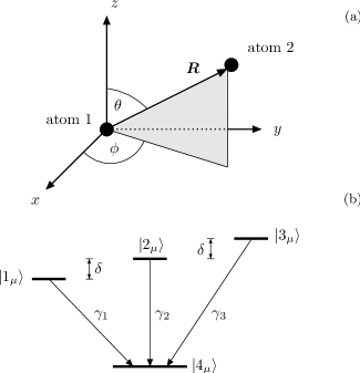
Figure 1: (a) The system under consideration is comprised of two atoms that are located at $\boldsymbol{r}_{1}$ and $\boldsymbol{r}_{2}$, respectively. The relative position $\boldsymbol{R}=\boldsymbol{r}_{2}-\boldsymbol{r}_{1}$ of atom 2 with respect to atom 1 is expressed in terms of spherical coordinates. (b) Internal level structure of atom $\mu\in\{1,2\}$. The ground state of each of the atoms is a $S_{0}$ state, and the three excited levels are Zeeman sublevels of a $P_{1}$ triplet. The states $|1_{\mu}\rangle$, $|2_{\mu}\rangle$ and $|3_{\mu}\rangle$ correspond to the magnetic quantum numbers $m_{j}=-1,\,0$ and 1, respectively. The frequency splitting of the upper levels is denoted by $\delta=\omega_{3}-\omega_{2}=\omega_{2}-\omega_{1}$, where $\hbar\omega_{i}$ is the energy of state $|i_{\mu}\rangle$.

We then address coherent control within the DFS, and demonstrate that the coherent time evolution of two states in the DFS can be controlled via the Zeeman splitting $\delta$ of the excited states and therefore by means of an external magnetic field (Sec. VI). Both static magnetic fields and radio-frequency (RF) fields are considered. The time evolution of the two states is visualized in the Bloch sphere picture. While a static magnetic field can only induce a limited dynamics, any single-qubit operation can be performed by an RF field.

In Sec. VII, we determine the degree of entanglement of the symmetric and antisymmetric collective states which are formed by the coherent part of the dipole-dipole interaction. We employ the concurrence as a measure of entanglement and show that the symmetric and antisymmetric states are entangled. The degree of entanglement of the collective states is the same as in the case of two two-level atoms. But in contrast to a pair of two-level atoms, the symmetric and antisymmetric states of our system are not maximally entangled.

A brief summary and discussion of our results is provided in Sec. VIII.

II EQUATION OF MOTION

In the absence of laser fields, the system Hamiltonian is given by

$$H=H_{A}+H_{F}+H_{\text{vac}}\,,$$ (1)

where

$$H_{A} = \hbar\sum\limits_{i=1}^{3}\sum\limits_{\mu=1}^{2}\omega_{i}\,S_{i\,+}^{(\mu)}S_{i\,-}^{(\mu)}\,,$$

$$H_{F} = \sum\limits_{\boldsymbol{k}s}\hbar\omega_{k}a_{\boldsymbol{k}s}^{\dagger}a_{\boldsymbol{k}s}\,,$$

$$H_{\text{vac}} = -\boldsymbol{\hat{d}}^{(1)}\cdot\boldsymbol{\hat{E}}(\boldsymbol{r}_{1})-\boldsymbol{\hat{d}}^{(2)}\cdot\boldsymbol{\hat{E}}(\boldsymbol{r}_{2})\,.$$ (2)

In these equations, $H_{A}$ describes the free evolution of the two identical atoms, $\hbar\omega_{i}$ is the energy of state $|i_{\mu}\rangle$ and we choose $\hbar\omega_{4}=0$. The raising and lowering operators on the $|4_{\mu}\rangle\leftrightarrow|i_{\mu}\rangle$ transition of atom $\mu$ are ($i\in\{1,2,3\}$)

$$S_{i\,+}^{(\mu)}=|i_{\mu}\rangle\langle 4_{\mu}|\quad\text{and}\quad S_{i\,-}^{(\mu)}=|4_{\mu}\rangle\langle i_{\mu}|\,.$$ (3)

$H_{F}$ is the Hamiltonian of the unperturbed vacuum field and $H_{\text{vac}}$ describes the interaction of the atom with the vacuum modes in dipole approximation. The electric field operator $\boldsymbol{\hat{E}}$ is defined as

$$\boldsymbol{\hat{E}}(\boldsymbol{r})=i\sum\limits_{\boldsymbol{k}s}\sqrt{\frac{\hbar\omega_{k}}{2\varepsilon_{0}V}}\boldsymbol{\epsilon}_{\boldsymbol{k}s}e^{i\boldsymbol{k}\cdot\boldsymbol{r}}a_{\boldsymbol{k}s}+\text{H.c.}\,,$$ (4)

where $a_{\boldsymbol{k}s}$ ($a_{\boldsymbol{k}s}^{\dagger}$) are the annihilation (creation) operators that correspond to a field mode with wave vector $\boldsymbol{k}$, polarization $\boldsymbol{\epsilon}_{\boldsymbol{k}s}$ and frequency $\omega_{k}$, and $V$ denotes the quantization volume. We determine the electric-dipole moment operator of atom $\mu$ via the Wigner-Eckart theorem Sakurai (1994) and arrive at

$$\boldsymbol{\hat{d}}^{(\mu)}=\sum\limits_{i=1}^{3}\big{[}\boldsymbol{d}_{i}S_{i\,+}^{(\mu)}+\text{H.c.}\big{]}\,,$$ (5)

where the dipole moments $\boldsymbol{d}_{i}=\langle i|\boldsymbol{\hat{d}}|4\rangle$ are given by

$$\begin{array}[]{rlrl}\boldsymbol{d}_{1}=&\mathcal{D}\,\boldsymbol{\epsilon}^{(+)}\,,&\boldsymbol{d}_{2}=&\mathcal{D}\,\boldsymbol{e}_{z}\,,\\[8.5359pt] \boldsymbol{d}_{3}=&-\mathcal{D}\,\boldsymbol{\epsilon}^{(-)}\,;&\boldsymbol{\epsilon}^{(\pm)}=&\frac{1}{\sqrt{2}}(\boldsymbol{e}_{x}\pm i\boldsymbol{e}_{y})\,,\end{array}$$ (6)

and $\mathcal{D}$ is the reduced dipole matrix element. Note that the dipole moments $\boldsymbol{d}_{i}$ do not depend on the index $\mu$ since we assumed that the atoms are identical.

With the total Hamiltonian $H$ in Eq. (1) we derive a master equation for the reduced atomic density operator $\varrho$. An involved calculation that employs the Born-Markov approximation yields kif ; Evers et al. (2006); Agarwal and Patnaik (2001); aga

$$\partial_{t}\varrho=-\frac{i}{\hbar}[H_{A},\varrho]-\frac{i}{\hbar}[H_{\Omega},\varrho]+\mathcal{L}_{\gamma}\varrho\,.$$ (7)

The coherent evolution of the atomic states is determined by $H_{A}+H_{\Omega}$, where $H_{A}$ is defined in Eq. (2). The Hamiltonian $H_{\Omega}$ arises from the vacuum-mediated dipole-dipole interaction between the two atoms and is given by

$$H_{\Omega} = -\hbar\sum\limits_{i=1}^{3}\left\{\Omega_{ii}S_{i\,+}^{(2)}S_{i\,-}^{(1)}\,+\,\text{H.c.}\right\}$$ (8)

$$-\hbar\left\{\Omega_{21}\left(S_{2\,+}^{(2)}S_{1\,-}^{(1)}+S_{2\,+}^{(1)}S_{1\,-}^{(2)}\right)\,+\,\text{H.c.}\right\}$$

$$-\hbar\left\{\Omega_{31}\left(S_{3\,+}^{(2)}S_{1\,-}^{(1)}+S_{3\,+}^{(1)}S_{1\,-}^{(2)}\right)\,+\,\text{H.c.}\right\}$$

$$-\hbar\left\{\Omega_{32}\left(S_{3\,+}^{(2)}S_{2\,-}^{(1)}+S_{3\,+}^{(1)}S_{2\,-}^{(2)}\right)\,+\,\text{H.c.}\right\}\,.$$

The coefficients $\Omega_{ij}$ cause an energy shift of the collective atomic levels (see Sec. IV) and are defined as kif ; Evers et al. (2006); Agarwal and Patnaik (2001)

$$\Omega_{ij}=\frac{1}{\hbar}\left[\boldsymbol{d}_{i}^{\text{T}}\;\text{Re}(\overset{\leftrightarrow}{\chi})\;\boldsymbol{d}_{j}^{*}\right]\,.$$ (9)

Here $\overset{\leftrightarrow}{\chi}$ is a tensor whose components $\overset{\leftrightarrow}{\chi}_{kl}$ for $k,l\in\{1,2,3\}$ are given by

$$\overset{\leftrightarrow}{\chi}_{kl}(\boldsymbol{R}) =\frac{k_{0}^{3}}{4\pi\varepsilon_{0}}\left[\delta_{kl}\left(\frac{1}{\eta}+\frac{i}{\eta^{2}}-\frac{1}{\eta^{3}}\right)\right.$$

$$\hskip 42.67912pt\left.-\,\frac{\boldsymbol{R}_{k}\boldsymbol{R}_{l}}{R^{2}}\left(\frac{1}{\eta}+\frac{3i}{\eta^{2}}-\frac{3}{\eta^{3}}\right)\right]\,e^{i\eta}\,,$$ (10)

$\boldsymbol{R}$ denotes the relative coordinates of atom 2 with respect to atom 1 (see Fig. 1), and $\eta=k_{0}R$. In the derivation of Eq. (10), the three transition frequencies $\omega_{1}$, $\omega_{2}$ and $\omega_{3}$ have been approximated by their mean value $\omega_{0}=ck_{0}$ ($c$: speed of light). This is justified since the Zeeman splitting $\delta$ is small as compared to the resonance frequencies $\omega_{i}$. For $i=j$, the coupling constants in Eq. (9) account for the coherent interaction between a dipole of one of the atoms and the corresponding dipole of the other atom. Since the 3 dipoles of the system depicted in Fig. 1(b) are mutually orthogonal [see Eq. (6)], the terms $\Omega_{ij}$ for $i\not=j$ reflect the interaction between orthogonal dipoles of different atoms. The physical origin of these cross-coupling terms has been explained in Evers et al. (2006).

The last term in Eq. (7) accounts for spontaneous emission and reads

$$\mathcal{L}_{\gamma}\varrho=-\!\!\sum\limits_{\mu=1}^{2}\!\sum\limits_{i=1}^{3}\gamma_{i}\!\left(S_{i\,+}^{(\mu)}S_{i\,-}^{(\mu)}\varrho+\varrho S_{i\,+}^{(\mu)}S_{i\,-}^{(\mu)}-2S_{i\,-}^{(\mu)}\varrho S_{i\,+}^{(\mu)}\right)$$

$$-\sum\limits_{i=1}^{3}\left\{\Gamma_{ii}\left(S_{i\,+}^{(2)}S_{i\,-}^{(1)}\varrho+\varrho S_{i\,+}^{(2)}S_{i\,-}^{(1)}-2S_{i\,-}^{(1)}\varrho S_{i\,+}^{(2)}\right)+\text{H.c.}\!\right\}$$

$$-\sum\limits_{\genfrac{}{}{0.0pt}{2}{\mu,\nu=1}{\mu\not=\nu}}^{2}\Big{\{}\Gamma_{21}\left(S_{2\,+}^{(\mu)}S_{1\,-}^{(\nu)}\varrho+\varrho S_{2\,+}^{(\mu)}S_{1\,-}^{(\nu)}-2S_{1\,-}^{(\nu)}\varrho S_{2\,+}^{(\mu)}\right)$$

$$\hskip 34.14322pt+\Gamma_{31}\left(S_{3\,+}^{(\mu)}S_{1\,-}^{(\nu)}\varrho+\varrho S_{3\,+}^{(\mu)}S_{1\,-}^{(\nu)}-2S_{1\,-}^{(\nu)}\varrho S_{3\,+}^{(\mu)}\right)$$

$$\hskip 34.14322pt+\Gamma_{32}\left(S_{3\,+}^{(\mu)}S_{2\,-}^{(\nu)}\varrho+\varrho S_{3\,+}^{(\mu)}S_{2\,-}^{(\nu)}-2S_{2\,-}^{(\nu)}\varrho S_{3\,+}^{(\mu)}\right)$$

$$\hskip 56.9055pt+\text{H.c.}\Big{\}}\,.$$ (11)

The total decay rate of the exited state $|i\rangle$ of each of the atoms is given by $2\gamma_{i}$, where

$$\gamma_{i}=\frac{1}{4\pi\epsilon_{0}}\frac{2|\boldsymbol{d}_{i}|^{2}\omega_{0}^{3}}{3\hbar c^{3}}=\gamma\,,$$ (12)

and we again employed the approximation $\omega_{i}\approx\omega_{0}$. The collective decay rates $\Gamma_{ij}$ result from the vacuum-mediated dipole-dipole coupling between the two atoms and are determined by

$$\Gamma_{ij}=\frac{1}{\hbar}\left[\boldsymbol{d}_{i}^{\text{T}}\;\text{Im}(\overset{\leftrightarrow}{\chi})\;\boldsymbol{d}_{j}^{*}\right]\,.$$ (13)

The parameters $\Gamma_{ii}$ arise from the interaction between a dipole of one of the atoms and the corresponding dipole of the other atom, and the cross-decay rates $\Gamma_{ij}$ for $i\not=j$ originate from the interaction between orthogonal dipoles of different atoms Evers et al. (2006).

In order to evaluate the expressions for the various coupling terms $\Omega_{ij}$ and the decay rates $\Gamma_{ij}$ in Eqs. (9) and (13), we express the relative position of the two atoms in spherical coordinates (see Fig. 1),

$$\boldsymbol{R}=R\,(\sin\theta\cos\phi,\,\sin\theta\sin\phi,\,\cos\theta)\,.$$ (14)

Together with Eqs. (10) and  (6) we obtain

$$\Omega_{31} =\gamma\frac{3}{4\eta^{3}}\left[\left(\eta^{2}-3\right)\cos\eta-3\eta\sin\eta\right]\sin^{2}\theta e^{-2i\phi}\,,$$

$$\Omega_{11} =3\frac{\gamma}{8\eta^{3}}\left[\left(3\eta^{2}-1+\left(\eta^{2}-3\right)\cos 2\theta\right)\cos\eta\right.\hskip 28.45274pt$$

$$\left.\hskip 99.58464pt-\eta\left(1+3\cos 2\theta\right)\sin\eta\right]\,,$$

$$\Omega_{21} =-\sqrt{2}\cot\theta\;\Omega_{31}e^{i\phi}\,,$$

$$\Omega_{22} =\Omega_{11}-(2\cot^{2}\theta-1)\Omega_{31}e^{2i\phi}\,,$$

$$\Omega_{32} =-\Omega_{21}\,,\quad\Omega_{33}=\Omega_{11}\,,$$ (15)

and the collective decay rates are found to be

$$\Gamma_{31} =\gamma\frac{3}{4\eta^{3}}\left[\left(\eta^{2}-3\right)\sin\eta+3\eta\cos\eta\right]\sin^{2}\theta e^{-2i\phi}\,,$$

$$\Gamma_{11} =3\frac{\gamma}{8\eta^{3}}\left[\left(3\eta^{2}-1+\left(\eta^{2}-3\right)\cos 2\theta\right)\sin\eta\right.\hskip 28.45274pt$$

$$\left.\hskip 99.58464pt+\eta\left(1+3\cos 2\theta\right)\cos\eta\right]\,,$$

$$\Gamma_{21} =-\sqrt{2}\cot\theta\;\Gamma_{31}e^{i\phi}\,,$$

$$\Gamma_{22} =\Gamma_{11}-(2\cot^{2}\theta-1)\Gamma_{31}e^{2i\phi}\,,$$

$$\Gamma_{32} =-\Gamma_{21}\,,\quad\Gamma_{33}=\Gamma_{11}\,.$$ (16)

The coupling terms $\Omega_{11},\,\Omega_{31}$ and the collective decay rates $\Gamma_{11},\,\Gamma_{31}$ are shown in Fig. 2 as a function of the interatomic distance $R$.

Finally, we consider the case where the two atoms are driven by an external laser field,

$$\boldsymbol{E}_{L}=\left[\mathcal{E}_{x}\boldsymbol{e}_{x}+\mathcal{E}_{y}\boldsymbol{e}_{y}\right]\,e^{i\boldsymbol{k}_{L}\cdot\boldsymbol{r}}\,e^{-i\omega_{L}t}\,+\,\text{c.c.}\,,$$ (17)

where $\mathcal{E}_{x}$, $\mathcal{E}_{y}$ and $\boldsymbol{e}_{x}$, $\boldsymbol{e}_{y}$ denote the field amplitudes and polarization vectors, respectively, $\omega_{L}$ is the laser frequency and c.c. stands for the complex conjugate. The wave vector $\boldsymbol{k}_{L}=k_{L}\boldsymbol{e}_{z}$ of the laser field points in the positive $z$-direction. In the presence of the laser field and in a frame rotating with the laser frequency, the master equation (7) becomes

$$\partial_{t}\tilde{\varrho}=-\frac{i}{\hbar}[\tilde{H}_{L}+\tilde{H}_{A},\tilde{\varrho}]-\frac{i}{\hbar}[H_{\Omega},\tilde{\varrho}]+\mathcal{L}_{\gamma}\tilde{\varrho}\,.$$ (18)

Figure 2: (a) Plot of the vacuum-induced coupling terms $\Omega_{11}$ and $\Omega_{31}$ according to Eq. (15). $\lambda_{0}$ is the mean transition wavelength. If the interatomic distance $R$ approaches zero, the parameters $\Omega_{11}$ and $\Omega_{31}$ diverge. (b) Plot of the collective decay rates $\Gamma_{11}$ and $\Gamma_{31}$ according to Eq. (16). $\Gamma_{11}$ and $\Gamma_{31}$ remain finite in the limit $R\rightarrow 0$. The parameters in (a) and (b) are given by $\theta=\pi/2$ and $\phi=0$.

In this equation, $\tilde{H}_{A}$ is the transformed Hamiltonian of the free atomic evolution,

$$\tilde{H}_{A}=-\hbar\sum\limits_{i=1}^{3}\sum\limits_{\mu=1}^{2}\Delta_{i}\,S_{i\,+}^{(\mu)}S_{i\,-}^{(\mu)}\,.$$ (19)

The detunings with the state $|i\rangle$ are labeled by $\Delta_{i}=\omega_{L}-\omega_{i}$ ($i\in\{1,2,3\}$), and we have $\Delta_{1}=\Delta_{2}+\delta$, $\Delta_{3}=\Delta_{2}-\delta$. The Hamiltonian $\tilde{H}_{L}$ describes the atom-laser interaction in the electric-dipole and rotating-wave approximation,

$$\tilde{H}_{L} = -\hbar\sum\limits_{\mu=1}^{2}\left\{\left[\Omega_{x}(\boldsymbol{r}_{\mu})+i\,\Omega_{y}(\boldsymbol{r}_{\mu})\right]\,S_{1\,+}^{(\mu)}\right.$$ (20)

$$\left.+\left[-\Omega_{x}(\boldsymbol{r}_{\mu})+i\,\Omega_{y}(\boldsymbol{r}_{\mu})\right]\,S_{3\,+}^{(\mu)}\,+\,\text{H.c.}\right\}\,,$$

and the position-dependent Rabi frequencies are defined as

$$\Omega_{x}(\boldsymbol{r}) = \mathcal{D}\mathcal{E}_{x}/(\sqrt{2}\hbar)\,\exp\left[i\boldsymbol{k}_{L}\cdot\boldsymbol{r}\right]\,,$$

$$\Omega_{y}(\boldsymbol{r}) = \mathcal{D}\mathcal{E}_{y}/(\sqrt{2}\hbar)\,\exp\left[i\boldsymbol{k}_{L}\cdot\boldsymbol{r}\right]\,.$$ (21)

III DECOHERENCE-FREE SUBSPACE

In this section we show that the system depicted in Fig. 1 exhibits a decoherence-free subspace. By definition, a subspace $\mathcal{V}$ of a Hilbert space $\mathcal{H}$ is said to be decoherence-free if the time evolution inside $\mathcal{V}$ is purely unitary Lidar et al. (1998); lid ; Shabani and Lidar (2005). For the moment, we assume that the system initially is prepared in a pure or mixed state in the subspace $\mathcal{V}$. The system state is then represented by a positive semi-definite Hermitian density operator $\varrho_{\mathcal{V}}\in\text{End}(\mathcal{V})$ with $\text{Tr}(\varrho_{\mathcal{V}})=1$. It follows that $\mathcal{V}$ is a decoherence-free subspace if two conditions are met. First, the time evolution of $\varrho_{\mathcal{V}}$ can only be unitary if the decohering dynamics is zero, and therefore we must have

$$\mathcal{L}_{\gamma}\varrho_{\mathcal{V}}=0$$ (22)

for all density operators $\varrho_{\mathcal{V}}$ that represent a physical system over $\mathcal{V}$. Second, the unitary time evolution governed by $H_{A}+H_{\Omega}$ must not couple states in $\mathcal{V}$ to any states outside of $\mathcal{V}$. Consequently, $\mathcal{V}$ has to be invariant under the action of $H_{A}+H_{\Omega}$,

$$|\psi\rangle\in\mathcal{V}\quad\Longrightarrow\quad(H_{A}+H_{\Omega})|\psi\rangle\in\mathcal{V}\,.$$ (23)

Note that since $(H_{A}+H_{\Omega})$ is Hermitian, this condition also implies that it cannot couple states outside of $\mathcal{V}$ to states in $\mathcal{V}$.

In a first step we seek a solution of Eq. (22). To this end we denote the state space of the two atoms by $\mathcal{H}_{\text{sys}}$ and choose the 16 vectors $|i,j\rangle=|i_{1}\rangle\otimes|j_{2}\rangle$ ($i,\,j\in\{1,2,3,4\}$) as a basis of $\mathcal{H}_{\text{sys}}$. The density operator $\varrho$ can then be expanded in terms of the 256 operators

$$|i,j\rangle\langle k,l|\,,\qquad i,\,j,\,k,\,l\in\{1,2,3,4\}\,,$$ (24)

that constitute a basis in the space of all operators acting on $\mathcal{H}_{\text{sys}}$,

$$\varrho=\sum\limits_{i,j=1}^{4}\sum\limits_{k,l=1}^{4}\varrho_{ij,kl}|i,j\rangle\langle k,l|\,.$$ (25)

It follows that $\varrho$ can be regarded as a vector with 256 components $\varrho_{ij,kl}$ and the linear superoperator $\mathcal{L}_{\gamma}$ is represented by a $256\times 256$ matrix. Equation (22) can thus be transformed into a homogeneous system of linear equations which can be solved by standard methods.

For a finite distance of the two atoms, the only exact solution of Eq. (22) is given by $|4,4\rangle\langle 4,4|$, i.e. only the state $|4,4\rangle$ where each of the atoms occupies its ground state is immune against spontaneous emission. A different situation arises if the interatomic distance $R$ approaches zero. In this case, the collective decay rates obey the relations

$$\lim\limits_{R\rightarrow 0}\Gamma_{31}=\lim\limits_{R\rightarrow 0}\Gamma_{32}=\lim\limits_{R\rightarrow 0}\Gamma_{21}=0$$

$$\lim\limits_{R\rightarrow 0}\Gamma_{11}=\lim\limits_{R\rightarrow 0}\Gamma_{22}=\lim\limits_{R\rightarrow 0}\Gamma_{33}=\gamma\,.$$ (26)

In order to characterize the general solution of Eq. (22) in the limit $R\rightarrow 0$, we introduce the three antisymmetric states

$$|a_{i}\rangle=\frac{1}{\sqrt{2}}\big{[}\,|i,4\rangle-|4,i\rangle\,\big{]}\,,\quad i\in\{1,2,3\}\,,$$ (27)

as well as the 4 dimensional subspace

$$\mathcal{V}=\text{Span}(|4,4\rangle,\,|a_{1}\rangle,\,|a_{2}\rangle,\,|a_{3}\rangle)\,.$$ (28)

The set of operators acting on $\mathcal{V}$ forms the 16 dimensional operator subspace $\text{End}(\mathcal{V})$. We find that the solution of Eq. (22) in the limit $R\rightarrow 0$ is determined by

$$\mathcal{L}_{\gamma}\,\hat{O}=0\quad\Longleftrightarrow\quad\hat{O}\in\text{End}(\mathcal{V})\,.$$ (29)

In particular, any positive semi-definite Hermitian operator $\varrho_{\mathcal{V}}\in\text{End}(\mathcal{V})$ that represents a state over $\mathcal{V}$ does not decay by spontaneous emission provided that $R\rightarrow 0$.

We now turn to the case of imperfect initialization, i.e., the initial state is not entirely contained in the subspace $\mathcal{V}$. Then, states outside of $\mathcal{V}$ spontaneously decay into the DFS Shabani and Lidar (2005). This strictly speaking disturbs the unitary time evolution inside the DFS, but does not mean that population leaks out of the DFS. Also, this perturbing decay into the DFS only occurs on a short timescale on the order of $\gamma^{-1}$ at the beginning of the time evolution.

These results can be understood as follows. In the Dicke model Dicke (1954); Ficek and Tanaś (2002) of two nearby 2-level atoms, the antisymmetric collective state is radiatively stable if the interatomic distance approaches zero. In the system shown in Fig. 1, each of the three allowed dipole transitions in one of the atoms and the corresponding transition in the other atom form a system that can be thought of as two 2-level atoms. This picture is supported by the fact that the cross-decay rates originating from the interaction between orthogonal dipoles of different atoms vanish as $R$ approaches zero [see Eq. (26)]. Consequently, the suppressed decay of one of the antisymmetric states $|a_{i}\rangle$ is independent of the other states.

In contrast to the cross-decay rates, the coherent dipole-dipole interaction between orthogonal dipoles of different atoms is not negligible as $R$ goes to zero. It is thus important to verify condition (23) that requires $\mathcal{V}$ to be invariant under the action of $H_{A}+H_{\Omega}$. To show that Eq. (23) holds, we calculate the matrix representation of $H_{\Omega}$ in the subspace $\mathcal{A}$ spanned by the antisymmetric states $\{|a_{1}\rangle,\,|a_{2}\rangle,\,|a_{3}\rangle\}$,

$$[H_{\Omega}]_{\mathcal{A}} =\hbar\,\left(\begin{array}[]{r@{\hspace{0.5cm}}r@{\hspace{0.5cm}}r }\Omega_{11}\hskip 14.22636pt&\Omega_{21}^{*}\hskip 14.22636pt&\Omega_{31}^{*}\\ \Omega_{21}\hskip 14.22636pt&\Omega_{22}\hskip 14.22636pt&\Omega_{32}^{*}\\ \Omega_{31}\hskip 14.22636pt&\Omega_{32}\hskip 14.22636pt&\Omega_{33}\end{array}\right)\,.$$ (33)

Similarly, we introduce the symmetric states

$$|s_{i}\rangle=\frac{1}{\sqrt{2}}\big{[}\,|i,4\rangle+|4,i\rangle\,\big{]}\,,\quad i\in\{1,2,3\}\,,$$ (34)

and the representation of $H_{\Omega}$ on the subspace $\mathcal{S}$ spanned by the states $\{|s_{1}\rangle,\,|s_{2}\rangle,\,|s_{3}\rangle\}$ is described by

$$[H_{\Omega}]_{\mathcal{S}} =-\hbar\,\left(\begin{array}[]{r@{\hspace{0.5cm}}r@{\hspace{0.5cm}}r }\Omega_{11}\hskip 14.22636pt&\Omega_{21}^{*}\hskip 14.22636pt&\Omega_{31}^{*}\\ \Omega_{21}\hskip 14.22636pt&\Omega_{22}\hskip 14.22636pt&\Omega_{32}^{*}\\ \Omega_{31}\hskip 14.22636pt&\Omega_{32}\hskip 14.22636pt&\Omega_{33}\end{array}\right)\,.$$ (38)

It is found that $H_{\Omega}$ can be written as

$$H_{\Omega} = \sum\limits_{i,j=1}^{3}\langle a_{i}|H_{\Omega}|a_{j}\rangle|a_{i}\rangle\langle a_{j}|$$ (39)

$$+\sum\limits_{i,j=1}^{3}\langle s_{i}|H_{\Omega}|s_{j}\rangle|s_{i}\rangle\langle s_{j}|\,,$$

i.e., all matrix elements $\langle a_{i}|H_{\Omega}|s_{j}\rangle$ between a symmetric and an antisymmetric state vanish. This result implies that $H_{\Omega}$ couples the antisymmetric states among themselves, but none of them is coupled to a state outside of $\mathcal{A}$. Moreover, the ground state $|4,4\rangle$ is not coupled to any other state by $H_{\Omega}$. It follows that the subspace $\mathcal{V}$ is invariant under the action of $H_{\Omega}$.

It remains to demonstrate that $\mathcal{V}$ is invariant under the action of the free Hamiltonian $H_{A}$ in Eq. (2). With the help of the definitions of $|a_{i}\rangle$ and $|s_{i}\rangle$ in Eqs. (27) and (34), it is easy to verify that $H_{A}$ is diagonal within the subspaces $\mathcal{A}$ and $\mathcal{S}$. In particular, $H_{A}$ does not introduce a coupling between the states $|a_{i}\rangle$ and $|s_{i}\rangle$,

$$\langle s_{i}|H_{A}|a_{i}\rangle =\frac{1}{2}\left[\langle i,4|H_{A}|i,4\rangle-\langle 4,i|H_{A}|4,i\rangle\right]$$

$$=\frac{\hbar}{2}\left(\omega_{i}\,\langle i_{1}|S_{i\,+}^{(1)}S_{i\,-}^{(1)}|i_{1}\rangle-\omega_{i}\,\langle i_{2}|S_{i\,+}^{(2)}S_{i\,-}^{(2)}|i_{2}\rangle\right)$$

$$=0\,.$$ (40)

Note that these matrix elements vanish since we assumed that the two atoms are identical, i.e. we suppose that the energy $\hbar\omega_{i}$ of the internal state $|i_{\mu}\rangle$ does not depend on the index $\mu$ which labels the atoms.

In conclusion, we have shown that the system of two nearby four-level atoms exhibits a four-dimensional decoherence-free subspace $\mathcal{V}\subset\mathcal{H}_{\text{sys}}$ if the interatomic distance $R$ approaches zero. However, in any real situation the distance between the two atoms remains finite. In this case, condition Eq. (22) holds approximately and spontaneous emission in $\mathcal{V}$ is suppressed as long as $R$ is sufficiently small. In Sec. IV.2, we demonstrate that the decay rates of states in $\mathcal{V}$ are smaller than in the single-atom case provided that $R\lesssim 0.43\times\lambda_{0}$.

IV SYSTEM DYNAMICS–EIGENVALUES AND DECAY RATES

The aim of this section is to determine the energies and decay rates of the eigenstates of the system Hamiltonian $H_{A}+H_{\Omega}$. In a first step (Sec. IV.1), we determine the eigenstates and eigenvalues of $H_{\Omega}$. It will turn out that these eigenstates are also eigenstates of $H_{A}$, provided that the Zeeman splitting of the excited states vanishes ($\delta=0$). Section IV.2 discusses the spontaneous decay rates of the eigenstates of $H_{\Omega}$, and Sec. IV.3 is concerned with the full diagonalization of $H_{A}+H_{\Omega}$ for $\delta\not=0$.

IV.1 Diagonalization of $H_{\Omega}$

We find the eigenstates and eigenenergies of $H_{\Omega}$ by the diagonalization of the two $3\times 3$ matrices $[H_{\Omega}]_{\mathcal{A}}$ and $[H_{\Omega}]_{\mathcal{S}}$ which are defined in Eq. (33) and Eq. (38), respectively. The eigenstates of $H_{\Omega}$ in the subspace $\mathcal{A}$ spanned by the antisymmetric states are given by

$$|\psi_{a}^{1}\rangle = \sin\theta|a_{2}\rangle-\cos\theta|\psi_{a}^{-}\rangle\,,$$

$$|\psi_{a}^{2}\rangle = |\psi_{a}^{+}\rangle\,,$$

$$|\psi_{a}^{3}\rangle = \cos\theta|a_{2}\rangle+\sin\theta|\psi_{a}^{-}\rangle\,,$$ (41)

where

$$|\psi_{a}^{\pm}\rangle=\frac{1}{\sqrt{2}}\big{[}\,e^{i\phi}|a_{1}\rangle\pm e^{-i\phi}|a_{3}\rangle\,\big{]}\,.$$ (42)

We denote the eigenvalue of the state $|\psi_{a}^{i}\rangle$ by $\lambda_{a}^{i}$ and find

$$\lambda_{a}^{1}=\lambda_{a}^{2}=\hbar\Omega_{F}\,,\qquad\lambda_{a}^{3}=\hbar\Omega_{N}\,,$$ (43)

where

$$\Omega_{F} = -\gamma\frac{3}{2\eta^{3}}\left[\left(1-\eta^{2}\right)\cos(\eta)+\eta\sin(\eta)\right]\,,$$

$$\Omega_{N} = \gamma\frac{3}{\eta^{3}}\left[\cos(\eta)+\eta\sin(\eta)\right]\,,$$ (44)

and $\eta=k_{0}R$. The parameters $\Omega_{F}$ and $\Omega_{N}$ are shown in Fig. 3 as a function of the interatomic distance $R$.

The eigenstates of $H_{\Omega}$ in the subspace $\mathcal{S}$ spanned by the symmetric states are found to be

$$|\psi_{s}^{1}\rangle = \sin\theta|s_{2}\rangle-\cos\theta|\psi_{s}^{-}\rangle\,,$$

$$|\psi_{s}^{2}\rangle = |\psi_{s}^{+}\rangle\,,$$

$$|\psi_{s}^{3}\rangle = \cos\theta|s_{2}\rangle+\sin\theta|\psi_{s}^{-}\rangle\,,$$ (45)

where

$$|\psi_{s}^{\pm}\rangle=\frac{1}{\sqrt{2}}\big{[}\,e^{i\phi}|s_{1}\rangle\pm e^{-i\phi}|s_{3}\rangle\,\big{]}\,,$$ (46)

and the corresponding eigenvalues read

$$\lambda_{s}^{1}=\lambda_{s}^{2}=-\hbar\Omega_{F}\,,\quad\lambda_{s}^{3}=-\hbar\Omega_{N}\,.$$ (47)

Figure 3: Plot of the vacuum induced energy shifts $\Omega_{F}$ and $\Omega_{N}$ as a function of the interatomic distance $R$ according to Eq. (44). These shifts enter the expressions for the eigenvalues of $H_{\Omega}$ in Eqs. (43) and (47). Note that $\Omega_{F}$ decreases with $1/R$ for large values of $R$, while $\Omega_{N}$ vanishes with $1/R^{2}$.

Next we discuss several features of the eigenstates and eigenenergies of $H_{\Omega}$. First, note that two of the symmetric (antisymmetric) states are degenerate. Second, we point out that the matrices $[H_{\Omega}]_{\mathcal{A}}$ and $[H_{\Omega}]_{\mathcal{S}}$ consist of the coupling terms $\Omega_{ij}$ which depend on the interatomic distance $R$ and the angles $\theta$ and $\phi$ [see Fig. 1 and Eq. (15)]. On the contrary, the eigenstates $|\psi_{a}^{i}\rangle$ and $|\psi_{s}^{i}\rangle$ depend only on the angles $\theta$ and $\phi$, but not on the interatomic distance $R$. Conversely, the eigenvalues of $H_{\Omega}$ are only functions of the atomic separation $R$ and do not depend on the angles $\theta$ and $\phi$. This remarkable result is consistent with a general theorem kif that has been derived for two dipole-dipole interacting atoms. The theorem states that the dipole-dipole induced energy shifts between collective two-atom states depend on the length of the vector connecting the atoms, but not on its orientation, provided that the level scheme of each atom is modelled by complete sets of angular momentum multiplets. Since we take all magnetic sublevels of the $S_{0}\leftrightarrow P_{1}$ transition into account, the theorem applies to the system shown in Fig. 1.

In Sec. IV.3, we show that the eigenstates $|\psi_{a}^{i}\rangle$ and $|\psi_{s}^{i}\rangle$ of $H_{\Omega}$ are also eigenstates of $H_{A}$, provided that the Zeeman splitting $\delta$ of the excited states vanishes. This implies that the energy levels of the degenerate system ($\delta=0$) do not depend on the angles $\theta$ and $\phi$, but only on the interatomic distance $R$. From a physical point of view, this result can be understood as follows. In the absence of a magnetic field ($\delta=0$), there is no distinguished direction in space. Since the vacuum is isotropic in free space, one expects that the energy levels of the system are invariant under rotations of the separation vector $\boldsymbol{R}$.

Figure 4: Dependence of the parameters $\Gamma_{a}^{i}$ and $\Gamma_{s}^{i}$ on the interatomic distance $R$ according to Eq. (49). (a) In the limit $R\rightarrow 0$, the $\Gamma_{a}^{i}$ tend to zero, and the antisymmetric states $|\psi_{a}^{i}\rangle$ are subradiant. (b) The symmetric states $|\psi_{s}^{i}\rangle$ decay twice as fast as compared to two independent atoms if $R$ approaches zero.

IV.2 Decay rates

In order to find the decay rates that correspond to the Eigenstates $|\psi_{a}^{i}\rangle$ and $|\psi_{s}^{i}\rangle$ of the Hamiltonian $H_{\Omega}$, we project Eq. (11) onto these states and arrive at

$$\partial_{t}\,\langle\psi_{a}^{i}|\varrho|\psi_{a}^{i}\rangle = -2\,\Gamma_{a}^{i}\,\langle\psi_{a}^{i}|\varrho|\psi_{a}^{i}\rangle+C_{a}^{i}(t)\,,$$

$$\partial_{t}\,\langle\psi_{s}^{i}|\varrho|\psi_{s}^{i}\rangle = -2\,\Gamma_{s}^{i}\,\langle\psi_{s}^{i}|\varrho|\psi_{s}^{i}\rangle+C_{s}^{i}(t)\,.$$ (48)

In these equations, $2\,\Gamma_{a}^{i}$ and $2\,\Gamma_{s}^{i}$ denote the decay rates of the states $|\psi_{a}^{i}\rangle$ and $|\psi_{s}^{i}\rangle$, respectively. The time-dependent functions $C_{a}^{i}(t)$ and $C_{s}^{i}(t)$ describe the increase of the populations $\langle\psi_{a}^{i}|\varrho|\psi_{a}^{i}\rangle$ and $\langle\psi_{s}^{i}|\varrho|\psi_{s}^{i}\rangle$ due to spontaneous emission from states $|i,j\rangle$ ($i,j\in\{1,2,3\}$) where both atoms occupy an excited state. The explicit expressions for the coefficients $\Gamma_{a}^{i}$ and $\Gamma_{s}^{i}$ as a function of the parameter $\eta=k_{0}R$ are given by

$$\Gamma_{a}^{1} = \Gamma_{a}^{2}=\gamma\frac{1}{2\eta^{3}}\left[2\eta^{3}-3\eta\cos(\eta)+3\left(1-\eta^{2}\right)\sin(\eta)\right]\,,$$

$$\Gamma_{a}^{3} = \gamma\frac{1}{\eta^{3}}\left[\eta^{3}+3\eta\cos(\eta)-3\sin(\eta)\right]\,,$$

$$\Gamma_{s}^{1} = \Gamma_{s}^{2}=\gamma\frac{1}{2\eta^{3}}\left[2\eta^{3}+3\eta\cos(\eta)-3\left(1-\eta^{2}\right)\sin(\eta)\right]\,,$$

$$\Gamma_{s}^{3} = \gamma\frac{1}{\eta^{3}}\left[\eta^{3}-3\eta\cos(\eta)+3\sin(\eta)\right]\,.$$ (49)

These functions do not depend on the angles $\theta$ and $\phi$, but only on the interatomic distance $R$. As for the dipole-dipole induced energy shifts of the states $|\psi_{a}^{i}\rangle$ and $|\psi_{s}^{i}\rangle$ (see Sec. IV.1), this result is in agreement with the theorem derived in kif .

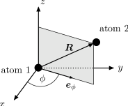
Figure 5: The atoms are aligned in a plane spanned by the unit vectors $\boldsymbol{e}_{z}$ and $\boldsymbol{e}_{\phi}=(\cos\phi,\sin\phi,0)$. Within this plane, the relative position of the two atoms $\boldsymbol{R}=z\,\boldsymbol{e}_{z}+l\,\boldsymbol{e}_{\phi}$ is described by the parameters $z$ and $l$. The energies of the eigenstates of $H_{A}+H_{\Omega}$ depend only on $z$ and $l$, but not on $\phi$.

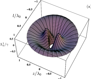
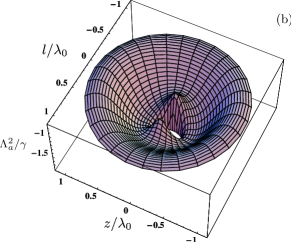
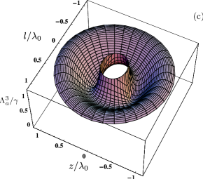
Figure 6: (Color online) Plot of the energy shifts that determine the energy levels of the antisymmetric states according to Eq. (54). In (a)-(c), the parameters $\Lambda_{a}^{i}$ are shown in a plane spanned by $\boldsymbol{e}_{z}$ and $\boldsymbol{e}_{\phi}=(\cos\phi,\sin\phi,0)$. The relative position $\boldsymbol{R}=z\,\boldsymbol{e}_{z}+l\,\boldsymbol{e}_{\phi}$ of the atoms in this plane is parameterized by $z$ and $l$ (see also Fig. 5). Since the $\Lambda_{a}^{i}$ do not depend on $\phi$, the energy surfaces shown in (a)-(c) do not change if $\boldsymbol{e}_{\phi}$ is rotated around the $z$-axis. While $\Lambda_{a}^{1}$ and $\Lambda_{a}^{2}$ tend to $-\infty$ in the limit $R\rightarrow 0$, $\Lambda_{a}^{3}$ tends to $+\infty$. The frequency splitting of the excited states is $\delta=\gamma$. In (d), the $\Lambda_{a}^{i}$ are shown as a function of the interatomic distance $R$, the parameters are $\theta=\pi/2$ and $\delta=\gamma$.

Figure 4(a) shows the parameters $\Gamma_{a}^{i}$ as a function of $R$. The oscillations of $\Gamma_{a}^{1}$ and $\Gamma_{a}^{2}$ around $\gamma$ are damped with $1/R$ as $R$ increases, and those of $\Gamma_{a}^{3}$ decrease with $1/R^{2}$. Note that the oscillations of the frequency shifts $\lambda_{a}^{i}$ display similar features for $R\gg\lambda_{0}$ (see Sec. IV.1). It has been shown in Sec. III that any state within the subspace $\mathcal{A}$ of antisymmetric states is completely stable for $R\rightarrow 0$. Consequently, the decay rates $2\Gamma_{a}^{i}$ of the states $|\psi_{a}^{i}\rangle$ tend to zero as $R$ approaches zero. It can be verified by numerical methods that $\Gamma_{a}^{1}$ and $\Gamma_{a}^{2}$ are smaller than the parameter $\gamma$ provided that $R\lesssim 0.44\times\lambda_{0}$, and $\Gamma_{a}^{3}$ does not exceed $\gamma$ if $R\lesssim 0.72\times\lambda_{0}$. For $R=0.1\times\lambda_{0}$, the coefficients $\Gamma_{a}^{i}$ are smaller than $0.1\times\gamma$. Although $R$ is larger than zero in an experiment, the states $|\psi_{a}^{i}\rangle$ decay much slower as compared to two non-interacting atoms if $R$ is sufficiently small. This shows that spontaneous emission can be strongly suppressed within the subspace $\mathcal{A}$ of the antisymmetric states, even for a realistic value of the interatomic distance $R$.

The parameters $\Gamma_{s}^{i}$ are depicted in Fig. 4(b). In the limit $R\rightarrow 0$, the coefficients $\Gamma_{s}^{i}$ tend to $2\gamma$. The symmetric states within the subspace $\mathcal{S}$ display thus superradiant features since they decay faster as compared to two independent atoms.

IV.3 Non-degenerate System

Here we discuss the diagonalization of $H_{A}+H_{\Omega}$ in the most general case where the Zeeman splitting $\delta$ of the excited states is different from zero. The matrix representation of this Hamiltonian with respect to the states $\{|\psi_{a}^{1}\rangle,|\psi_{a}^{2}\rangle,|\psi_{a}^{3}\rangle\}$ defined in Eq. (41) reads

$$[H_{A}+H_{\Omega}]_{\mathcal{A}} =\hbar\left(\begin{array}[]{l@{\hspace{0.3cm}}l@{\hspace{0.3cm}}l}\omega_{0}+\Omega_{F}\hfil\hskip 8.5359pt&\delta\cos\theta\hfil\hskip 8.5359pt&0\\ \delta\cos\theta\hfil\hskip 8.5359pt&\omega_{0}+\Omega_{F}\hfil\hskip 8.5359pt&-\delta\sin\theta\\ 0\hfil\hskip 8.5359pt&-\delta\sin\theta\hfil\hskip 8.5359pt&\omega_{0}+\Omega_{N}\end{array}\right)\,.$$ (53)

Figure 7: Complete level scheme of the non-degenerate system ($\delta\not=0$). For the special geometrical setup where the atoms are aligned in the $x$-$y$-plane ($\theta=\pi/2$), the analytical expressions for the states $|\varphi_{a}^{i}\rangle$, $|\varphi_{s}^{i}\rangle$ and the frequency shifts $\Lambda_{a}^{i}$, $\Lambda_{s}^{i}$ are given in Eqs. (57), (65), (55) and (64), respectively. The frequency shifts $\Lambda_{a}^{i}$ ($\Lambda_{s}^{i}$) of the antisymmetric (symmetric) states and the splitting of the excited states are not to scale. Note that the frequency shifts $\Lambda_{a}^{i}$ and $\Lambda_{s}^{i}$ depend on the relative position of the atoms.

In general, the eigenvalues of this matrix can be written in the form

$$E_{a}^{1} = \hbar\left(\omega_{0}+\Lambda_{a}^{1}\right)\,,$$

$$E_{a}^{2} = \hbar\left(\omega_{0}+\Lambda_{a}^{2}\right)\,,$$

$$E_{a}^{3} = \hbar\left(\omega_{0}+\Lambda_{a}^{3}\right)\,,$$ (54)

where the frequency shifts $\Lambda_{a}^{i}$ depend only on the interatomic distance $R$ and the azimuthal angle $\theta$, but not on the angle $\phi$. To illustrate this result, we consider a plane spanned by $\boldsymbol{e}_{z}$ and $\boldsymbol{e}_{\phi}=(\cos\phi,\sin\phi,0)$, see Fig. 5. Within this plane, the vector $\boldsymbol{R}=z\,\boldsymbol{e}_{z}+l\,\boldsymbol{e}_{\phi}$ is described by the parameters $z$ and $l$, and Fig. 6(a)-(c) shows $\Lambda_{a}^{i}(l,z)$ as a function of these variables. Since the $\Lambda_{a}^{i}$ do not depend on $\phi$, the energy surfaces shown in Fig. 6(a)-(c) remain the same if $\boldsymbol{e}_{\phi}$ is rotated around the $z$-axis. This result follows from the fact that the Hamiltonian $H_{A}$ in Eq. (2) is invariant under rotations around the $z$- axis kif .

In Sec. VI, we will focus on the geometrical setup where the atoms are aligned in the $x$- $y$- plane ($\theta=\pi/2$). In this case, the frequency shifts $\Lambda_{a}^{i}$ of the antisymmetric states are found to be

$$\Lambda_{a}^{1} = \Omega_{F}\,,$$

$$\Lambda_{a}^{2} = (\Omega_{F}+\Omega_{N})/2-\omega_{B}/2\,,$$

$$\Lambda_{a}^{3} = (\Omega_{F}+\Omega_{N})/2+\omega_{B}/2\,,$$ (55)

where the Bohr frequency is given by

$$\omega_{B}=\sqrt{4\delta^{2}+(\Omega_{F}-\Omega_{N})^{2}}\,.$$ (56)

A plot of the frequency shifts $\Lambda_{a}^{i}$ as a function of the interatomic distance $R$ and for $\theta=\pi/2$ is shown in Fig. 6(d). Note that the degeneracy and the level crossing of the eigenvalues $\lambda_{a}^{i}$ is removed for $\delta\not=0$ [see Sec. IV.1]. The eigenstates that correspond to the frequency shifts in Eq. (55) read

$$|\varphi_{a}^{1}\rangle = |a_{2}\rangle\,,$$

$$|\varphi_{a}^{2}\rangle = e^{i\xi}\sin\vartheta_{a}|\psi_{a}^{+}\rangle+\cos\vartheta_{a}|\psi_{a}^{-}\rangle\,,$$

$$|\varphi_{a}^{3}\rangle = -e^{i\xi}\cos\vartheta_{a}|\psi_{a}^{+}\rangle+\sin\vartheta_{a}|\psi_{a}^{-}\rangle\,,$$ (57)

where $\delta=|\delta|e^{i\xi}$ ($\xi\in\{0,\pi\}$), the states $|\psi_{a}^{\pm}\rangle$ are defined in Eq. (42), and the angle $\vartheta_{a}$ is determined by

$$\tan 2\vartheta_{a}=\frac{|\delta|}{\Omega_{F}-\Omega_{N}}\,,\quad 0<\vartheta_{a}<\frac{\pi}{2}\,.$$ (58)

If the distance between the atoms is small such that $R\lesssim 0.63\times\lambda_{0}$, we have $\Omega_{F}<\Omega_{N}$. In this case, we find $\lim_{\delta\rightarrow 0}|\varphi_{a}^{i}\rangle=|\psi_{a}^{i}\rangle$ and $\lim_{\delta\rightarrow 0}\Lambda_{a}^{i}=\lambda_{a}^{i}$, where the eigenstates $|\psi_{a}^{i}\rangle$ and the frequency shifts $\lambda_{a}^{i}$ of the degenerate system are defined in Eqs. (41) and (43), respectively.

The matrix representation of $H_{A}+H_{\Omega}$ with respect to the symmetric states $\{|\psi_{s}^{1}\rangle,|\psi_{s}^{2}\rangle,|\psi_{s}^{3}\rangle\}$ defined in Eq. (45) is found to be

$$[H_{A}+H_{\Omega}]_{\mathcal{S}} =\hbar\left(\begin{array}[]{l@{\hspace{0.3cm}}l@{\hspace{0.3cm}}l}\omega_{0}-\Omega_{F}\hfil\hskip 8.5359pt&\delta\cos\theta\hfil\hskip 8.5359pt&0\\ \delta\cos\theta\hfil\hskip 8.5359pt&\omega_{0}-\Omega_{F}\hfil\hskip 8.5359pt&-\delta\sin\theta\\ 0\hfil\hskip 8.5359pt&-\delta\sin\theta\hfil\hskip 8.5359pt&\omega_{0}-\Omega_{N}\end{array}\right)\,.$$ (62)

Just as in the case of the antisymmetric states, the eigenvalues of $[H_{A}+H_{\Omega}]_{\mathcal{S}}$ are written as

$$E_{s}^{1} = \hbar\left(\omega_{0}+\Lambda_{s}^{1}\right)\,,$$

$$E_{s}^{2} = \hbar\left(\omega_{0}+\Lambda_{s}^{2}\right)\,,$$

$$E_{s}^{3} = \hbar\left(\omega_{0}+\Lambda_{s}^{3}\right)\,,$$ (63)

and the frequency shifts $\Lambda_{s}^{i}$ depend only on the interatomic distance $R$ and the azimuthal angle $\theta$.

If the atoms are aligned in the $x$- $y$- plane ($\theta=\pi/2$), the frequency shifts $\Lambda_{s}^{i}$ of the symmetric states are given by

$$\Lambda_{s}^{1} = -\Omega_{F}\,,$$

$$\Lambda_{s}^{2} = -(\Omega_{F}+\Omega_{N})/2+\omega_{B}/2\,,$$

$$\Lambda_{s}^{3} = -(\Omega_{F}+\Omega_{N})/2-\omega_{B}/2\,,$$ (64)

and the corresponding eigenstates are

$$|\varphi_{s}^{1}\rangle = |s_{2}\rangle\,,$$

$$|\varphi_{s}^{2}\rangle = -e^{i\xi}\cos\vartheta_{s}|\psi_{s}^{+}\rangle+\sin\vartheta_{s}|\psi_{s}^{-}\rangle\,,$$

$$|\varphi_{s}^{3}\rangle = e^{i\xi}\sin\vartheta_{s}|\psi_{s}^{+}\rangle+\cos\vartheta_{s}|\psi_{s}^{-}\rangle\,.$$ (65)

The states $|\psi_{s}^{\pm}\rangle$ are defined in Eq. (46), $\delta=|\delta|e^{i\xi}$ ($\xi\in\{0,\pi\}$), and the angle $\vartheta_{s}$ is determined by

$$\tan 2\vartheta_{s}=\frac{|\delta|}{\Omega_{N}-\Omega_{F}}\,,\quad 0<\vartheta_{s}<\frac{\pi}{2}\,.$$ (66)

For small values of the interatomic distance $R$ such that $\Omega_{F}<\Omega_{N}$, we find $\lim_{\delta\rightarrow 0}|\varphi_{s}^{i}\rangle=|\psi_{s}^{i}\rangle$ and $\lim_{\delta\rightarrow 0}\Lambda_{s}^{i}=\lambda_{s}^{i}$, where the eigenstates $|\psi_{s}^{i}\rangle$ and the frequency shifts $\lambda_{s}^{i}$ of the degenerate system are defined in Eqs. (45) and (47), respectively.

Finally, we note that the ground state $|4,4\rangle$ and the excited states $|i,j\rangle$ ($i,j\in\{1,2,3\}$) are eigenstates of $H_{A}+H_{\Omega}$. These states together with the symmetric and antisymmetric eigenstates of $H_{A}+H_{\Omega}$ form the new basis of the total state space $\mathcal{H}_{\text{sys}}$. The complete level scheme of the non-degenerate system is shown in Fig. 7.

V POPULATION OF THE DECOHERENCE FREE SUBSPACE

In this section we describe a method that allows to populate the subspace $\mathcal{A}$ spanned by the antisymmetric states. For simplicity, we restrict the analysis to the degenerate system ($\delta=0$) and show how the states $|\psi_{a}^{i}\rangle$ can be populated selectively by means of an external laser field. However, a laser field cannot induce direct transitions between the ground state $|4,4\rangle$ and $|\psi_{a}^{i}\rangle$ as long as the electric field at the position of atom 1 is identical to the field at the location of atom 2. By contrast, a direct driving of the antisymmetric states is possible provided that one can realize a field gradient between the positions of the two atoms. Since we consider an interatomic spacing $R$ that is smaller than $\lambda_{0}/2$ such that the states in $\mathcal{A}$ are subradiant, the realization of this field gradient is an experimentally challenging task. Several authors proposed a setup where the atoms are placed symmetrically around the node of a standing light field Ficek and Tanaś (2002); Beige et al. (2000), and this method also allows to address the states of our system individually. Other methods Akram et al. (2000); Ficek and Swain (2005); Ficek and Tanaś (2002) rest on the assumption that the atoms are non-identical and cannot be applied to our system comprised of two identical atoms.

	$|\psi_{a}^{1}\rangle$	$|\psi_{a}^{2}\rangle$	$|\psi_{a}^{3}\rangle$
$|1,2\rangle$	$\boldsymbol{e}_{x},\,\boldsymbol{e}_{y}$	$\boldsymbol{e}_{z}$	$\boldsymbol{e}_{z}$
$|2,1\rangle$	$\boldsymbol{e}_{x},\,\boldsymbol{e}_{y}$	$\boldsymbol{e}_{z}$	$\boldsymbol{e}_{z}$
$|1,3\rangle$	-	$\boldsymbol{e}_{x}$	$\boldsymbol{e}_{y}$
$|3,1\rangle$	-	$\boldsymbol{e}_{x}$	$\boldsymbol{e}_{y}$
$|2,3\rangle$	$\boldsymbol{e}_{x},\,\boldsymbol{e}_{y}$	$\boldsymbol{e}_{z}$	$\boldsymbol{e}_{z}$
$|3,2\rangle$	$\boldsymbol{e}_{x},\,\boldsymbol{e}_{y}$	$\boldsymbol{e}_{z}$	$\boldsymbol{e}_{z}$

Table 1: Polarization of the external laser field that couples an antisymmetric state $|\psi_{a}^{i}\rangle$ to an excited state $|i,j\rangle$ ($i,j\in\{1,2,3\}$) for $\delta=0$. Note that $|\psi_{a}^{1}\rangle$ does not couple to $z$-polarized light, $|\psi_{a}^{2}\rangle$ does not couple to $y$-polarized light and $|\psi_{a}^{1}\rangle$ does not couple to $x$-polarized light. See also Fig. 8.

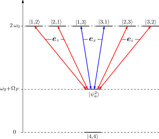
Figure 8: (Color online) Laser-induced coupling of $|\psi_{a}^{2}\rangle$ to the excited states $|i,j\rangle$ ($i,j\in\{1,2,3\}$) in the case of the degenerate system. States that are not directly coupled to $|\psi_{a}^{2}\rangle$ have been omitted (except for the ground state). The laser polarization that couples the antisymmetric state $|\psi_{a}^{2}\rangle$ to a state $|i,j\rangle$ ($i,j\in\{1,2,3\}$) is indicated next to the respective transition. $|\psi_{a}^{2}\rangle$ is completely decoupled from a $y$-polarized laser field.

Here we describe a method that allows to populate the states $|\psi_{a}^{i}\rangle$ individually and that does not require a field gradient between the positions of the two atoms. It rests on a finite distance between the atoms and exploits the fact that the antisymmetric states may be populated by spontaneous emission from the excited states $|i,j\rangle$ ($i,j\in\{1,2,3\}$). For a given geometrical setup, we choose a coordinate system where the unit vector $\boldsymbol{e}_{x}$ coincides with the separation vector $\boldsymbol{R}$. In this case, we have $\theta=\pi/2$ and $\phi=0$. The $z$-direction is determined by the external magnetic field and can be chosen in any direction perpendicular to $\boldsymbol{R}$. The polarization vector of the laser field propagating in $z$-direction lies in the $x$-$y$-plane and can be adjusted as needed, see Eq. (17). In the presence of the laser, the atomic evolution is governed by the master equation (18). We find that the coupling of the states $|\psi_{a}^{i}\rangle$ to the excited states $|i,j\rangle$ ($i,j\in\{1,2,3\}$) depends on the polarization of the laser field (see Table 1 and Fig. 8). In particular, it is found that $|\psi_{a}^{1}\rangle$ does not couple to $z$-polarized light, $|\psi_{a}^{2}\rangle$ does not couple to $y$-polarized light and $|\psi_{a}^{3}\rangle$ does not couple to $x$-polarized light. At the same time, the states $|\psi_{a}^{i}\rangle$ are populated by spontaneous emission from the excited states. This fact together with the polarization dependent coupling of the antisymmetric states allows to populate the states $|\psi_{a}^{i}\rangle$ selectively. In order to populate state $|\psi_{a}^{2}\rangle$, for example, one has to shine in a $y$-polarized field. Since the spontaneous decay of $|\psi_{a}^{2}\rangle$ is slow and since $|\psi_{a}^{2}\rangle$ is decoupled from the laser, population can accumulate in this state. On the other hand, the states $|\psi_{a}^{1}\rangle$ and $|\psi_{a}^{3}\rangle$ are depopulated by the laser coupling to the excited states. This situation is shown in Fig. 9(a) for two different values of the interatomic distance $R$. The initial state at $t=0$ is $|4,4\rangle$, and for $t\cdot\gamma=20$ the population of $|\psi_{a}^{2}\rangle$ is approximately 1/4. Since all coherences between $|\psi_{a}^{2}\rangle$ and any other state are zero, the probability to find the system at $t=20/\gamma$ in the pure state $|\psi_{a}^{2}\rangle$ is given by 1/4.

The exact steady state solution of Eq. (18) is difficult to obtain analytically. However, one can determine the steady state value of $\langle\psi_{a}^{2}|\varrho|\psi_{a}^{2}\rangle$ with the help of Eq. (48),

$$\langle\psi_{a}^{2}|\varrho_{\text{st}}|\psi_{a}^{2}\rangle=\left[\lim\limits_{t\rightarrow\infty}C_{a}^{2}(t)\right]/(2\Gamma_{a}^{2})\,.$$ (67)

The population of $|\psi_{a}^{2}\rangle$ in steady state is thus limited by the population of the relevant excited states that are populated by the $y$-polarized laser field and that decay spontaneously to $|\psi_{a}^{2}\rangle$. Furthermore, it is possible to gain some insight into the time evolution of $\langle\psi_{a}^{2}|\varrho|\psi_{a}^{2}\rangle$. For a strong laser field and for a small value of $R$, $C_{a}^{2}$ reaches the steady state on a timescale that is fast as compared to $1/(2\Gamma_{a}^{2})$. We may thus replace $C_{a}^{2}$ by its steady state value in Eq. (48). The solution of this differential equation is

$$\langle\psi_{a}^{i}|\varrho(t)|\psi_{a}^{i}\rangle\approx\frac{\left[\lim\limits_{t\rightarrow\infty}C_{a}^{i}(t)\right]}{2\Gamma_{a}^{i}}\left[1-e^{-2\Gamma_{a}^{2}t}\right]$$ (68)

and reproduces the exact time evolution of $\langle\psi_{a}^{2}|\varrho|\psi_{a}^{2}\rangle$ according to Fig. 9(a) quite well. Moreover, it becomes now clear why it takes longer until the population of $|\psi_{a}^{2}\rangle$ reaches its steady state if the interatomic distance $R$ is reduced since the decay rate $2\Gamma_{a}^{2}$ approaches zero as $R\rightarrow 0$.

Figure 9: Time-dependent population of the states $|\psi_{a}^{i}\rangle$ for different polarizations of the driving field. The initial state at $t=0$ is $|4,4\rangle$. The parameters are $\theta=\pi/2$, $\phi=0$, $\delta=0$ and $\Delta_{2}=0$. (a) Population of $|\psi_{a}^{2}\rangle$ for $\Omega_{y}(\boldsymbol{r}_{1})=\Omega_{y}(\boldsymbol{r}_{2})=5\gamma$. The states $|\psi_{a}^{1}\rangle$ and $|\psi_{a}^{3}\rangle$ are not populated. (b) Population of $|\psi_{a}^{3}\rangle$ for $\Omega_{x}(\boldsymbol{r}_{1})=\Omega_{x}(\boldsymbol{r}_{2})=5\gamma$. The states $|\psi_{a}^{1}\rangle$ and $|\psi_{a}^{2}\rangle$ are not populated.

So far, we considered only the population of $|\psi_{a}^{2}\rangle$, but the treatment of $|\psi_{a}^{1}\rangle$ and $|\psi_{a}^{3}\rangle$ is completely analogous. The population of $|\psi_{a}^{3}\rangle$ by a $x$-polarized field is shown in Fig. 9(b). The differences between plot (a) and (b) arise since the decay rates of $|\psi_{a}^{2}\rangle$ and $|\psi_{a}^{3}\rangle$ are different for the same value of $R$ (see Sec. IV.2). In general, the presented method may also be employed to populate the antisymmetric states of the non-degenerate system selectively. In this case, the polarization of the field needed to populate a state $|\varphi_{a}^{i}\rangle$ is a function of the detuning $\delta$.

In conclusion, the discussed method allows to populate the antisymmetric states selectively, provided that the interatomic distance is larger than zero. If the interatomic distance is reduced, a longer interaction time with the laser field is required to reach the maximal value of $\langle\psi_{a}^{i}|\varrho|\psi_{a}^{i}\rangle\approx 1/4$. Note that a finite distance between the atoms is also required in the case of other schemes where the atoms are placed symmetrically around the node of a standing light field Ficek and Tanaś (2002); Beige et al. (2000). While the latter method allows, at least in principle, for a complete population transfer to the antisymmetric states, its experimental realization is difficult for two nearby atoms. By contrast, our scheme does not require a field gradient between the atoms and is thus easier to implement. It has been pointed out that the population transfer to the antisymmetric states is limited by the population of the excited states that spontaneously decay to an antisymmetric state $|\psi_{a}^{i}\rangle$. Although this limit is difficult to overcome, an improvement can be achieved if the fluorescence intensity is observed while the atom is irradiated by the laser. As soon as the system decays into one of the states $|\psi_{a}^{i}\rangle$, the fluorescence signal is interrupted for a time period that is on the order of $1/(2\Gamma_{a}^{i})$ (see Sec. IV.2). The dark periods in the fluorescence signal reveal thus the spontaneous emission events that lead to the population of one of the antisymmetric states.

VI INDUCING DYNAMICS WITHIN THE SUBSPACE $\mathcal{A}$

In this Section we assume that the system has been prepared in the antisymmetric state $|\psi_{a}^{2}\rangle$, for example by one of the methods described in Sec. V. The aim is to induce a controlled dynamics in the subspace $\mathcal{A}$ of the antisymmetric states. We suppose that the atoms are aligned along the $x$-axis, i.e. $\theta=\pi/2$ and $\phi=0$. According to Eq. (53), the state $|\psi_{a}^{2}\rangle$ is then only coupled to $|\psi_{a}^{3}\rangle$. Apart from a constant, the Hamiltonian $H_{\mathcal{Q}}$ that governs the unitary time evolution in the space $\mathcal{Q}$ spanned by $\{|\psi_{a}^{2}\rangle,\,|\psi_{a}^{3}\rangle\}$ can be written as

$$H_{\mathcal{Q}} =\hbar\left(\begin{array}[]{l@{\hspace{0.3cm}}l }-(\Omega_{N}-\Omega_{F})/2\hfil\hskip 8.5359pt&-\delta\\ -\delta\hfil\hskip 8.5359pt&(\Omega_{N}-\Omega_{F})/2\end{array}\right)$$ (71)

$$=\hbar\omega_{B}\boldsymbol{\hat{n}}\cdot\boldsymbol{\sigma}/2\,,$$ (72)

where the vector $\boldsymbol{\sigma}=\{\sigma_{x},\sigma_{y},\sigma_{z}\}$ consists of the Pauli matrices $\sigma_{i}$, and the unit vector $\boldsymbol{\hat{n}}$ is defined as

$$\boldsymbol{\hat{n}}=-\left(2\delta,0,\Omega_{N}-\Omega_{F}\right)/\omega_{B}\,.$$ (73)

The Bohr frequency $\omega_{B}$ is the difference between the eigenvalues of $H_{\mathcal{Q}}$ and is given in Eq. (56) of Sec. IV.3. Equation (72) implies that the parameter $\delta$ which can be adjusted by means of the external magnetic field introduces a coupling between the states $|\psi_{a}^{2}\rangle$ and $|\psi_{a}^{3}\rangle$. If the initial state is $|\psi_{a}^{2}\rangle$, the final state $|\psi_{F}\rangle$ reads

$$|\psi_{F}(t)\rangle=U(t,0)|\psi_{a}^{2}\rangle,\,$$ (74)

where $U=\exp(-iH_{\mathcal{Q}}t/\hbar)$ is the time evolution operator. The time evolution induced by $H_{\mathcal{Q}}$ can be described in a simple way in the Bloch sphere picture Nielsen and Chuang (2000). The Bloch vector of the state $|\psi_{F}(t)\rangle$ is defined as

$$\boldsymbol{B}(t)=\langle\psi_{F}(t)|\boldsymbol{\sigma}|\psi_{F}(t)\rangle\,.$$ (75)

Initially, this vector points into the positive $z$-direction. The time evolution operator $U$ rotates this vector on the Bloch sphere around the axis $\boldsymbol{\hat{n}}$ by an angle $\omega_{B}t$. According to Eq. (73), the axis of rotation lies in the $x$-$z$-plane and its orientation depends on the parameter $\delta$ which can be controlled by means of the magnetic field. In order to demonstrate these analytical considerations, we numerically integrate the master equation (7) with the initial condition $\varrho(t=0)=|\psi_{a}^{2}\rangle\langle\psi_{a}^{2}|$. We define a projector onto the space spanned by $\{|\psi_{a}^{2}\rangle,\,|\psi_{a}^{3}\rangle\}$,

$$\hat{P}=|\psi_{a}^{2}\rangle\langle\psi_{a}^{2}|+|\psi_{a}^{3}\rangle\langle\psi_{a}^{3}|\,.$$ (76)

The generalized Bloch vector is then defined as

$$\boldsymbol{B}_{N}(t)=\text{Tr}\left[\boldsymbol{\sigma}\hat{P}\varrho(t)\hat{P}\right]\,.$$ (77)

In contrast to $\boldsymbol{B}$, $\boldsymbol{B}_{N}$ is not necessarily a unit vector, but its length can be smaller than unity due to spontaneous emission from $|\psi_{a}^{2}\rangle$ and $|\psi_{a}^{3}\rangle$ to the ground state. Figure 10 shows the evolution of $\boldsymbol{B}_{N}$ for different values of the parameter $\delta$ which depends on the magnetic field strength. Let $\boldsymbol{S}=\{S_{x},S_{y},S_{z}\}$ be a point on the Bloch sphere that lies not in the $y$-$z$-plane ($S_{x}\not=0$). If one chooses the parameter $\delta$ according to

$$\delta=\frac{1-S_{z}}{2|S_{x}|}|\Omega_{F}-\Omega_{N}|\;\text{Sign}(S_{x})\,,$$ (78)

then $\boldsymbol{S}$ lies on the orbit of the rotating Bloch vector $\boldsymbol{B}$ if spontaneous emission is negligible. According to Eq. (78), any point close to the $y$-$z$-plane requires large values of $\delta$ since $|\delta|$ diverges for $S_{x}\rightarrow 0$. The dynamics that can be induced by a static magnetic field is thus restricted, particularly because we are only considering the regime of the linear Zeeman effect.

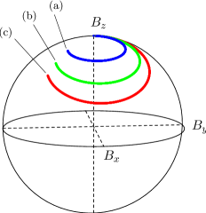
Figure 10: (Color online) Bloch sphere representation of the system dynamics in the subspace $\mathcal{Q}$ spanned by the states $\{|\psi_{a}^{2}\rangle,\,|\psi_{a}^{3}\rangle\}$. At $t=0$, the system is in the pure state $|\psi_{a}^{2}\rangle$ and a static magnetic field is switched on. The Bloch vector is rotated around an axis in the $x$-$z$-plane, and the tilt of this axis in $x$-direction increases with the magnetic field strength. The value of the parameter $\delta$ is (a) $\delta=3.15\times\gamma$, (b) $\delta=4.83\times\gamma$ and (c) $\delta=6.22\times\gamma$, and we chose $R=0.1\times\lambda_{0}$.

These limitations can be overcome if a radio-frequency (RF) field is applied instead of a static magnetic field. If the RF field oscillates along the $z$-axis, the Hamiltonian $H_{A}$ in Eq. (2) has to be replaced by

$$H_{A}^{\text{rf}}(t)=\hbar\omega_{0}\sum\limits_{i=1}^{3}\sum\limits_{\mu=1}^{2}\,S_{i\,+}^{(\mu)}S_{i\,-}^{(\mu)}+V_{\text{rf}}(t)\,,$$ (79)

where

$$V_{\text{rf}}(t)=2\hbar\delta(t)\sum\limits_{\mu=1}^{2}\,\left(S_{3\,+}^{(\mu)}S_{3\,-}^{(\mu)}-S_{1\,+}^{(\mu)}S_{1\,-}^{(\mu)}\right)$$ (80)

describes the interaction with the RF field and

$$\delta(t)=\delta_{0}\cos(\omega_{\text{rf}}\,t+\phi_{\text{rf}})\,.$$ (81)

In this equation, the magnitude of $\delta_{0}(>0)$ depends on the amplitude of the RF field, and $\omega_{\text{rf}}$ and $\phi_{\text{rf}}$ are the frequency and phase of the RF field, respectively. We assume that the interatomic distance of the atoms is smaller than $R=0.63\times\lambda_{0}$. In this case, the dipole-dipole interaction raises the energy of $|\psi_{a}^{3}\rangle$ with respect to $|\psi_{a}^{2}\rangle$, and the frequency difference between these two states is $\Omega_{N}-\Omega_{F}>0$. Furthermore, we suppose that the detuning $\Delta_{\text{rf}}=\omega_{\text{rf}}-(\Omega_{N}-\Omega_{F})$ of the RF field with the $|\psi_{a}^{2}\rangle\leftrightarrow|\psi_{a}^{3}\rangle$ transition and the parameter $\delta_{0}$ are small as compared to $(\Omega_{N}-\Omega_{F})$ such that the rotating-wave approximation can be employed. In a frame rotating with $\omega_{\text{rf}}$, the system dynamics in the subspace $\mathcal{Q}$ spanned by $\{|\psi_{a}^{2}\rangle,\,|\psi_{a}^{3}\rangle\}$ is then governed by the Hamiltonian

$$H_{\mathcal{Q}}^{\text{rf}} =\hbar\left(\begin{array}[]{l@{\hspace{0.3cm}}l }\Delta_{\text{rf}}/2\hfil\hskip 8.5359pt&-\delta_{0}\exp(i\phi_{\text{rf}})\\[5.69046pt] -\delta_{0}\exp(-i\phi_{\text{rf}})\hfil\hskip 8.5359pt&-\Delta_{\text{rf}}/2\end{array}\right)$$ (84)

$$=\hbar\Omega_{\text{rf}}\,\boldsymbol{\hat{n}}_{\text{rf}}\cdot\boldsymbol{\sigma}/2\,,$$ (85)

where

$$\boldsymbol{\hat{n}}_{\text{rf}}=\left(-2\delta_{0}\cos\phi_{\text{rf}},-2\delta_{0}\sin\phi_{\text{rf}},\Delta_{\text{rf}}\right)/\Omega_{\text{rf}}$$ (86)

and $\Omega_{\text{rf}}=\sqrt{\Delta_{\text{rf}}^{2}+4|\delta_{0}|^{2}}$. For a resonant RF field ($\Delta_{\text{rf}}=0$), the axis $\boldsymbol{\hat{n}}_{\text{rf}}$ lies in the $x$-$y$-plane of the Bloch sphere, and its orientation can be adjusted at will by the phase $\phi_{\text{rf}}$ of the RF field. Any single-qubit operation can thus be realized by a sequence of suitable RF pulses Nielsen and Chuang (2000). In particular, a complete transfer of population from $|\psi_{a}^{2}\rangle$ to $|\psi_{a}^{3}\rangle$ can be achieved by a resonant RF pulse with a duration of $\pi/\Omega_{\text{rf}}$ and an arbitrary phase $\phi_{\text{rf}}$.

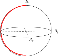
Figure 11: (Color online) Complete population transfer from $|\psi_{a}^{2}\rangle$ to $|\psi_{a}^{3}\rangle$ by means of a resonant RF field. At $t=0$, the Bloch vector $\boldsymbol{B}_{N}$ points into the positive $z$ direction. At $t=\pi/\Omega_{\text{rf}}$, the state of the system is $|\psi_{a}^{3}\rangle$ and $\boldsymbol{B}_{N}$ points into the negative $z$ direction. Note that the length of $\boldsymbol{B}_{N}$ is slightly smaller than unity for $t>0$ due to the small probability of spontaneous emission to the ground state. The parameters are $R=0.05\times\lambda_{0}$, $\delta_{0}=\gamma$, $\phi_{\text{rf}}=\pi$ and $\Delta_{\text{rf}}=0$.

Next we demonstrate that the Hamiltonian $H_{\mathcal{Q}}^{\text{rf}}$ in Eq. (85) describes the system dynamics quite well if the atoms are close to each other such that spontaneous emission is strongly suppressed. For this, we transform the master equation (7) with $H_{A}^{\text{rf}}$ instead of $H_{A}$ in a frame rotating with $\omega_{\text{rf}}$. The resulting equation is integrated numerically without making the rotating-wave approximation. We suppose that the system is initially in the state $|\psi_{a}^{2}\rangle$, and the phase of the resonant RF field has been set to $\phi_{\text{rf}}=\pi$. Figure 11 shows the time evolution of the Bloch vector $\boldsymbol{B}_{N}$. As predicted by Eq. (85), the Bloch vector is rotated around the $x$-axis and at $t=\pi/\Omega_{\text{rf}}$, $\boldsymbol{B}_{N}$ points in the negative $z$-direction. Due to the small probability of spontaneous emission to the ground state, the length of $\boldsymbol{B}_{N}$ is slightly smaller than unity ($|\boldsymbol{B}_{N}|=0.95$) at $t=\pi/\Omega_{\text{rf}}$.

Finally, we briefly discuss how the final state $|\psi_{F}(t)\rangle$ could be measured. In principle, one can exploit the polarization-dependent coupling of the states $|\psi_{a}^{2}\rangle$ and $|\psi_{a}^{3}\rangle$ to the excited states (see Sec. V). For example, one could ionize the system in a two-step process, where $|\psi_{a}^{2}\rangle$ ($|\psi_{a}^{3}\rangle$) is first resonantly coupled to the excited states $|i,j\rangle$ ($i,j\in\{1,2,3\}$). A second laser then ionizes the system, and the ionization rate is a measure for the population of state $|\psi_{a}^{2}\rangle$ ($|\psi_{a}^{3}\rangle$). Another possibility is to shine in a single laser whose frequency is just high enough to ionize the system starting from $|\psi_{a}^{3}\rangle$. Since the energy of $|\psi_{a}^{3}\rangle$ is higher than those of $|\psi_{a}^{2}\rangle$, the ionization rate is a measure for the population of state $|\psi_{a}^{3}\rangle$.

VII ENTANGLEMENT OF THE COLLECTIVE TWO-ATOM STATES

In Sec. IV.1, we determined the collective two-atom states $|\psi_{a}^{i}\rangle$ and $|\psi_{s}^{i}\rangle$ that are formed by the coherent part of the dipole-dipole interaction. Here we show that these states are entangled, i.e. they cannot be written as a single tensor product $|\psi_{1}\rangle\otimes|\psi_{2}\rangle$ of two single-atom states. In order to quantify the degree of entanglement, we calculate the concurrence Wootters (1998); Rungta et al. (2001) of the pure states $|\psi_{a}^{i}\rangle$ and $|\psi_{s}^{i}\rangle$. The concurrence for a pure state $|\psi_{12}\rangle$ of the two-atom state space $\mathcal{H}_{\text{sys}}=\mathcal{H}_{1}\otimes\mathcal{H}_{2}$ is defined as Rungta et al. (2001)

$$C(|\psi_{12}\rangle)=\sqrt{2[1-\text{Tr}(\varrho_{1}^{2})]}\,.$$ (87)

Here $\varrho_{1}=\text{Tr}_{2}(\varrho)$ denotes the reduced density operator of atom 1. The concurrence $C$ of a maximally entangled state in $\mathcal{H}_{\text{sys}}$ is $C_{\text{max}}=\sqrt{3/2}$, and $C$ is zero for product states Rungta et al. (2001). We find that the antisymmetric and symmetric states $|\psi_{a}^{i}\rangle$ and $|\psi_{s}^{i}\rangle$ are entangled, but the degree of entanglement is not maximal,

$$C(|\psi_{a}^{i}\rangle)=C(|\psi_{s}^{i}\rangle)=1<C_{\text{max}}\,.$$ (88)

Next we compare this result to the corresponding results for a pair of interacting two-level systems with ground state $|g\rangle$ and excited state $|e\rangle$. In this case, the exchange interaction gives rise to the entangled states Dicke (1954); Ficek and Tanaś (2002); Ficek and Swain (2005)

$$|\pm\rangle=\frac{1}{\sqrt{2}}(|e,g\rangle\pm|g,e\rangle)$$ (89)

with $C(|\pm\rangle)=1$. It follows that the degree of entanglement of the states $|\pm\rangle$ is the same than the degree of entanglement of the symmetric and antisymmetric states of two four-level systems. On the other hand, the states $|\pm\rangle$ are maximally entangled in the state space of two two-level systems. This is in contrast to the states $|\psi_{a}^{i}\rangle$ and $|\psi_{s}^{i}\rangle$ which are not maximally entangled in the state space of two four-level atoms. Note that the system of two four-level atoms shown in Fig. 1 may be reduced to a pair of two-level systems if the atoms are aligned along the $z$-axis. For this particular setup, all cross-coupling terms $\Omega_{ij}$ and $\Gamma_{ij}$ with $i\not=j$ vanish [see Eqs. (15) and (16)] such that an arbitrary sublevel of the $P_{1}$ triplet and the ground state $S_{0}$ form an effective two-level system.

In Sec. VI, we showed that a static magnetic or RF field can induce a controlled dynamics between the states $|\psi_{a}^{2}\rangle$ and $|\psi_{a}^{3}\rangle$. We find that the degree of entanglement of an arbitrary superposition state

$$|\psi_{\text{sup}}\rangle=a|\psi_{a}^{2}\rangle+b|\psi_{a}^{3}\rangle$$ (90)

with $|a|^{2}+|b|^{2}=1$ is given by $C(|\psi_{\text{sup}}\rangle)=1$. It follows that the degree of entanglement is not influenced by the induced dynamics between the states $|\psi_{a}^{2}\rangle$ and $|\psi_{a}^{3}\rangle$.

Finally, we point out that the antisymmetric states $|\psi_{a}^{i}\rangle$ can be populated selectively, for example by the method introduced in Sec. V. Since the spontaneous decay of the antisymmetric states is suppressed if the interatomic distance is small as compared to mean transition wavelength $\lambda_{0}$, we have shown that the system can be prepared in long-lived entangled states.

VIII SUMMARY AND DISCUSSION

We have shown that the state space of two dipole-dipole interacting four-level atoms contains a four-dimensional decoherence-free subspace (DFS) if the interatomic distance approaches zero. If the separation of the atoms is larger than zero but small as compared to the wavelength of the $S_{0}\leftrightarrow P_{1}$ transition, the spontaneous decay of states within the DFS is suppressed. In addition, we have shown that the system dynamics within the DFS is closed, i.e., the coherent part of the dipole-dipole interaction does not introduce a coupling between states of the DFS and states outside of the DFS.

In the case of degenerate excited states ($\delta=0$), we find that the energy levels depend only on the interatomic distance $R$, but not on the angles $\theta$ and $\phi$. This result reflects the fact that each atom is modelled by complete sets of angular momentum multiplets kif . We identified two antisymmetric collective states ($|\psi_{a}^{2}\rangle$ and $|\psi_{a}^{3}\rangle$) within the DFS that can be employed to represent a qubit. The storing times of the qubit state depend on the interatomic distance $R$ and can be significantly longer than the inverse decay rate of the $S_{0}\leftrightarrow P_{1}$ transition. Moreover, any single-qubit operation can be realized via a sequence of suitable RF pulses. The energy splitting between the states $|\psi_{a}^{2}\rangle$ and $|\psi_{a}^{3}\rangle$ arises from the coherent dipole-dipole interaction between the atoms and is on the order of $10\gamma\equiv(10-1000)$ MHz in the relevant interatomic distance range. The coupling strength between the RF field and the atoms is characterized by the parameter $\delta_{0}$ which is on the order of $\mu_{B}B_{0}$, where $\mu_{B}$ is the Bohr magneton and $B_{0}$ is the amplitude of the RF field. Since $\mu_{B}$ is about $3$ orders of magnitude larger than the nuclear magneton, typical operation times of our system may be significantly shorter than for a nuclear spin system.

References

- Chuang et al. (1995) I. L. Chuang, R. Laflamme, P. W. Shor, and W. H. Zurek, Science 270, 1633 (1995).
- Ekert and Jozsa (1996) A. Ekert and R. Jozsa, Rev. Mod. Phys. 68, 733 (1996).
- Nielsen and Chuang (2000) M. A. Nielsen and I. L. Chuang, Quantum Computation and Quantum Information (Cambridge University Press, Cambridge, 2000).
- Monroe (2002) C. Monroe, Nature 416, 238 (2002).
- DiVincenzo (1995) D. P. DiVincenzo, Science 270, 255 (1995).
- Unruh (1995) W. G. Unruh, Phys. Rev. A 51, 992 (1995).
- Zanardi and Rasetti (1997) P. Zanardi and M. Rasetti, Phys. Rev. Lett. 79, 3306 (1997).
- Lidar et al. (1998) D. A. Lidar, I. L. Chuang, and K. B. Whaley, Phys. Rev. Lett. 81, 2594 (1998).
- (9) D. A. Lidar and K. B. Whaley, in Irreversible Quantum Dynamics, edited by F. Benatti and R. Floreanini, (Springer Lecture Notes in Physics vol. 622, Berlin, 2003), pp. 83-120.
- Kempe et al. (2001) J. Kempe, D. Bacon, D. A. Lidar, and K. B. Whaley, Phys. Rev. A 63, 042307 (2001).
- Knill et al. (2000) E. Knill, R. Laflamme, and L. Viola, Phys. Rev. Lett. 84, 2525 (2000).
- Shabani and Lidar (2005) A. Shabani and D. A. Lidar, Phys. Rev. A 72, 042303 (2005).
- Kwiat et al. (2000) P. G. Kwiat, A. J. Berglund, J. B. Altepeter, and A. G. White, Science 290, 498 (2000).
- Zhang et al. (2006) Q. Zhang, J. Yin, T.-Y. Chen, S. Lu, J. Zhang, X.-Q. Li, T. Yang, X.-B. Wang, and J.-W. Pan, Phys. Rev. A 73, 020301(R) (2006).
- Altepeter et al. (2004) J. B. Altepeter, P. G. Hadley, S. M. Wendelken, A. J. Berglund, and P. G. Kwiat, Phys. Rev. Lett. 92, 147901 (2004).
- Mohseni et al. (2003) M. Mohseni, J. S. Lundeen, K. J. Resch, and A. M. Steinberg, Phys. Rev. Lett. 91, 187903 (2003).
- Viola et al. (2001) L. Viola, E. M. Fortunato, M. A. Pravia, E. Knill, R. Laflamme, and D. G. Cory, Science 293, 2059 (2001).
- Wei et al. (2005) D. Wei, J. Luo, X. Sun, X. Zeng, M. Zhan, and M. Liu, Phys. Rev. Lett. 95, 020501 (2005).
- Ollerenshaw et al. (2003) J. E. Ollerenshaw, D. A. Lidar, and L. E. Kay, Phys. Rev. Lett. 91, 217904 (2003).
- Kielpinski et al. (2001) D. Kielpinski, V. Meyer, M. A. Rowe, C. A. Sackett, W. M. Itano, C. Monroe, and D. J. Wineland, Science 291, 1013 (2001).
- Langer et al. (2005) C. Langer, R. Ozeri, J. D. Jost, J. Chiaverini, B. DeMarco, A. Ben-Kish, R. B. Blakestad, J. Britton, D. B. Hume, W. M. Itano, et al., Phys. Rev. Lett. 95, 060502 (2005).
- Bargatin et al. (2000) I. V. Bargatin, B. A. Grishanin, and V. N. Zadkov, Phys. Rev. A 61, 052305 (2000).
- Ficek and Tanaś (2002) Z. Ficek and R. Tanaś, Phys. Rep. 372, 369 (2002).
- Lukin and Hemmer (2000) M. D. Lukin and P. R. Hemmer, Phys. Rev. Lett. 84, 2818 (2000).
- Beige et al. (2000) A. Beige, S. F. Huelga, P. L. Knight, M. B. Plenio, and R. C. Thompson, J. Mod. Opt. 47, 401 (2000).
- Brennen et al. (1999) G. K. Brennen, C. M. Caves, P. S. Jessen, and I. H. Deutsch, Phys. Rev. Lett. 82, 1060 (1999).
- Jaksch et al. (2000) D. Jaksch, J. I. Cirac, P. Zoller, S. L. Rolston, R. Côté, and M. D. Lukin, Phys. Rev. Lett. 85, 2208 (2000).
- Barenco et al. (1995) A. Barenco, D. Deutsch, A. Ekert, and R. Jozsa, Phys. Rev. Lett. 74, 4083 (1995).
- (29) G. S. Agarwal, in Quantum Statistical Theories of Spontaneous Emission and Their Relation to Other Approaches, edited by G. Höhler (Springer, Berlin, 1974).
- Ficek and Swain (2005) Z. Ficek and S. Swain, Quantum Interference and Coherence (Springer, New York, 2005).
- Mandel and Wolf (1995) L. Mandel and E. Wolf, Optical coherence and quantum optics (Cambridge University Press, London, 1995).
- Dicke (1954) R. H. Dicke, Phys. Rev. 93, 99 (1954).
- Zanardi (1997) P. Zanardi, Phys. Rev. A 56, 4445 (1997).
- Duan and Guo (1998) L.-M. Duan and G.-C. Guo, Phys. Rev. A 58, 3491 (1998).
- (35) M. Kiffner, J. Evers, and C. H. Keitel, arXiv:quant-ph/0611071.
- DeVoe and Brewer (1996) R. G. DeVoe and R. G. Brewer, Phys. Rev. Lett. 76, 2049 (1996).
- Hettich et al. (2002) C. Hettich, C. Schmitt, J. Zitzmann, S. Kühn, I. Gerhardt, and V. Sandoghdar, Nature 298, 385 (2002).
- Eschner et al. (2001) J. Eschner, C. Raab, F. Schmidt-Kaler, and R. Blatt, Nature 413, 495 (2001).
- Sakurai (1994) J. J. Sakurai, Modern Quantum Mechanics (Addison-Wesley, Reading, MA, 1994).
- Evers et al. (2006) J. Evers, M. Kiffner, M. Macovei, and C. H. Keitel, Phys. Rev. A 73, 023804 (2006).
- Agarwal and Patnaik (2001) G. S. Agarwal and A. K. Patnaik, Phys. Rev. A 63, 043805 (2001).
- Akram et al. (2000) U. Akram, Z. Ficek, and S. Swain, Phys. Rev. A 62, 013413 (2000).
- Wootters (1998) W. K. Wootters, Phys. Rev. Lett. 80, 2245 (1998).
- Rungta et al. (2001) P. Rungta, V. Bužek, C. M. Caves, M. Hillery, and G. J. Milburn, Phys. Rev. A 64, 042315 (2001).