Entanglement dynamics in chains of qubits with noise and disorder

Abstract

The entanglement dynamics of arrays of qubits is analysed in the presence of some general sources of noise and disorder. In particular, we consider linear chains of Josephson qubits in experimentally realistic conditions. Electromagnetic and other (spin or boson) fluctuations due to the background circuitry and surrounding substrate, finite temperature in the external environment, and disorder in the initial preparation and the control parameters are embedded into our model. We show that the amount of disorder that is typically present in current experiments does not affect the entanglement dynamics significantly, while the presence of noise can have a drastic influence on the generation and propagation of entanglement. We examine under which circumstances the system exhibits steady state entanglement for both short ($N<10$) and long ($N>30$) chains and show that, remarkably, there are parameter regimes where the steady state entanglement is strictly non-monotonic as a function of the noise strength. We also present optimized schemes for entanglement verification and quantification based on simple correlation measurements that are experimentally more economic than state tomography.

1 Introduction

A fundamental property of the superconducting state is that it exhibits quantum coherence at the macroscopic scale, a feature that has been used to probe the validity range of quantum mechanics beyond the microscopic realm [1, 2]. The development of quantum information science and the experimental progress in the manufacturing and control of superconducting-based quantum circuits has allowed for novel proposals aimed at implementing quantum information processing using Josephson qubits [3]. This generic denomination refers to qubit realizations that involve the charge [4] or the flux [5] degree of freedom in superconducting devices (also see References [6, 7, 8, 9]). The coherent coupling of two charge qubits and the implementation of conditional gate operations [10], as well as the coupling of two flux qubits [11], have been demonstrated experimentally, and there is currently an increasing activity in the field. Interesting applications include proposals to interface such devices with optical elements in order to create hybrid technologies [12]; or to use them for quantum communication [13, 14, 28]. It needs to be realised however that the technological barriers for full scale quantum computation are formidable. Thus there is a need for intermediate experiments that are interesting and non-trivial yet less demanding than implementing quantum computation. The exploration of many-body dynamics provides such a platform. Crucially, the fabrication of arrays that involve $N\sim 50$ Josephson qubits has already been achieved in the laboratory [15], and one of our aims in the present work is to make realistic predictions about their dynamical entanglement properties. In order to do so, we will take into account the influence of certain general forms of noise and disorder on the system.

A well-understood source of noise in any Josephson device is due to electromagnetic fluctuations in its background circuitry [16]. In the case of a single superconducting qubit, generic spin or boson fluctuations with a variety of spectral properties can be treated within the framework of the spin-boson model [17]. Note, however, that the precise sources of $1/f$-type noise have yet to be identified and that the spin-boson formalism ceases to be valid in the limit of strong coupling to environmental fluctuators [18]. Moreover, the influence of noise on $N>2$ coupled Josephson qubits remains largely unexplored [19]. In relation to quantum information processing, it is important to characterise the necessary conditions for preserving coherence in a noisy environment before further steps can be taken in the direction of designing error correction schemes and (subsequently) fault tolerant superconducting architectures.

In this paper we formulate an initial model for Josephson-qubit chains in realistic environments, taking into account the most common sources of noise. First we analyse the quantum dynamics in ideal conditions and then discuss the modifications one should expect when (i) disorder is taken into account and (ii) the system couples linearly to an environment that is modelled as a bath of harmonic oscillators, as detailed in section 4. To corroborate our view that the findings for shorter chains are generic, we also perform simulations for longer chains with $N\sim 50$ qubits. The simulations are performed using a time-dependent Density Matrix Renormalization Group (DMRG) technique [20], employing a code previously developed and tested in [21]. Given that our interest focuses on the study of quantum coherence, the system dynamics is characterized in terms of entanglement creation as well as entanglement propagation along the chain. There is currently no unique way to quantify entanglement in mixed states (see Reference [22] for a recent review). We choose the logarithmic negativity [23, 22] largely for its ease in computation and the availability of an operational interpretation [24]. It is defined as

$$E_{\rm N}(\rho_{i,j})\equiv\log_{2}||\rho_{i,j}^{T_{i}}||\,,$$ (1)

where $||.||$ denotes the trace norm of a matrix and $\rho_{i,j}^{T_{i}}$ is the partial transpose of the reduced density matrix $\rho_{i,j}$ for two subsystems $i,j$. Other measures would give broadly equivalent results [22].

Another fundamental problem concerns the development of techniques that allow for the detection and quantification of the entanglement that is present in a network of qubits. Exciting experimental progress in this direction for the case of Josephson qubits has been reported very recently [25], whereby the entanglement was demonstrated via full state tomography. As the latter is a costly and time consuming experimental technique, strategies aimed at establishing a lower bound on entanglement by means of determining spin-spin correlations have been developed [26]. We test the performance of these concepts in the present case and find that, using some optimisation, they provide very accurate estimates for the amount of entanglement present in the system.

2 Entanglement Dynamics under Ideal Conditions

We consider an open chain of $N$ qubits with nearest-neighbour interactions. The Hamiltonian of the system is

$${\cal H}_{\rm S}=-\frac{1}{2}\sum_{i=1}^{N}\left(\epsilon_{i}\sigma_{i}^{z}+\Delta_{i}\sigma_{i}^{x}\right)-\frac{1}{2}\sum_{i=1}^{N-1}K_{i}\sigma^{z}_{i}\otimes\sigma^{z}_{i+1}$$ (2)

where $\sigma^{x,y,z}_{i}$ denote Pauli matrices for qubit $i$, and $K_{i}$ is the strength of the coupling between nearest neighbours $i,i+1$ (we set $\hbar=k_{B}=1$ throughout). The control parameters are the energy bias $\epsilon_{i}$ and the tunnelling splitting $\Delta_{i}$. We consider, as an example, charge qubits [3], in which case we have $\epsilon_{i}=4E_{C}(1-2N_{g})$ and $\Delta_{i}=E_{J}$, where $E_{C}$ is the charging energy, $E_{J}$ is the Josephson energy, and $2eN_{g}=C_{g}V_{g}$ is the gate charge, which is controlled by the gate capacitance $C_{g}$ and voltage $V_{g}$. Charge qubits are operated in the regime where $E_{C}\gg E_{J}$; therefore the energy scale is set by $E_{C}$, which was of the order of $1~{}{\rm K}$ in the experiment of Reference [4], and we let $E_{J}/E_{C}=0.1$. We consider purely capacitive coupling between the charge qubits [9], and hence the $\sigma^{z}_{i}\otimes\sigma^{z}_{i+1}$ interaction dominates. We assume (this condition will be relaxed later on) that the effective charge number of each qubit is $N_{g}=1/2$ (i.e., $\epsilon_{i}=0$) so that it is operated at the so-called degeneracy point [7]. As it will become clear later, this choice can be advantageous when trying to minimise the impact of noise.

A feasible way to achieve generation of entanglement in coupled many-body systems is non-adiabatic switching of interactions as demonstrated in harmonic chains [27, 28]. This approach has the advantage of only requiring moderate control over the parameters of individual subsystems. In our study here we will quantify the amount of entanglement that can be obtained in this way for the model Equation (2). In particular, we will assume that the interqubit couplings $K_{i}$ are initially zero and are then non-adiabatically switched to a finite value. If one were indeed able to switch off the interqubit couplings completely, then at absolute zero temperature each qubit would be prepared in its ground state $|+\rangle$ (when operated at its optimal point, where $\epsilon_{i}=0$). The ground state of the Hamiltonian of Equation (2) for $K_{i}=0$ is the uncorrelated state

$$|\Psi(0)\rangle=\mbox{$|+\rangle$}^{\otimes N},\qquad\mbox{$|+\rangle$}=\frac{1}{\sqrt{2}}(\mbox{$|\uparrow\rangle$}+\mbox{$|\downarrow\rangle$})$$ (3)

where $\mbox{$|\uparrow\rangle$},\mbox{$|\downarrow\rangle$}$ denote the eigenstates of $\sigma^{z}$ corresponding to zero or one extra Cooper pair in the superconducting box. We will thus study the generation of entanglement by evolving the initial state of Equation (3) according to the Hamiltonian (2) with $K_{i}\neq 0$. We will also study the propagation of entanglement [13, 14, 21, 27, 28] by assuming that our initial state is

$$|\Phi(0)\rangle=\mbox{$|\beta\rangle$}_{12}\otimes\mbox{$|+\rangle$}^{\otimes N-2},\qquad\mbox{$|\beta\rangle$}_{12}=\frac{1}{\sqrt{2}}(\mbox{$|\uparrow\downarrow\rangle$}+\mbox{$|\downarrow\uparrow\rangle$}).$$ (4)

In this case, the interactions $K_{i}$ are initially zero but a Bell state $\mbox{$|\beta\rangle$}_{12}$ has been created for the first two qubits. Again, the interactions are instantaneously switched on to a finite value and the evolution according to the Hamiltonian (2) with $K_{i}\neq 0$ is studied. The Bell state $\mbox{$|\beta\rangle$}_{12}$, shared between the first two qubits in the chain, is maximally entangled. We note that there is also entanglement generation while the quantum correlations of $\mbox{$|\beta\rangle$}_{12}$ propagate along the chain. We discuss below the effect of deviations in these initial conditions, due to non-vanishing initial interactions or static disorder.

We begin by calculating the time-evolution of the logarithmic negativity of Equation (1) for qubit pairs in ideal conditions. In Figure 1 we show the result for a chain of $N=8$ qubits with the initial state $|\Psi(0)\rangle$ of Equation (3) and parameters $\epsilon_{i}=0,K_{i}=\Delta_{i}/4$. Due to the geometry of the setup, symmetric pairs of qubits, such as $(1,2)$ and $(7,8)$ possess the same amount of entanglement. It is possible to create long-range entanglement, even between the first and last qubit in the chain (at $t\sim 200~{}E_{C}^{-1}$ which corresponds to about $1.5~{}n{\rm s}$). By comparing and contrasting the four panels in Figure 1 we can see that there is a characteristic ‘collapse-and-revival’ behaviour: when the entanglement of nearest or next-nearest neighbours is constant or vanishing, the entanglement of distant qubits becomes maximal (e.g., at $t\sim 200~{}E_{C}^{-1}$). Due to the finite length of the chain we find that neither the time when a pair of qubits becomes entangled for the first time, nor the time when the first entanglement maximum occurs, are proportional to the distance between the qubits. The characteristic speed at which the distance of pairwise entanglement is expected to grow is thus masked by finite size effects, in our study. Entanglement propagation for this chain in ideal conditions is considered later (cf. Figure 5).

Deviations in initial conditions: In practice, it is not quite possible to switch off the interqubit couplings completely. To take this into account we have considered the case when there is initially some small coupling between the qubits, $K_{\rm ini}$, and the initial state of the system is the ground state of ${\cal H}_{\rm S}(K_{\rm ini})$. Then the ground state evolves according to ${\cal H}_{\rm S}(K_{\rm fin})$, where $K_{\rm fin}=\Delta/4$. In this case we obtain very similar results with those presented in Figure 1 for the ideal case (clearly, for $K_{\rm ini}\rightarrow 0$ we recover the results of the ideal case). In particular, for $K_{\rm ini}\leq\Delta/100$ the relative maxima deviate by less than $5\%$, and there is initially very little entanglement in the system (e.g., the logarithmic negativity for the first two qubits in the chain at $t=0$ is less than $0.004$). By contrast, for $K_{\rm ini}\sim\Delta/10$ the relative maxima can deviate by up to $30\%$ and the initial entanglement in the chain is much more evident (e.g., $E_{\rm N}(\rho_{1,2})\sim 0.1$ at $t=0$ for the same parameters). We will revisit this case shortly, after we have introduced disorder and noise into the system (cf. Figure 4).

Another interesting question relating to the initial preparation concerns the state of the chain at thermal equilibrium. In particular, we would like to know if we would obtain similar results when the state of the system at $t=0$ is the thermal equilibrium state, and also how close are the thermal and ground states of the system described by the Hamiltonian ${\cal H}_{\rm S}(K_{\rm ini})$ of Equation (2). We have therefore assumed that the initial state of the chain is the thermal equilibrium state $\rho(T)=\exp(-\beta{\cal H}_{\rm S})/Z$, where $\beta=1/T$, $Z={\rm Tr}[\exp(-\beta{\cal H}_{\rm S})]$, and there is initial coupling, $K_{\rm ini}$, between the qubits. The coupling is then switched on to its final value $K_{\rm fin}$ at $t=0$. In this case we have found that for low temperatures ($T\leq 20~{}m{\rm K}$) the entanglement dynamics of the chain is very similar with that obtained by evolving the ground state (the relative deviations are less than $10\%$) for the same value of $K_{\rm ini}$. In order to compare the thermal equilibrium state $\rho(T)$ with the ground state $|G\rangle$ of ${\cal H}_{\rm S}(K_{\rm ini})$ we have calculated the fidelity $\mbox{$\langle G|$}\rho(T)\mbox{$|G\rangle$}$ for various values of the temperature (with fixed $K_{\rm ini}=\Delta/4$). We have found that for temperatures $T\leq 15~{}m{\rm K}$ the fidelity is between $0.99$ and $1$, and hence the two states are very close indeed for these temperatures. Between $15~{}m{\rm K}$ and $25~{}m{\rm K}$ the thermal equilibrium state and the ground state begin to differ (their fidelity slowly drops to 0.9 as the temperature is increased).

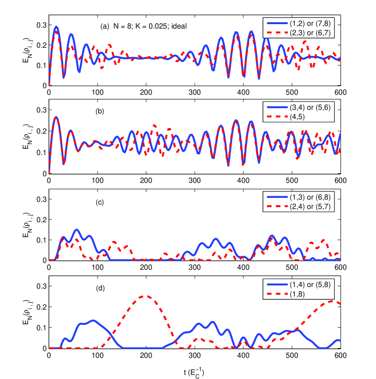
Figure 1: Pairwise entanglement creation for a homogeneous chain of $N=8$ qubits in ideal conditions; the system is described by the Hamiltonian of Equation (2) and the initial state is $|\Psi(0)\rangle$ of Equation (3). Note that symmetric qubit pairs, such as (1,2) and (7,8), generate the same entanglement and hence are represented by the same line. A ‘collapse-and-revival’ pattern emerges in the entanglement oscillations, as seen from a comparison of the different panels.

3 Influence of Disorder

In any experimental situation the initial preparation will also suffer from errors in the control parameters $\alpha_{\rm ctrl}=\epsilon_{i},\Delta_{i},K_{i}$. As a result, the homogeneity of the chain will be broken. We can simulate the effect by letting the parameters take random, but static, values in the interval $[(1-d)\alpha_{\rm ctrl},(1+d)\alpha_{\rm ctrl}]$, where $d$ quantifies the disorder. An example is shown in Figure 2(a), where we plot $E_{\rm N}(t)$ for the pair $(1,2)$ in the ideal (solid line) and imperfect scenario (broken line), where the disorder in $\Delta_{i}$ and $K_{i}$ is $d=0.05$. Averaging over $10^{4}$ runs, we have found that disorder with $d=0.01$, $d=0.05$, and $d=0.10$ causes relative fluctuations of the maximal entanglement equal to $0.011$, $0.027$ and $0.054$, respectively. Therefore for disorder which is less than $10\%$ (the upper bound in state-of-the-art experiments [29]) the entanglement in the system changes marginally, on average. This is indeed true for the noisy scenario also, as shown in the following section. It is noted that disorder has recently been studied in related, but different, contexts in [27, 30].

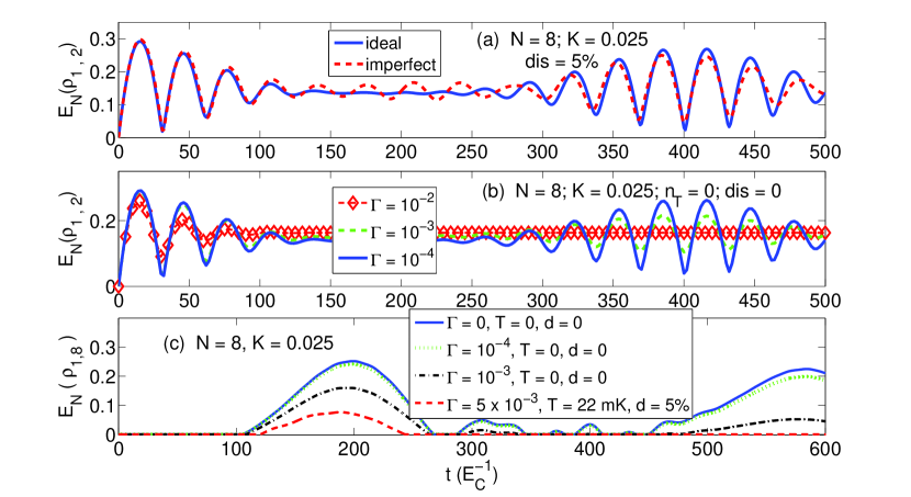
Figure 2: Entanglement creation between qubits $(1,2)$ in the presence of (a) disorder and (b) noise, which is characterised by a decay rate $\Gamma$ at absolute zero temperature. Subplot (c) shows $E_{N}(t)$ for qubits (1,8) for various values of the decay rate $\Gamma$, temperature, and disorder. In (a) the initial state is $|\Psi(0)\rangle$ of Equation (3) and it evolves under the Hamiltonian (2); in (b) and (c) the initial state is $|\psi(0)\rangle$ of Equation (8) and it evolves under the master equation (9).

4 Noise Model For a Variety of Sources

We consider a spin-boson Hamiltonian of the form

$${\cal H}_{\rm SB}={\cal H}_{\rm S}+{\cal H}_{\rm B}+\sum_{i=1}^{N}\sigma^{z}_{i}X_{i}$$ (5)

where the first term corresponds to the free system Hamiltonian of Equation (2), the second term is the Hamiltonian for all independent baths $i=\{1,2,\ldots,N\}$, ${\cal H}_{\rm B}=\sum_{i=1}^{N}\sum_{k}\Omega^{(i)}_{k}a^{(i)\dagger}_{k}a^{(i)}_{k}$, where the $k$-th mode of bath $i$ has boson creation and annihilation operators $a^{(i)\dagger}_{k}$ and $a^{(i)}_{k}$, respectively, and the third term is the interaction between a qubit and its bath, whose ‘force’ operator is $X_{i}=\sum_{l}{\cal G}^{(i)}_{l}\left[a_{l}^{(i)\dagger}+a^{(i)}_{l}\right]$ [17]. Clearly, it is assumed that each qubit is affected by its own bath, i.e., $[a^{(i)}_{k},a^{(j)\dagger}_{k}]=\delta_{ij}$, a reasonable requirement for charge qubits biased by independent voltage gates.

In the coherent regime, where $\omega_{i}\equiv(\epsilon_{i}^{2}+\Delta_{i}^{2})^{1/2}$ is much larger than the thermal energy, the preferred basis is given by the eigenstates of the single-qubit Hamiltonian, i.e., $\mbox{$|0\rangle$}=\cos(\theta_{i}/2)\mbox{$|\uparrow\rangle$}+\sin(\theta_{i}/2)\mbox{$|\downarrow\rangle$}$ and $\mbox{$|1\rangle$}=-\sin(\theta_{i}/2)\mbox{$|\uparrow\rangle$}+\cos(\theta_{i}/2)\mbox{$|\downarrow\rangle$}$, where the mixing angle obeys $\tan\theta_{i}=\Delta_{i}/\epsilon_{i}$. In this basis, ${\cal H}_{\rm SB}$ becomes

$${\cal H}^{\prime}_{\rm SB}={\cal H}^{\prime}_{\rm S}+{\cal H}_{\rm B}+\sum_{i=1}^{N}(\sin\theta_{i}\sigma^{x}_{i}+\cos\theta_{i}\sigma^{z}_{i})X_{i}$$ (6)

where

$${\cal H}^{\prime}_{\rm S}=-\frac{1}{2}\sum_{i=1}^{N}\omega_{i}\sigma^{z}_{i}-\frac{1}{2}\sum_{i=1}^{N-1}K_{i}(c_{i}\sigma^{z}_{i}+s_{i}\sigma^{x}_{i})(c_{i+1}\sigma^{z}_{i+1}+s_{i+1}\sigma^{x}_{i+1})$$ (7)

is the system Hamiltonian (the Pauli matrices are now written in the $\{\mbox{$|0\rangle$},\mbox{$|1\rangle$}\}$ basis) with $c_{i}=\cos\theta_{i},~{}s_{i}=\sin\theta_{i}$. In this basis the states $|\Psi(0)\rangle$ and $|\Phi(0)\rangle$ of Equations (3) and (4), respectively, become

$$|\psi(0)\rangle=\mbox{$|0\rangle$}^{\otimes N},\qquad|\phi(0)\rangle=\mbox{$|\beta^{\prime}\rangle$}_{12}\otimes\mbox{$|0\rangle$}^{\otimes N-2}$$ (8)

where $\mbox{$|\beta^{\prime}\rangle$}_{12}=2^{-1/2}(\mbox{$|01\rangle$}+\mbox{$|10\rangle$})$.

When the bath’s degrees of freedom are traced out, and within the Born-Markov approximation, the time evolution of the chain is governed by a master equation of the Lindblad form

$$\dot{\rho}=-i[H^{\prime}_{\rm S},\rho]+{\cal L}\rho$$ (9)

where $H^{\prime}_{\rm S}$ is given by the same expression of Equation (7) provided that the weak coupling limit, where $K_{i}<\omega_{i}$, holds. The damping terms are given by the usual expressions,

$${{\cal L}\rho=\sum_{i=1}^{N}[G_{i}(2\sigma_{i}^{+}\rho\sigma_{i}^{-}-\rho\sigma_{i}^{-}\sigma_{i}^{+}-\sigma_{i}^{-}\sigma_{i}^{+}\rho)+\tilde{G}_{i}(2\sigma_{i}^{-}\rho\sigma_{i}^{+}-\rho\sigma_{i}^{+}\sigma_{i}^{-}-\sigma_{i}^{+}\sigma_{i}^{-}\rho)}$$

$$+g_{i}(2\sigma_{i}^{z}\rho\sigma_{i}^{z}-2\rho)]$$ (10)

where $\sigma_{j}^{\pm}\equiv 2^{-1}(\sigma_{j}^{x}\pm i\sigma_{j}^{y})$ and the parameters are defined as

$$G_{i}=\sin^{2}\theta_{i}(1+n_{\rm T})\Gamma,\;\;\;\;\tilde{G}_{i}=\sin^{2}\theta_{i}n_{\rm T}\Gamma,\;\;\;\;g_{i}=\cos^{2}\theta_{i}\Gamma$$ (11)

with $n_{\rm T}$ denoting the average number of bosons in the environment. We assume that the environments of all qubits are identical. We have not specified the environment’s spectral properties and hence the decay rate $\Gamma$ is given as a phenomenological parameter whose exact value can be adjusted to match that obtained for the actual spectral density of the bath. Within this framework, a broad class of dissipative effects can be accounted for, ranging from electromagnetic fluctuations in the surrounding circuitry to, for instance, the coupling to a phonon bath [31]. The system can therefore be viewed as a non critical dissipative Ising chain (The critical behaviour of dissipative Ising chains has been recently addressed in [32].)

At the degeneracy point $\epsilon_{i}=0$ and $\cos\theta_{i}=0$. As a result, each qubit is susceptible to relaxation only (the ‘optimal’ point introduced in Reference [7]). If, however, the energy bias is not exactly zero then the longitudinal contribution $\sigma^{z}_{i}X_{i}$ leads to pure dephasing at a rate $g_{i}$. In any experimental realization, the presence of disorder limits the accuracy with which qubits can be operated at their optimal points, especially when it comes to the operation of long chains. In what follows we take this into account and study the modifications due to disorder. In current experiments [29] the value of disorder is typically $5-10\%$ at temperatures $20-40~{}m{\rm K}$. The decoherence time $t_{\rm d}\equiv\Gamma^{-1}$ for two coupled charged qubits [10] was reported to be around $2.5~{}n{\rm s}$ (for single qubits $t_{\rm d}$ can be higher). In our simulations below we usually assume a worst-case scenario and let $d=5\%$ at $T\approx 41~{}m{\rm K}$ with decay rate $\Gamma=10^{-2}E_{C}$ (which corresponds to $t_{\rm d}\approx 1~{}n{\rm s}$).

5 Dynamics of Short Chains $(N\sim 10$ qubits)

In this section we discuss the results on the entanglement dynamics of open chains with $N=8$ qubits (Figures 1-6). Figures 1 and 2(a) have been analysed previously. Figure 2(b) shows the creation of entanglement in the pair $(1,2)$ for various values of the relaxation rate $\Gamma$. Figure 2(c) shows the creation of entanglement in the pair $(1,8)$ for various values of $\Gamma$ and other parameters. It is seen that for noise strength $\Gamma=5\times 10^{-3}$ (i.e., $t_{\rm d}\approx 5~{}n{\rm s}$), average number of photons $n_{\rm T}=0.01$ (i.e., $T\approx 22~{}m{\rm K}$) and disorder $d=5\%$ one may still obtain substantial entanglement between the first and last qubit in the chain (in particular, the ratio of the values of the first maxima corresponding to the imperfect / ideal cases is approximately $2/5$).

In Figure 3 we plot $E_{N}(t)$ for different pairs of qubits in the case of (top) relaxation with $\Gamma=10^{-2}$ at zero temperature ($T=0$) and (bottom) relaxation with $\Gamma=10^{-2}$, finite temperature $T\approx 41~{}m{\rm K}$ ($n_{\rm T}=0.1$) or $T\approx 33~{}m{\rm K}$ ($n_{\rm T}=0.05$), and disorder $5\%$ ($d=0.05$). As expected, the entanglement beyond nearest neighbours is drastically reduced in the presence of larger values of the noise (the correlations between the first and last qubit in the chain vanish altogether for this high value of $\Gamma$).

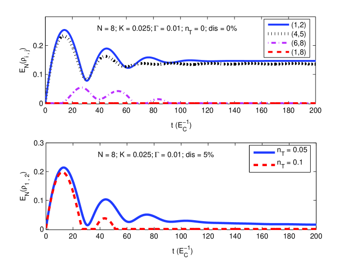
Figure 3: Entanglement creation between two qubits for the case of relaxation only (top) and relaxation, finite temperature, and disorder (bottom). The initial state is $|\psi(0)\rangle$ of Equation (8) and the system evolves under the master equation (9).

In Figure 4 we study the creation of entanglement between the first two qubits in the chain (in subplots (a) and (b)) when the initial state is the ground state of the Hamiltonian ${\cal H}^{\prime}_{\rm S}(K_{\rm ini})$ of Equation (7), for various values of the initial coupling strength $K_{\rm ini}$. At $t=0$ the coupling is instantaneously switched on to its final value $K_{\rm fin}=\Delta/4$. Subplot (a) shows the case with noise, at absolute zero temperature. Subplot (b) takes into account the temperature in the environment ($T\approx 41~{}m{\rm K}$). In subplot (c) we study the case whereby at $t=0$ the state of the system is in thermal equilibrium with its environment at temperature $T_{0}$. Therefore in this case we let $\rho(T_{0})=\exp(-\beta{\cal H}^{\prime}_{\rm S})/Z$ at $t=0$. The system Hamiltonian ${\cal H}^{\prime}_{\rm S}$, given by Equation (7), depends on the initial interqubit coupling $K_{\rm ini}$. The evolution proceeds according to the master equation (9) with the coupling $K_{\rm fin}$ and an average number of photons $n_{\rm T}$ that corresponds to the temperature $T_{0}$. It is seen that at operating temperatures of around $40~{}m{\rm K}$ the entanglement vanishes. It is however possible to observe entanglement when the temperature gets smaller (e.g., for $T_{0}\approx 33~{}m{\rm K}$).

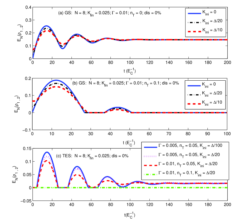
Figure 4: Entanglement creation between qubits (1,2) in noisy conditions when there is some initial homogeneous coupling $K_{\rm ini}$ that is instantaneously switched on to $K_{\rm fin}=\Delta/4$ at $t=0$. In subplots (a) and (b) the initial state is the ground state (‘GS’) of ${\cal H}^{\prime}_{\rm S}(K_{\rm ini})$ of Equation (7) and they correspond to temperatures $T=0$ and $T\approx 41~{}m{\rm K}$ ($n_{\rm T}=0.1$). In subplot (c) the initial state is the thermal equilibrium state (‘TES’) of the system at a given temperature $T$, for various values of the parameters.

The results in Figure 4 seem to indicate that the increase in the noise strength $\Gamma$ and the external temperature yield the unavoidable degrading of entanglement generation. The amplitude of the entanglement oscillations decreases and the system becomes separable in the steady state for $\Gamma$ and/or $n_{\rm T}$ sufficiently large. However, this behaviour is not universal and we need to differentiate two time scales in the system. The initial transient is always such that the amplitude of entanglement oscillations is reduced as the noise increases and the amplitude of the first entanglement maximum is a monotonically decreasing function of both $\Gamma$ and $T$. However, for a fixed $n_{\rm T}$, the steady-state entanglement can display a non-monotonic behaviour as a function of $\Gamma$. This phenomenon is of the same type of the noise-assisted effects that have been studied in Reference [33] for weakly driven spin chains and is illustrated in Figure 5 for a system of $N=4$ qubits. We see that at the selected temperature where $n_{\rm T}=0.1$, there are parameter regimes for which the steady-state entanglement is initially zero for low values of the noise strength and resurfaces when $\Gamma$ is increased over a certain threshold. This result indicates that if the aim is to generate entanglement in the steady state, it may be advantageous to amplify the environmental noise so as to maximise entanglement production along the chain. Persistence of this effect in longer chains $(N\sim 40$) has been corroborated numerically.

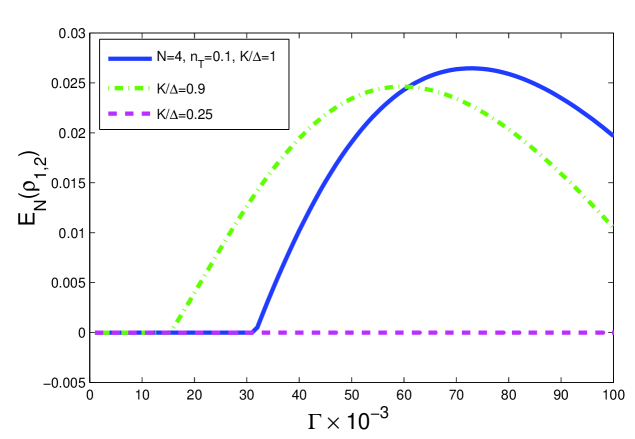
Figure 5: Steady state entanglement between qubits (1,2) in a chain of $N=4$ when $n_{\rm T}=0.1$ and for different values of the ratio $K/\Delta$ as a function of the noise strength $\Gamma$. Parameter regimes can be identified where entanglement generation is enhanced by amplifying the environmental noise.

Propagation of entanglement is analysed in Figure 6 for (a) ideal and (b) non-ideal conditions. In the ideal case, entanglement propagates from the first two qubits to the last two, but not perfectly. When we take into account noise and disorder the entanglement transfer is not possible and the last two qubits quickly reach their steady state, which is slightly entangled at absolute zero temperature, but separable at $T\sim 20~{}m{\rm K}$ for the selected parameter regime.

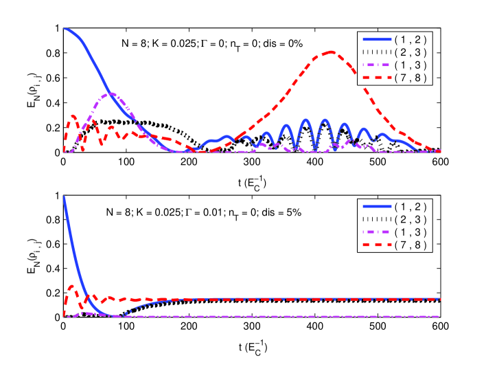
Figure 6: Entanglement propagation at zero temperature for the ideal case (top) and for relaxation and disorder (bottom). In the top plot, the initial state is $|\Psi(0)\rangle$ of Equation (4) and the system is described by the Hamiltonian ${\cal H}_{\rm S}$ of Equation (2). In the bottom plot the initial state is $|\phi(0)\rangle$ of Equation (8) and it evolves under the master equation (9).

6 Dynamics of Long Chains

To confirm the validity of our findings for longer chains, we have performed time-dependent DMRG simulations [20].

For an ideal chain without noise and disorder, we have considered entanglement generation in the model (2) with $N=20$ qubits. Here the matrix dimension was chosen $dim=20$ and a 4th order Suzuki-Trotter decomposition was employed. The results are in good agreement with the findings for shorter chains in figure 1. In particular, we observe the same ‘collapse-and-revival’ pattern of the entanglement oscillations, and the long-range entanglement peaks at those regions where the short-range entanglement is close to its steady-state value or vanishes altogether.

For the cases which include noise and disorder, a matrix product representation for mixed states with matrix dimension $dim=60$ and a 4th order Suzuki-Trotter decomposition were used for a chain of $N=40$ qubits [20]. A sketch of the method is given in A.

Figure 7 shows the creation of entanglement in the presence of noise, at zero temperature for both a homogeneous and a disordered chain (in which case disorder occurs in $\epsilon_{i}$ as well as $\Delta_{i},K_{i}$). Figure 8 shows entanglement creation in a noisy homogeneous chain for various values of temperature. For all quantities we find good agreement with the results obtained for $N=8$, where the relative deviations between $N=40$ and $N=8$ are less than $5\%$. It is also noted that the entanglement between two blocks of two qubits each was found to be about $17\%$ higher than the entanglement between individual qubits of the same separation.

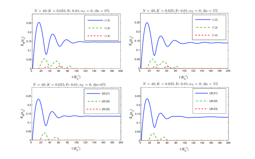
Figure 7: Entanglement creation, i.e. evolution of the initial state $|\psi(0)\rangle$, (8), given by Equation (9) in a chain of $N=40$ qubits at zero temperature, in the presence of noise ($\Gamma=0.01$). The two plots on the left show the homogeneous case, while the two plots on the right show a case with $5\%$ disorder in $\epsilon_{i},\Delta_{i},K_{i}$. Qubits at the boundaries are slightly stronger entangled than in the centre of the chain. The entanglement between qubits that are further apart than shown here is zero.

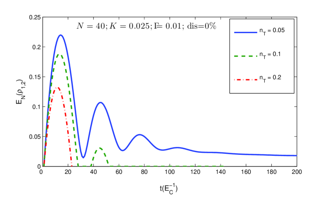
Figure 8: Entanglement creation, i.e. evolution of the initial state $|\psi(0)\rangle$, (8), given by equation (9) in a chain of $N=40$ qubits at various temperatures ($n_{\rm T}=0.05;n_{\rm T}=0.1$ and $n_{\rm T}=0.2$) in the presence of noise ($\Gamma=0.01$). Only nearest neighbours become entangled in this case.

7 Witnessing Quantum Correlations: Experimental Verification of Entanglement

In experiments it will be crucial to verify the existence of entanglement via measurements, which ideally should also permit a quantification of the detected entanglement. This could be done by full state tomography, which is a very costly experimental procedure though. Being able to establish a lower bound on entanglement from the measurement of a few observables will thus be a significant advantage. Recently, a theoretical framework for the exploration of these questions has been developed for general observables [26] and witness operators [34].

The basic approach is to identify the least entangled quantum state that is compatible with the measurement data. The entanglement of that state then provides a quantitative value for the entanglement that can be guaranteed given the measurement data. In [26], in particular, spin-spin correlations have been used to determine such a lower bound analytically. We now employ this concept for our system and consider the two quantities,

$$C_{1}(\rho_{i,j}) \equiv {\rm max}\left[0,\log_{2}\left(|C^{xx}_{i,j}|+|C^{zz}_{i,j}|\right)\right]$$ (12)

$$C_{2}(\rho_{i,j}) \equiv {\rm max}\left[0,\log_{2}\left(1+|C^{xx}_{i,j}|+|C^{yy}_{i,j}|+|C^{zz}_{i,j}|\right)-1\right]$$ (13)

where $C^{ab}_{i,j}={\rm Tr}[\sigma_{i}^{a}\sigma_{j}^{b}\rho]$ ($a,b=x,y,z$). Both quantities form a lower bound to the logarithmic negativity, i.e. $E_{\rm N}(\rho_{i,j})\geq C_{1}(\rho_{i,j})$ and $E_{\rm N}(\rho_{i,j})\geq C_{2}(\rho_{i,j})$. $C_{1}(\rho_{i,j})$ can be employed if only $C^{xx}_{i,j}$ and $C^{zz}_{i,j}$ are accessible in measurements. However, if $C^{yy}_{i,j}$ can be measured too, then $C_{2}(\rho_{i,j})$ yields a tighter bound.

Figure 9 shows that both lower bounds provide good approximations for the logarithmic negativity of two neighbouring qubits. If the qubits are next-nearest neighbours, $C_{2}(\rho_{i,j})$ still provides a good estimate, while $C_{1}(\rho_{i,j})$ eventually fails to approximate the entanglement well.

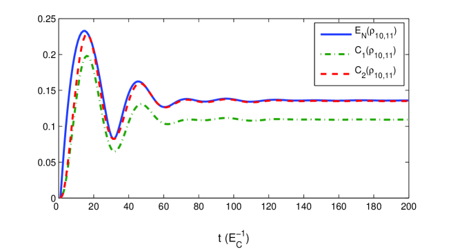
Figure 9: The logarithmic negativity (1) and the two lower bounds (12) for a chain of $N=40$ qubits with $\Delta=0.1$, $K=0.025$ and $\Gamma=0.01$ at $n_{\rm T}=0$.

The reason why $C_{1}(\rho_{i,j})$ and $C_{2}(\rho_{i,j})$ sometimes do not approximate the entanglement very well lies in the choices of the axes along which correlations are measured. Instead of $C^{xx}_{i,j}$, $C^{yy}_{i,j}$ and $C^{zz}_{i,j}$ one could consider correlations along a rotated set of axes, $C^{aa}_{i,j}$, $C^{bb}_{i,j}$ and $C^{cc}_{i,j}$, where $\sigma_{i}^{a}=\sum_{\alpha=x,y,z}R_{a\alpha}\sigma_{i}^{\alpha}$ and $R_{a\alpha}$ is an orthogonal matrix representing the rotation. Choosing to measure correlations along $x$, $y$ and $z$ may hence underestimate the entanglement severely. The best approximation of the entanglement is obtained by maximising $C^{aa}_{i,j}$, $C^{bb}_{i,j}$ and $C^{cc}_{i,j}$ over all possible choices for the axes $a$, $b$ and $c$.

This optimal choice can be obtained in the following way: If the state $\rho$ is symmetric with respect to subsystems $i$ and $j$ in the sense that $C^{xy}_{i,j}=C^{yx}_{i,j}$, $C^{xz}_{i,j}=C^{zx}_{i,j}$ and $C^{yz}_{i,j}=C^{zy}_{i,j}$, then the matrix

$$X=\left(\begin{array}[]{ccc}C^{xx}_{i,j}&C^{xy}_{i,j}&C^{xz}_{i,j}\\ C^{yx}_{i,j}&C^{yy}_{i,j}&C^{yz}_{i,j}\\ C^{zx}_{i,j}&C^{zy}_{i,j}&C^{zz}_{i,j}\end{array}\right)$$ (14)

is real and symmetric and hence has real eigenvalues and is diagonalised by a rotation. Let us denote the eigenvalues of $X$ by $\lambda_{1}$, $\lambda_{2}$ and $\lambda_{3}$, then the quantity

$$C^{\prime}_{2}(\rho_{i,j})\equiv{\rm max}\left[0,\log_{2}\left(1+|\lambda_{1}|+|\lambda_{2}|+|\lambda_{3}|\right)-1\right]$$ (15)

provides the best approximation of $E_{\rm N}(\rho_{i,j})$ of the form (12), as $\lambda_{1}$, $\lambda_{2}$ and $\lambda_{3}$ are the spin-spin correlations along the optimal choice of axes .

As an example, in figure 9, the entanglement between qubits 10 and 11 is $E_{\rm N}(\rho_{10,11})=0.2096$ at $t=10E_{C}^{-1}$. While $C_{2}(\rho_{10,11})=0.1583$ at this point, we obtained $C^{\prime}_{2}(\rho_{10,11})=0.2096$ for the optimal choice of axes $a$, $b$ and $c$. The optimal choice of axes depends on time. Yet one fixed set of axes approximated the entanglement very well over a range of $\Delta t=5E_{C}^{-1}$ in our example.

8 Conclusions

We have studied the dynamics of entanglement in qubit chains influenced by noise and static disorder. This study provides useful analysis for interesting experiments with quantum devices that in the long term may be suitable for the implementation of quantum computing. We have considered an experimentally interesting implementation using Josephson charge qubits with capacitive interactions between nearest neighbours. We have found that static disorder less than $10\%$ (i.e., the current experimental upper bound) does not affect the entanglement dynamics substantially. By contrast, the influence of environmental noise, modelled here as a set of independent harmonic oscillator baths of arbitrary spectral density, is much more pronounced: it reduces long-range correlations and decreases the magnitude of the achievable bipartite entanglement. For typical operating temperatures, the influence of noise on the chain dynamics at short times and in the steady-state can be crucially distinct; while the entanglement amplitudes in the initial transient decrease monotonically with the noise strength, the steady-state response is non-monotonic. Therefore, we have identified parameter regimes in which the bipartite entanglement increases as a result of amplifying the noise. We have found agreement between the behaviour of entanglement in short ($N\sim 10$) and long ($N\sim 50$) chains.

The present results are encouraging from the experimental point of view as they suggest that (a) both short- and long-range entanglement can be generated and propagated under suitable laboratory conditions, and (b) lower bounds can be placed on the entanglement from the measurement of a few general observables.

Appendix A Matrix Product State Simulations for Mixed States

Here we outline the concept proposed in [20] and its adaption to our application. For the Matrix Product State simulation of mixed state dynamics, the density matrix for $N$ qubits is expanded in a basis of matrices formed by direct products of the elementary matrices

$$\epsilon_{1}=\left(\begin{array}[]{cc}1&0\\ 0&0\end{array}\right);\quad\epsilon_{2}=\left(\begin{array}[]{cc}0&1\\ 0&0\end{array}\right);$$ (20)

$$\epsilon_{3}=\left(\begin{array}[]{cc}0&0\\ 1&0\end{array}\right);\quad\epsilon_{4}=\left(\begin{array}[]{cc}0&0\\ 0&1\end{array}\right).$$ (25)

Hence the matrices forming the basis for $N$ qubits are of the form

$$\underbrace{\epsilon_{i}\otimes\epsilon_{j}\otimes\dots\otimes\epsilon_{l}}_{N~{}{\rm sites}}.$$ (26)

The expansion of the density matrix $\rho$ is now written in terms of products of matrices in the following way:

$$\rho=\sum_{s_{1},s_{2},\dots s_{N}=1}^{4}\,\Gamma_{1}^{[s_{1}]}\cdot\Lambda_{1}\cdot\Gamma_{2}^{[s_{2}]}\cdot\Lambda_{2}\cdot\dots\cdot\Lambda_{N-1}\cdot\Gamma_{N}^{[s_{N}]}\>\epsilon_{s_{1}}\otimes\epsilon_{s_{2}}\otimes\dots\otimes\epsilon_{s_{N}}$$ (27)

where ‘$\cdot$’ denotes matrix multiplication. Here, each $\Gamma_{1}^{[s_{1}]}$ ($s_{1}=1,2,3,4$) is a row vector of length $D$, each $\Gamma_{N}^{[s_{N}]}$ is a column vector of length $D$, each $\Gamma_{j}^{[s_{j}]}$ ($j\not=1,N$) is a $D\times D$ matrix and each $\Lambda_{j}$ is a diagonal $D\times D$ matrix. The structure of the matrices $\Gamma$ and $\Lambda$ is the same as in the Matrix Product representation of pure states and the TEBD-algorithm [20] can be employed for the simulation of the dynamics. In contrast to pure states, the matrix elements of the $\Lambda_{j}$ for mixed states can however no longer be interpreted as the Schmidt coefficients of the respective decomposition.

References

References

-
[1]
A.J. Leggett and A. Garg, Phys. Rev. Lett. 54, 857
(1985).
A.J. Leggett, J. Phys.: Condens. Matter 14, R415 (2002). - [2] A.N. Jordan, A.N. Korotkov, M. Büttiker, Phys. Rev. Lett. 97, 026805 (2006).
-
[3]
Y. Makhlin, G. Schön, A. Shnirman, Rev. Mod. Phys.
73, 357 (2001).
M.H. Devoret, A. Wallraff, J.M. Martinis, cond-mat/0411174.
J. Q. You and F. Nori, Phys. Today 58, 42 (2005). - [4] Y. Nakamura, Y.A. Pashkin, J.S. Tsai, Nature 398, 786 (1999).
- [5] J.E. Mooij, T.P. Orlando, L. Levitov, L. Tian, C.H. van der Wal, S. Lloyd, Science 285, 1036 (1999).
- [6] J.Q. You, J.S. Tsai, F. Nori, Phys. Rev. Lett. 89, 197902 (2002).
- [7] D. Vion, A. Aassime, A. Cottet, P. Joyez, H. Pothier, C. Urbina, D. Esteve, M.H. Devoret, Science 296, 886 (2002).
- [8] Y. Yu, S. Han, X. Chu, S-I Chu, Z. Wang, Science 296, 889 (2002).
- [9] M. Wallquist, J. Lantz, V.S. Shumeiko, G. Wendin, New J. Phys. 7, 178 (2005).
-
[10]
Y.A. Pashkin, T. Yamamoto, O. Astafiev, Y. Nakamura, D.V. Averin,
J.S. Tsai, Nature 421, 823 (2003).
T. Yamamoto, Y.A. Pashkin, O. Astaviev, Y. Nakamura, J.S. Tsai, Nature 425, 941 (2003). -
[11]
J.B. Majer, F.G. Paauw, A.C.J. ter Haar, C.J.P.M. Harmans, J.E.
Mooij, Phys. Rev. Lett. 94, 090501 (2005).
R. McDermott, R.W. Simmonds, M. Steffen, K.B. Cooper, K. Cicak, K.D. Osborn, S. Oh, D.P. Pappas, J.M. Martinis , Science 307, 1299 (2005). -
[12]
M. Paternostro, G.M. Palma, M.S. Kim, G. Falci, Phys. Rev. A
71, 042311 (2005).
P. Rabl, D. DeMille, J.M. Doyle, M.D. Lukin, R.J. Schoelkopf, P. Zoller , Phys. Rev. Lett. 97, 033003 (2006). -
[13]
A. Romito, R. Fazio, C. Bruder, Phys. Rev. B 71,
100501(R) (2005).
A. Lyakhov and C. Bruder, New J. Phys. 7, 181 (2005). - [14] S. Bose, Phys. Rev. Lett. 91, 207901 (2003).
- [15] J.E. Mooij, private communication (2005).
-
[16]
D. Loss and K. Mullen, Phys. Rev. A 43, 2129 (1991).
P. Cedraschi and M. Büttiker, Phys. Rev. B 63, 165312 (2001).
J.P. Pekola and J.J. Toppari, Phys. Rev. B 64, 172509 (2001).
E. Almaas and D. Stroud, Phys. Rev. B 65, 134502 (2002).
H. Kohler, F. Guinea, F. Sols, Ann. Phys. 31, 127 (2004). - [17] See A. Shnirman, Y. Makhlin, G. Schön, Phys. Scr. T102, 147 (2002) and references therein.
-
[18]
Y. Nakamura, Y.A. Pashkin, T. Yamamoto, J.S. Tsai, Phys. Rev.
Lett. 88, 047901 (2002).
E. Paladino, L. Faoro, G. Falci, R. Fazio, ibid. 88, 228304 (2002).
O. Astafiev, Y.A. Pashkin, Y. Nakamura, T. Yamamoto, J.S. Tsai, ibid. 93, 267007 (2004).
L. Faoro, J. Bergli, B.L. Altshuler, Y.M. Galperin, ibid. 95, 046805 (2005).
A. Shnirman, G. Schön, I. Martin and Y. Makhlin, ibid. 94, 127002 (2005).
J. Schriefl, Y. Makhlin, A. Shnirman and G. Schön, New J. Phys. 8, 1 (2006). -
[19]
M.J. Storcz and F.K. Wilhelm, Phys. Rev. A 67, 042319
(2003).
J.Q. You, X. Hu, F. Nori, Phys. Rev. B 72, 144529 (2005).
B. Ischi, M. Hilke, M. Dubé, Phys. Rev. B 71, 195325 (2005). -
[20]
G. Vidal, Phys. Rev. Lett. 93, 040502 (2004).
M. Zwolak and G. Vidal, Phys. Rev. Lett. 93, 207205 (2004). - [21] M.J. Hartmann, M.E. Reuter, M.B. Plenio, New. J. Phys. 8, 94 (2006).
- [22] M.B. Plenio and S. Virmani, Quant. Inf. Comp. 7, 1 (2007).
-
[23]
J. Eisert, PhD thesis, University of Potsdam (2001).
M.B. Plenio, Phys. Rev. Lett. 95, 090503 (2005). - [24] K. Audenaert, M.B. Plenio and J. Eisert, Phys. Rev. Lett. 90, 027901 (2003)
- [25] M. Steffen, M. Ansmann, R.C. Bialczak, N. Katz, E. Lucero, R. McDermott, M. Neeley, E.M. Weig, A.N. Cleland, J.M. Martinis, Science 313, 1423 (2006).
- [26] K. Audenaert and M.B. Plenio, New J. Phys. 8, 266 (2006).
- [27] J. Eisert, M.B. Plenio, S. Bose, J. Hartley, Phys. Rev. Lett. 93, 190402 (2004).
- [28] M.B. Plenio, J. Hartley, J. Eisert, New J. Phys. 6, 36 (2004)
- [29] P. Meeson, private communication (2006).
-
[30]
S. Montangero and L. Viola, Phys. Rev. A 73, 040302(R)
(2006).
S. Montangero, G. Benenti, R. Fazio, Phys. Rev. Lett. 91, 187901 (2003). - [31] L.B. Ioffe, V.B. Geshkenbein, Ch. Helm, G. Blatter, Phys. Rev. Lett. 93, 057001 (2004).
- [32] P. Werner, K. Völker, M. Troyer, S. Chakravarty, Phys. Rev. Lett. 94, 047201 (2005).
- [33] S.F. Huelga and M.B. Plenio, quant-ph/0608164.
-
[34]
J. Eisert, F.G.S.L. Brandão, K. Audenaert, quant-ph/0607167.
O. Gühne, M. Reimpell, R.F. Werner, quant-ph/0607163. - [35] R. Bhatia, Matrix Analysis, (Springer-Verlag, New York, 1997).