Breakdown of the few-level approximation in collective systems

Abstract

The validity of the few-level approximation in dipole-dipole interacting collective systems is discussed. As example system, we study the archetype case of two dipole-dipole interacting atoms, each modelled by two complete sets of angular momentum multiplets. We establish the breakdown of the few-level approximation by first proving the intuitive result that the dipole-dipole induced energy shifts between collective two-atom states depend on the length of the vector connecting the atoms, but not on its orientation, if complete and degenerate multiplets are considered. A careful analysis of our findings reveals that the simplification of the atomic level scheme by artificially omitting Zeeman sublevels in a few-level approximation generally leads to incorrect predictions. We find that this breakdown can be traced back to the dipole-dipole coupling of transitions with orthogonal dipole moments. Our interpretation enables us to identify special geometries in which partial few-level approximations to two- or three-level systems are valid.

I Introduction

The theoretical analysis of any non-trivial physical problem typically requires the use of approximations. A key approximation facilitated in most areas of physics reduces the complete configuration space of the system of interest to a smaller set of relevant system states. In the theoretical description of atom-field interactions, the essential state approximation entails neglecting most of the bound and continuum atomic states Scully and Zubairy (1997); Ficek and Swain (2005); aga . The seminal Jaynes-Cummings-Model Jaynes and Cummings (1963) takes this reduction to the extreme in that only two atomic states are retained. Obviously, it is essential to in detail explore the validity range of this reduction of the configuration space. The few-level approximation usually leads to theoretical predictions that are well verified experimentally Scully and Zubairy (1997); Ficek and Swain (2005), and is generally considered as understood for single-atom systems. It fails, however, to reproduce results of quantum electrodynamics, where in general all possible intermediate atomic states need to be considered in order to obtain quantitatively correct results Lamb et al. (1987). The situation becomes even less clear in collective systems, where the individual constituents interact via the dipole-dipole interaction, despite the relevance of collectivity to many areas of physics. Examples for such systems can be found in ultracold quantum gases Thirunamachandran (1980), trapped atoms DeVoe and Brewer (1996); Kästel and Fleischhauer (2005), or solid state systems Hettich et al. (2002); Barnes et al. (2005), with applications, e.g., in quantum information theory Lukin and Hemmer (2000).

Therefore, we discuss the validity of the few-level approximation in dipole-dipole interacting collective systems. For this, we study the archetype case of two dipole-dipole interacting atoms, see Fig. 1(a). Experiments of this type have become possible recently DeVoe and Brewer (1996); Hettich et al. (2002). In order to remain general, each atom is modelled by complete sets of angular momentum multiplets, as shown in Fig. 1(b). We find that the few-level approximation in general leads to incorrect predictions if it is applied to the magnetic sublevels of this system. For this, we first establish a general statement about the system behavior under rotations of the atomic separation vector $\boldsymbol{R}$. As a first conclusion from this result, we derive the intuitive outcome that the dipole-dipole induced energy shifts between collective two-atom states are invariant under rotations of the separation vector $\boldsymbol{R}$. This result can only be established if complete and degenerate multiplets are considered and dipole-dipole interactions between orthogonal transition dipole moments are included in the analysis. On the contrary, the artificial omission of any of the Zeeman sublevels of a multiplet leads to a spurious dependence of the energy shifts on the orientation, and thus to incorrect predictions.

For example, if in the well-known two-level approximation only one excited state $|e\rangle$ and the ground state $|g\rangle$ are retained, then we recover the position-dependent energy splitting between the entangled two-particle states $(|e,g\rangle\pm|g,e\rangle)/\sqrt{2}$ that has previously been reported for a pair of two-level systems aga ; Ficek and Swain (2005). This geometry-dependence is at odds with the rotational invariance of the collective energy splitting expected for the degenerate system with all Zeeman sublevels. We thus conclude that the few-level approximation in general cannot be applied to this system.

Our results can be generalized to more complex angular momentum multiplets.

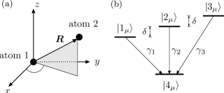
Figure 1: (a) The system of interest is comprised of two identical atoms that are located at $\boldsymbol{r}_{1}$ and $\boldsymbol{r}_{2}$, respectively. $\boldsymbol{R}=\boldsymbol{r}_{2}-\boldsymbol{r}_{1}$ is the relative position of atom 2 with respect to atom 1. (b) Level structure of atom $\mu\in\{1,2\}$ which we employ to illustrate our results. The ground state is a $S_{0}$ singlet state, and the three excited levels are Zeeman sublevels of a $P_{1}$ triplet. $\delta$ is the frequency splitting of the upper levels.

II The Model

We describe each atom by a $S_{0}\leftrightarrow P_{1}$ transition shown in Fig. 1(b) that can be found, e.g., in ⁴⁰Ca atoms. We choose the $z$ axis as the quantization axis, which is distinguished by an external magnetic field that induces a Zeeman splitting $\delta$ of the excited states. The orientation of $\boldsymbol{R}$ is defined relative to this quantization axis. We begin with the introduction of the master equation which governs the atomic evolution of the system shown in Fig. 1. The internal state $|i_{\mu}\rangle$ of atom $\mu$ is an eigenstate of $J_{z}^{(\mu)}$, where $\boldsymbol{J}^{(\mu)}$ is the angular momentum operator of atom $\mu$ ($\mu\in\{1,2\}$). In particular, the $P_{1}$ multiplet with $J=1$ corresponds to the excited states $|1_{\mu}\rangle$, $|2_{\mu}\rangle$ and $|3_{\mu}\rangle$ with magnetic quantum numbers $m=-1,\,0$ and 1, respectively, and the $S_{0}$ state is the ground state $|4_{\mu}\rangle$ with $J=m=0$. The raising and lowering operators on the $|4_{\mu}\rangle\leftrightarrow|i_{\mu}\rangle$ transition of atom $\mu$ are ($i\in\{1,2,3\}$)

$$S_{i\,+}^{(\mu)}=|i_{\mu}\rangle\langle 4_{\mu}|\quad\text{and}\quad S_{i\,-}^{(\mu)}=|4_{\mu}\rangle\langle i_{\mu}|\,.$$ (1)

The total system Hamiltonian for the two atoms and the radiation field is $H=H_{\text{A}}+H_{\text{F}}+V\,,$ where

$$H_{\text{A}}= \hbar\sum\limits_{i=1}^{3}\sum\limits_{\mu=1}^{2}\omega_{i}\,S_{i\,+}^{(\mu)}S_{i\,-}^{(\mu)}\,,\quad H_{\text{F}}=\sum\limits_{\boldsymbol{k}s}\hbar\omega_{k}a_{\boldsymbol{k}s}^{\dagger}a_{\boldsymbol{k}s}\,,$$

$$V= -\boldsymbol{\hat{d}}^{(1)}\cdot\boldsymbol{\hat{E}}(\boldsymbol{r}_{1})-\boldsymbol{\hat{d}}^{(2)}\cdot\boldsymbol{\hat{E}}(\boldsymbol{r}_{2})\,.$$ (2)

In these equations, $H_{\text{A}}$ describes the free evolution of the two identical atoms, $\hbar\omega_{i}$ is the energy of state $|i_{\mu}\rangle$ and we choose $\hbar\omega_{4}=0$. $H_{\text{F}}$ is the Hamiltonian of the vacuum field and $V$ describes the interaction of the atoms with the vacuum modes in dipole approximation. The electric field operator $\boldsymbol{\hat{E}}$ is defined as

$$\boldsymbol{\hat{E}}(\boldsymbol{r})=i\sum\limits_{\boldsymbol{k}s}\sqrt{\frac{\hbar\omega_{k}}{2\varepsilon_{0}v}}\boldsymbol{\epsilon}_{\boldsymbol{k}s}e^{i\boldsymbol{k}\cdot\boldsymbol{r}}a_{\boldsymbol{k}s}+\text{H.c.}\,,$$ (3)

where $a_{\boldsymbol{k}s}$ ($a_{\boldsymbol{k}s}^{\dagger}$) are the annihilation (creation) operators that correspond to a field mode with wave vector $\boldsymbol{k}$, polarization $\boldsymbol{\epsilon}_{\boldsymbol{k}s}$ and frequency $\omega_{k}$, and $v$ denotes the quantization volume. The electric-dipole moment operator of atom $\mu$ is a vector operator with respect to the angular momentum operator $\boldsymbol{J}^{(\mu)}$ of atom $\mu$ and reads

$$\boldsymbol{\hat{d}}^{(\mu)}=\sum\limits_{i=1}^{3}\big{[}\boldsymbol{d}_{i}S_{i\,+}^{(\mu)}+\text{H.c.}\big{]}\,.$$ (4)

We determine the dipole moments $\boldsymbol{d}_{i}=\langle i|\boldsymbol{\hat{d}}|4\rangle$ via the Wigner-Eckart theorem Sakurai (1994) and find

$$\boldsymbol{d}_{1} =\mathcal{D}\,\boldsymbol{\epsilon}^{(+)}\,,\qquad\boldsymbol{d}_{3}=-\mathcal{D}\,\boldsymbol{\epsilon}^{(-)}\,,$$ (5a)

$$\boldsymbol{d}_{2} =\mathcal{D}\,\boldsymbol{e}_{z}\,,$$ (5b)

where $\mathcal{D}$ is the reduced dipole matrix element and the circular polarization vectors are $\boldsymbol{\epsilon}^{(\pm)}=(\boldsymbol{e}_{x}\pm i\boldsymbol{e}_{y})/\sqrt{2}$.

We now adapt the standard derivation of a master equation Scully and Zubairy (1997); Ficek and Swain (2005); aga to our multilevel system. For this, we assume that the radiation field is initially in the vacuum state denoted by $\varrho_{\text{F}}$ and suppose that the total density operator factorizes into a product of $\varrho_{\text{F}}$ and the atomic density operator $\varrho$ at $t=0$. The master equation for the reduced atomic density operator in Born approximation then takes the form

$$\partial_{t}\varrho= -\frac{i}{\hbar}[H_{\text{A}},\varrho]$$ (6)

$$-\frac{1}{\hbar^{2}}\int\limits_{0}^{t}d\tau\text{Tr}_{\text{F}}\Big{(}\big{[}V,U(\tau)\big{[}V,\varrho_{\text{F}}\varrho(t-\tau)\big{]}U^{\dagger}(\tau)\big{]}\Big{)}\,,$$

where $U(\tau)=\exp[-i(H_{\text{A}}+H_{\text{F}})\tau/\hbar]$ and $\text{Tr}_{\text{F}}()$ denotes the trace over the vacuum modes. We evaluate the integral in Eq. (6) in Markov-approximation Scully and Zubairy (1997) and ignore all terms associated with the Lamb shift of the atomic levels. In addition, we employ the rotating-wave approximation and neglect anti-resonant terms that are proportional to $S_{i\,+}^{(\mu)}S_{j\,+}^{(\nu)}$ and $S_{i\,-}^{(\mu)}S_{j\,-}^{(\nu)}$. We finally obtain

$$\partial_{t}\varrho=-\frac{i}{\hbar}[H_{\text{A}},\varrho]-\frac{i}{\hbar}[H_{\Omega},\varrho]+\mathcal{L}_{\gamma}\varrho\,.$$ (7)

In this equation, the Hamiltonian $H_{\Omega}$ describes the coherent part of the dipole-dipole interaction and reads

$$H_{\Omega}=-\hbar\sum\limits_{i,j=1}^{3}\left\{\Omega_{ij}S_{i\,+}^{(2)}S_{j\,-}^{(1)}\,+\,\text{H.c.}\right\}\,.$$ (8)

The coefficients $\Omega_{ij}$ are defined as Agarwal and Patnaik (2001); Evers et al. (2006)

$$\Omega_{ij}=\frac{1}{\hbar}\left[\boldsymbol{d}_{i}^{\text{T}}\;\overset{\leftrightarrow}{\chi}_{\text{re}}(\boldsymbol{R})\;\boldsymbol{d}_{j}^{*}\right]\,,$$ (9)

and the tensor $\overset{\leftrightarrow}{\chi}_{\text{re}}$ is the real part of the tensor $\overset{\leftrightarrow}{\chi}$ whose components $\overset{\leftrightarrow}{\chi}_{kl}$ for $k,l\in\{1,2,3\}$ are given by

$$\overset{\leftrightarrow}{\chi}_{kl}(\boldsymbol{R})=\frac{k_{0}^{3}}{4\pi\varepsilon_{0}}\left[g_{1}(\eta)\,\delta_{kl}-g_{2}(\eta)\,\frac{\boldsymbol{R}_{k}\boldsymbol{R}_{l}}{R^{2}}\right]\,e^{i\eta}\,.$$ (10)

Here the vector $\boldsymbol{R}$ denotes the relative coordinates of atom 2 with respect to atom 1 [see Fig. 1(a)], $\eta=k_{0}R$ and $g_{1}=(\eta^{-1}+i\eta^{-2}-\eta^{-3})$, $g_{2}=(\eta^{-1}+3i\eta^{-2}-3\eta^{-3})$. In the derivation of Eq. (10), the three transition frequencies $\omega_{1}$, $\omega_{2}$ and $\omega_{3}$ have been approximated by their mean value $\omega_{0}=ck_{0}$ ($c$: speed of light) rem . This is justified since the Zeeman splitting $\delta$ is much smaller than the optical transition frequencies $\omega_{i}$.

The last term in Eq. (7) accounts for spontaneous emission and reads

$$\mathcal{L}_{\gamma}\varrho=-\!\!\sum\limits_{\mu=1}^{2}\!\sum\limits_{i=1}^{3}\gamma_{i}\!\left(S_{i\,+}^{(\mu)}S_{i\,-}^{(\mu)}\varrho+\varrho S_{i\,+}^{(\mu)}S_{i\,-}^{(\mu)}-2S_{i\,-}^{(\mu)}\varrho S_{i\,+}^{(\mu)}\right)$$

$$-\!\!\sum\limits_{\genfrac{}{}{0.0pt}{2}{\mu,\nu=1}{\mu\not=\nu}}^{2}\sum\limits_{i,j=1}^{3}\Gamma_{ij}\left(S_{i\,+}^{(\mu)}S_{j\,-}^{(\nu)}\varrho+\varrho S_{i\,+}^{(\mu)}S_{j\,-}^{(\nu)}-2S_{j\,-}^{(\nu)}\varrho S_{i\,+}^{(\mu)}\right)\,.$$ (11)

The total decay rate of the excited state $|i\rangle$ of each of the atoms is given by $2\gamma_{i}$, where $\gamma_{i}=|\boldsymbol{d}_{i}|^{2}\omega_{0}^{3}/(6\pi\epsilon_{0}\hbar c^{3})=\gamma$ and we again employed the approximation $\omega_{i}\approx\omega_{0}$. The collective decay rates $\Gamma_{ij}$ result from the vacuum-mediated dipole-dipole coupling between the two atoms and are determined by

$$\Gamma_{ij}=\frac{1}{\hbar}\left[\boldsymbol{d}_{i}^{\text{T}}\;\overset{\leftrightarrow}{\chi}_{\text{im}}(\boldsymbol{R})\;\boldsymbol{d}_{j}^{*}\right]\,,$$ (12)

where $\overset{\leftrightarrow}{\chi}_{\text{im}}=\text{Im}\overset{\leftrightarrow}{\chi}$ is the imaginary part of the tensor $\overset{\leftrightarrow}{\chi}$. Note that the cross terms ($i\neq j$) in Eqs. (9) and (12) represent couplings between transitions with orthogonal dipole moments. If the master equation (7) is transformed into the interaction picture with respect to $H_{\text{A}}$, terms proportional to these cross terms rotate at frequencies $\pm\delta$ or $\pm 2\delta$. It follows that the parameters $\Omega_{ij}$ and $\Gamma_{ij}$ are negligible if the level splitting $\delta$ is large, i.e. $|\delta|\gg|\Omega_{ij}|,|\Gamma_{ij}|$ ($i\neq j$).

Next we provide explicit expressions for the coupling constants $\Omega_{ij}$ and the decay rates $\Gamma_{ij}$ in Eqs. (9) and (12), respectively. For this, it is convenient to express the relative position of the two atoms in spherical coordinates,

$$\boldsymbol{R}=R\,(\sin\theta\cos\phi,\,\sin\theta\sin\phi,\,\cos\theta)\,.$$ (13)

Together with Eqs. (10) and  (5) we obtain

$$\Omega_{31} =\gamma\frac{3}{4\eta^{3}}\left[\left(\eta^{2}-3\right)\cos\eta-3\eta\sin\eta\right]\sin^{2}\theta e^{-2i\phi}\,,$$

$$\Omega_{11} =3\frac{\gamma}{8\eta^{3}}\left[\left(3\eta^{2}-1+\left(\eta^{2}-3\right)\cos 2\theta\right)\cos\eta\right.\hskip 28.45274pt$$

$$\left.\hskip 99.58464pt-\eta\left(1+3\cos 2\theta\right)\sin\eta\right]\,,$$

$$\Omega_{21} =-\sqrt{2}\cot\theta\;\Omega_{31}e^{i\phi}\,,$$

$$\Omega_{22} =\Omega_{11}-(2\cot^{2}\theta-1)\Omega_{31}e^{2i\phi}\,,$$

$$\Omega_{32} =-\Omega_{21}\,,\quad\Omega_{33}=\Omega_{11}\,,$$ (14)

and the collective decay rates evaluate to

$$\Gamma_{31} =\gamma\frac{3}{4\eta^{3}}\left[\left(\eta^{2}-3\right)\sin\eta+3\eta\cos\eta\right]\sin^{2}\theta e^{-2i\phi}\,,$$

$$\Gamma_{11} =3\frac{\gamma}{8\eta^{3}}\left[\left(3\eta^{2}-1+\left(\eta^{2}-3\right)\cos 2\theta\right)\sin\eta\right.\hskip 28.45274pt$$

$$\left.\hskip 99.58464pt+\eta\left(1+3\cos 2\theta\right)\cos\eta\right]\,,$$

$$\Gamma_{21} =-\sqrt{2}\cot\theta\;\Gamma_{31}e^{i\phi}\,,$$

$$\Gamma_{22} =\Gamma_{11}-(2\cot^{2}\theta-1)\Gamma_{31}e^{2i\phi}\,,$$

$$\Gamma_{32} =-\Gamma_{21}\,,\quad\Gamma_{33}=\Gamma_{11}\,.$$ (15)

A numerical study of these coupling terms can be found in dfs .

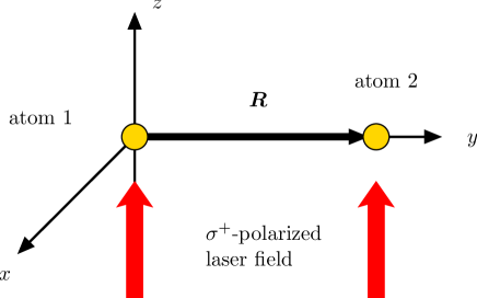
Figure 2: (Color online) Setup considered in Section III, which provides an illustration of the physical mechanisms responsible for the breakdown of the few-level approximation. In this example, an external laser field is used for the sake of illustration. Our main results starting from Section IV do not rely on external driving fields.

III Physical motivation

In the following Section IV, we will provide a rigorous treatment of the behavior of our model system under rotations of the atomic separation vector in order to study the geometrical properties of the different coupling terms in the master equation (7). In order to motivate this analysis, in this Section III, we will discuss a simple example for our results. This example employs an external laser field driving the atoms, which is used, however, only for the sake of illustration. Our main results starting from Section IV will not rely on external driving fields.

To this end, we consider the geometrical setup shown in Fig. 2. The atoms with internal structure as in Fig. 1 are aligned along the $y$ axis, and in addition to the model considered so far, a $\sigma^{+}$ polarized laser beam with Rabi frequency $\Omega_{L}$ and frequency $\omega_{L}$ propagates in $z$-direction. In rotating-wave approximation, the atom-laser interaction Hamiltonian reads

$$H_{L}=\hbar\sum\limits_{\mu=1}^{2}\left\{\Omega_{L}\,S_{3\,+}^{(\mu)}\,e^{-i\omega_{L}t}\,+\,\text{H.c.}\right\}\,.$$

The transition operators $S_{i\,+}^{(\mu)}$ are defined in Eq. (1). Since the laser polarization is $\sigma^{+}$, it couples only to the transition $|3\rangle\leftrightarrow|4\rangle$ in each atom. To describe this setup, one might be tempted to employ the usual few-level approximation, and thus neglect the excited states $|1\rangle$ and $|2\rangle$ in each atom, since they are not populated by the laser field. If this were correct, the seemingly relevant subsystem would be

$$S=\text{Span}(|4,4\rangle,\,|3,3\rangle,\,|3,4\rangle,\,|4,3\rangle)\,.$$

However, it is easy to prove that the state space of the two atoms can not be reduced to the subspace $S$, i.e., that the few-level approximation cannot be applied in its usual form. In order to show this, we include the atom-laser interaction into the master equation (7) and transform the resulting master equation in a frame rotating with the laser frequency. This equation is solved numerically with the initial condition $\varrho(t=0)=|4,4\rangle\langle 4,4|$, i.e. it is assumed that both atoms are initially in their ground states.

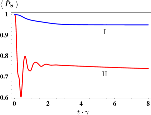
Figure 3: (Color online) Population in the subspace $S$ obtained by applying the few-level approximation to the setup in Fig. 2. The common parameters are $\theta=\pi/2$, $\phi=\pi/2$, $\delta=0$. Further, in (I), $\Omega_{L}=2\gamma$, $R=0.3\,\lambda_{0}$, and $\Delta=0.58\,\gamma$, where $\Delta=\omega_{L}-\omega_{0}$. Curve (II) shows the case $\Omega_{L}=5.4\,\gamma$, $R=0.1\,\lambda_{0}$, and $\Delta=5.2\,\gamma$.

Figure 3 shows the total population confined to the subspace $S$,

$$\big{\langle}\,\hat{P}_{S}\,\big{\rangle}=\text{Tr}\left[\varrho(t)\,\hat{P}_{S}\right]\,,$$ (16)

where ${P}_{S}$ is the projector onto the subspace $S$. It can easily be seen that for both sets of parameters, population is lost from the subspace $S$. Since all states but the excited states $|1\rangle$ and $|2\rangle$ are contained in $S$, it is clear that it is not sufficient to take only the excited state $|3\rangle$ into account in the usual few-level approximation.

The explanation of this outcome is straightforward. According to Eq. (8), the dipole transition $|3\rangle$ $\leftrightarrow|4\rangle$ of one atom is coupled by the cross-coupling term $\Omega_{31}$ to the $|1\rangle\leftrightarrow|4\rangle$ transition of the other atom. This coupling results in a population of state $|1\rangle$, even though the transition dipoles of the two considered transitions are orthogonal. Consequently, the dipole-dipole interaction between transitions with orthogonal dipole moments will result in the (partial) population of the states $|1,1\rangle$, $|1,3\rangle$, $|3,1\rangle$, $|1,4\rangle$, $|4,1\rangle$, although none of these states is directly coupled to the laser field.

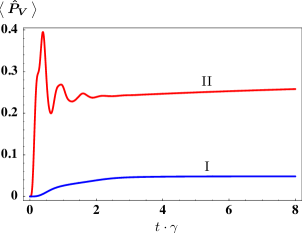
Figure 4: (Color online) Population of the subspace $V$, which contains all population which was lost from subspace $S$ in Fig. 3, such that the population in $S+V$ remains unity for all times. The parameters are as in Fig. 3.

The numerical verification of these statements is shown in Figure 4, which depicts the population of the subspace

$$V=\text{Span}(|1,1\rangle,\,|1,3\rangle,\,|3,1\rangle,\,|1,4\rangle,\,|4,1\rangle)\,.$$

$\hat{P}_{V}$ is the projector onto the subspace $V$, and the parameters are the same as above. Note that we have verified that all population is contained in the subspace $S+V$, i.e. $\big{\langle}\,\hat{P}_{S}\,\big{\rangle}+\big{\langle}\,\hat{P}_{V}\,\big{\rangle}=1$ at all times.

It is important to note that the sufficient subspace $S+V$ still does not contain all possible states of the two atoms, because the excited state $|2\rangle$ of each atom is neglected. The justification for this is that in the chosen geometry, the cross-coupling terms $\Omega_{21}$, $\Gamma_{21}$ and $\Omega_{32}$, $\Gamma_{32}$ vanish such that the transition $|2\rangle\leftrightarrow|4\rangle$ of one atom is not coupled to the transitions $|1\rangle\leftrightarrow|4\rangle$ and $|3\rangle\leftrightarrow|4\rangle$ of the other atom, see Eqs. (14) and (15). This is important since it demonstrates that it is also not correct to simply state that all atomic states have to be taken into account for all parameter configurations.

The above example clearly demonstrates that the few-level approximation is rendered impossible by the coupling terms between transitions with orthogonal dipole moments. Therefore, it is the nature of the dipole-dipole coupling itself which enforces that generally all Zeeman sublevels have to be taken into account, and not the polarization of the external laser fields, as one may be tempted to assume in the usual few-level approximation.

A physical interpretation for the origin of the vacuum-induced coupling of transitions with orthogonal dipole moments has been given in Evers et al. (2006). In essence, these couplings occur if the polarization of a (virtual) photon emitted on one of the transitions in the first atom has non-zero projection on different dipole moments of the second atom. Pictorially, then the second atom cannot measure the polarization of the photon, and thus has finite probability to absorb it also on transitions with dipole moments orthogonal to the dipole of the emitting transition.

IV Breakdown of the Few-Level Approximation

In this section, we return to our original setup in Fig. 1, and thus drop the external driving fields employed in Sec. III. We first derive a general statement about the behavior of the master equation (7) under rotations of the separation vector $\boldsymbol{R}$. On first sight, we will prove an obvious result: In the absence of external fields but the isotropic vacuum, there is no distinguished direction in space. Thus one expects the eigenenergies of the system to be invariant under rotations of $\boldsymbol{R}$, and this is indeed what we find. But despite its intuitiveness, this statement needs proof, and the discussion of the proof and its assumptions will provide the theoretical foundation for our central results and physical interpretations in the following sections.

IV.1 Central theorem

In addition to a given relative position $\boldsymbol{R}$ of the two atoms, we consider a different geometrical setup where the separation vector $\boldsymbol{P}$ is obtained from $\boldsymbol{R}$ by a rotation, $\boldsymbol{P}=\mathcal{R}_{\boldsymbol{u}}(\alpha)\boldsymbol{R}$. Here, $\mathcal{R}_{u}(\alpha)$ is an orthogonal $3\times 3$ matrix that describes a rotation in the three-dimensional real vector space $\mathbb{R}^{3}$ around the axis $\boldsymbol{u}$ by an angle $\alpha$. Our aim is to show that there exists a unitary operator $W$ such that

$$H_{\Omega}(\boldsymbol{P})=WH_{\Omega}(\boldsymbol{R})W^{\dagger}\,,$$ (17a)

$$\mathcal{L}_{\gamma}(\boldsymbol{P})\varrho=W\left[\mathcal{L}_{\gamma}(\boldsymbol{R})W^{\dagger}\varrho W\right]W^{\dagger}\,,$$ (17b)

where $W=W_{\boldsymbol{u}}(\alpha)$ is given by

$$W_{\boldsymbol{u}}(\alpha)=\exp[-i\alpha\;\boldsymbol{J}^{(1)}\cdot\boldsymbol{u}/\hbar]\exp[-i\alpha\;\boldsymbol{J}^{(2)}\cdot\boldsymbol{u}/\hbar]\,.$$ (18)

Here the operator $\exp[-i\alpha\;\boldsymbol{J}^{(\mu)}\cdot\boldsymbol{u}/\hbar]$ describes a rotation around the axis $\boldsymbol{u}$ by an angle $\alpha$ in the state space of atom $\mu$. The notation $H_{\Omega}(\boldsymbol{R})$ and $\mathcal{L}_{\gamma}(\boldsymbol{R})$ means that the coupling constants and collective decay rates in Eqs. (8) and (11) have to be evaluated at $\boldsymbol{R}$.

We proceed with the proof of Eq. (17). In a first step, we introduce the auxiliary operator $A_{\boldsymbol{R}}=WV_{\boldsymbol{R}}W^{\dagger}$, where $V_{\boldsymbol{R}}$ is the interaction Hamiltonian for a relative position of the atoms given by $\boldsymbol{R}$, and $W=W_{\boldsymbol{u}}(\alpha)$ is defined in Eq. (18). The evaluation of $A_{\boldsymbol{R}}$ involves only the transformation of the dipole operator of each atom. Since the matrix elements of vector operators transform like classical vectors under rotations (see, e.g., Sec. 3.10. in Sakurai (1994)), we find

$$W\;\boldsymbol{\hat{d}}^{(\mu)}\;W^{\dagger}=\sum\limits_{i=1}^{3}\big{[}\boldsymbol{\tilde{d}}_{i}\;S_{i\,+}^{(\mu)}+\text{H.c.}\big{]}\,,$$ (19)

where $\boldsymbol{\tilde{d}}_{i}=\mathcal{R}_{\boldsymbol{u}}^{-1}(\alpha)\boldsymbol{d}_{i}$. This shows that the only difference between the auxiliary operator $A_{\boldsymbol{R}}$ and $V_{\boldsymbol{R}}$ is that the dipole moments of the former are determined by $\boldsymbol{\tilde{d}}_{i}$ instead of $\boldsymbol{d}_{i}$.

In a second step, we employ the tensor properties of $\overset{\leftrightarrow}{\chi}$ to find the following expression for the parameters $\Omega_{ij}(\boldsymbol{P})$ and $\Gamma_{ij}(\boldsymbol{P})$ [see Eqs. (9) and (12)],

$$\hbar\Omega_{ij}(\boldsymbol{P})= \left[\mathcal{R}_{\boldsymbol{u}}^{-1}(\alpha)\boldsymbol{d}_{i}\right]^{\text{T}}\overset{\leftrightarrow}{\chi}_{\text{re}}(\boldsymbol{R})\left[\mathcal{R}_{\boldsymbol{u}}^{-1}(\alpha)\boldsymbol{d}_{j}^{*}\right],$$ (20)

$$\hbar\Gamma_{ij}(\boldsymbol{P})= \left[\mathcal{R}_{\boldsymbol{u}}^{-1}(\alpha)\boldsymbol{d}_{i}\right]^{\text{T}}\overset{\leftrightarrow}{\chi}_{\text{im}}(\boldsymbol{R})\left[\mathcal{R}_{\boldsymbol{u}}^{-1}(\alpha)\boldsymbol{d}_{j}^{*}\right].$$ (21)

This important result shows that a rotation of the dipole moments $\boldsymbol{d}_{i}$ by $\mathcal{R}_{\boldsymbol{u}}^{-1}(\alpha)$ is formally equivalent to a rotation of $\boldsymbol{R}$ by $\mathcal{R}_{\boldsymbol{u}}(\alpha)$ in the master equation (7).

From the combination of the results obtained in step one and two, we conclude that the exchange of $V_{\boldsymbol{R}}$ by $A_{\boldsymbol{R}}$ in the integral of Eq. (6) is equivalent to a rotation of the separation vector from $\boldsymbol{R}$ to $\boldsymbol{P}=\mathcal{R}_{\boldsymbol{u}}(\alpha)\boldsymbol{R}$,

$$I =\frac{-1}{\hbar^{2}}\int\limits_{0}^{t}d\tau\text{Tr}_{\text{F}}\Big{(}\big{[}A_{\boldsymbol{R}},\big{[}U(\tau)A_{\boldsymbol{R}}U^{\dagger}(\tau),\tilde{\varrho}(\hat{\tau})\big{]}\big{]}\Big{)}$$ (22)

$$=-\frac{i}{\hbar}[H_{\Omega}(\boldsymbol{P}),\varrho]+\mathcal{L}_{\gamma}(\boldsymbol{P})\varrho\,,$$ (23)

where $\hat{\tau}=t-\tau$ and

$$\tilde{\varrho}(\hat{\tau})=U(\tau)\left[\varrho_{\text{F}}\otimes\varrho(\hat{\tau})\right]U^{\dagger}(\tau)\,.$$ (24)

Note that the equality of Eqs. (22) and (23) holds under the same assumptions that led from Eqs. (6) to (7).

In the second part of the proof we evaluate the integral in Eq. (22) in a different way. In the discussion following Eq. (10), we justified that $\mathcal{L}_{\gamma}$ and $H_{\Omega}$ depend only on the mean transition frequency $\omega_{0}$. Here we employ exactly the same approximation rem and replace the frequencies $\omega_{i}$ appearing in $U(\tau)A_{\boldsymbol{R}}U^{\dagger}(\tau)$ by $\omega_{0}$. Since $H_{\text{A}}$ commutes with $\boldsymbol{J}^{(\mu)}$ if all frequencies $\omega_{i}$ are replaced by the mean transition frequency $\omega_{0}$, we have $[W,U]=0$ and hence

$$U(\tau)A_{\boldsymbol{R}}U^{\dagger}(\tau)=WU(\tau)V_{\boldsymbol{R}}U^{\dagger}(\tau)W^{\dagger}\,.$$ (25)

It follows that the argument of the trace in Eq. (22) can be written as

$$W\big{[}V_{\boldsymbol{R}},\,\big{[}U(\tau)V_{\boldsymbol{R}}U^{\dagger}(\tau),W^{\dagger}\tilde{\varrho}(\hat{\tau})W\big{]}\big{]}W^{\dagger}\,.$$ (26)

In contrast to Eq. (22), the double commutator contains now the original interaction Hamiltonian $V_{\boldsymbol{R}}$ that corresponds to a setting with separation vector $\boldsymbol{R}$. We thus obtain

$$I=-\frac{i}{\hbar}[WH_{\Omega}(\boldsymbol{R})W^{\dagger},\varrho]+W\left[\mathcal{L}_{\gamma}(\boldsymbol{R})W^{\dagger}\varrho W\right]W^{\dagger}\,.$$ (27)

Finally, the comparison of Eqs. (27) and (23) establishes Eq. (17) which concludes the proof.

Note that throughout this proof, we have not made reference to the specific type of the Zeeman sublevels employed in our example shown in Fig. 1. Therefore, the central theorem holds for transitions between states with arbitrary angular momentum structure, as long as complete multiplets are considered.

IV.2 Diagonalization of $H_{\Omega}$

We now turn to the discussion of Eq. (17), which will lead to our central results. The Hamiltonian $H_{\Omega}$ describes the coherent part of the dipole-dipole interaction between the atoms. From Eq. (17a), it is immediately clear that the eigenvalues of $H_{\Omega}$ depend only on the interatomic distance, but not on the orientation of the separation vector $\boldsymbol{R}$. The reason is that the spectrum of two operators, which are related by a unitary transformation, is identical. In our case, the Hamiltonian $H_{\Omega}(\boldsymbol{R})$ and $H_{\Omega}(\boldsymbol{P})$ for different orientations $\boldsymbol{R}$ and $\boldsymbol{P}$ are related by the unitary transformation $W$, and since $\boldsymbol{P}$ is obtained from $\boldsymbol{R}$ by an arbitrary rotation, the eigenvalues of $H_{\Omega}$ are identical for any orientation.

Next we re-obtain this result in a more explicit way and derive symbolic expressions for the eigenvalues and eigenstates of $H_{\Omega}$. This Hamiltonian can be written as

$$H_{\Omega}=\sum\limits_{i,j=1}^{3}\big{(}\;[H_{\Omega}]^{\mathcal{S}}_{ij}\;|s_{i}\rangle\langle s_{j}|+[H_{\Omega}]^{\mathcal{A}}_{ij}\;|a_{i}\rangle\langle a_{j}|\;\big{)}\,,$$ (28)

where the symmetric and antisymmetric states are defined as

$$|s_{i}\rangle =(\,|i,4\rangle+|4,i\rangle\,)/\sqrt{2}\,,$$ (29a)

$$|a_{i}\rangle =(\,|i,4\rangle-|4,i\rangle\,)/\sqrt{2}\,,$$ (29b)

and $|i,j\rangle=|i_{1}\rangle\otimes|j_{2}\rangle$. Since all matrix elements $\langle s_{i}|H_{\Omega}|a_{j}\rangle$ of $H_{\Omega}$ between a symmetric and an antisymmetric state vanish, the set of eigenstates decomposes into a symmetric subspace $\mathcal{S}$ and an antisymmetric subspace $\mathcal{A}$. The matrix elements of $H_{\Omega}$ in the subspace $\mathcal{S}$ spanned by the symmetric states $\{|s_{1}\rangle,\,|s_{2}\rangle,\,|s_{3}\rangle\}$ are

$$[H_{\Omega}]^{\mathcal{S}} =-\hbar\left(\begin{array}[]{r@{\hspace{0.5cm}}r@{\hspace{0.5cm}}r }\Omega_{11}\hskip 14.22636pt&\Omega_{21}^{*}\hskip 14.22636pt&\Omega_{31}^{*}\\ \Omega_{21}\hskip 14.22636pt&\Omega_{22}\hskip 14.22636pt&\Omega_{32}^{*}\\ \Omega_{31}\hskip 14.22636pt&\Omega_{32}\hskip 14.22636pt&\Omega_{33}\end{array}\right)\,,$$ (33)

and the representation of $H_{\Omega}$ in the subspace $\mathcal{A}$ spanned by the antisymmetric states $\{|a_{1}\rangle,\,|a_{2}\rangle,\,|a_{3}\rangle\}$ is given by $[H_{\Omega}]^{\mathcal{A}}=-[H_{\Omega}]^{\mathcal{S}}$. Note that the collective ground state $|4,4\rangle$ and the states $|i,j\rangle$ ($i,j\in\{1,2,3\}$) where each atom is in an excited state are not influenced by the dipole-dipole interaction and thus not part of the expansion (28).

In Section IV.1, we have derived a general relation between any two orientations of the interatomic distance vector. In order to apply this result, we define the vector $\boldsymbol{R}_{z}$ to be parallel to the $z$ axis, i.e. $\boldsymbol{R}_{z}=R\,\boldsymbol{e}_{z}$. This corresponds to the choice $\theta=0$ in Eq. (13). Any separation vector $\boldsymbol{P}$ can then be obtained from $\boldsymbol{R}_{z}$ as $\boldsymbol{P}=\mathcal{R}_{\boldsymbol{u}}(\alpha)\boldsymbol{R}_{z}$ by a suitable choice of the rotation axis $\boldsymbol{u}$ and the angle $\alpha$.

We then proceed with the diagonalization of the Hamiltonian $H_{\Omega}(\boldsymbol{R}_{z})$ with atomic separation vector $\boldsymbol{R}_{z}$. The explicit calculation of the coupling constants $\Omega_{ij}$ shows that the off-diagonal elements in Eq. (33) vanish if the atoms are aligned along the $z$ axis, see Eqs. (14) and (15) with $\theta=0$. It follows that the Hamiltonian $H_{\Omega}(\boldsymbol{R}_{z})$ is already diagonalized by the symmetric and antisymmetric states Eq. (29), and the eigenvalues of $[H_{\Omega}]^{\mathcal{S}}$ and $[H_{\Omega}]^{\mathcal{A}}$ are given by $\lambda^{\mathcal{S}}_{i}=-\hbar\Omega_{ii}(\boldsymbol{R}_{z})$ and $\lambda^{\mathcal{A}}_{i}=\hbar\Omega_{ii}(\boldsymbol{R}_{z})$, respectively.

According to Eq. (17a), the Hamiltonian $H_{\Omega}(\boldsymbol{P})$ is the unitary transform of $H_{\Omega}(\boldsymbol{R}_{z})$ by $W$. The normalized eigenstates of $H_{\Omega}(\boldsymbol{P})$ are thus determined by $W|s_{i}\rangle$ and $W|a_{i}\rangle$, and their eigenvalues are again $\lambda^{\mathcal{S}}_{i}$ and $\lambda^{\mathcal{A}}_{i}$ , respectively. Since the orientation of $\boldsymbol{P}$ is arbitrary, the eigenvalues of $H_{\Omega}(\boldsymbol{P})$ depend only on the interatomic distance $|\boldsymbol{P}|=|\boldsymbol{R}_{z}|=R$, but not on the orientation of the separation vector.

Thus, it follows from our theorem in Sec. IV.1 that the eigenvalues of $H_{\Omega}(\boldsymbol{P})$ are invariant under rotation of the interatomic distance vector.

IV.3 Diagonalization of $H_{\text{A}}+H_{\Omega}$

An additional conclusion can be drawn from Eq. (17) if the operator $H_{\text{A}}$ commutes with the transformation $W=W_{\boldsymbol{u}}(\alpha)$, i.e.,

$$[H_{\text{A}},W]=0\,.$$ (34)

Then, Eq. (17a) implies that $H_{\text{A}}+H_{\Omega}(\boldsymbol{P})$ is the unitary transform of $H_{\text{A}}+H_{\Omega}(\boldsymbol{R})$ by $W$. A straightforward realization of this is the case of vanishing Zeeman splitting $\delta$, in which the relation holds for an arbitrary orientation of $\boldsymbol{P}$. Then, the energy levels of the full system Hamiltonian $H_{\text{A}}+H_{\Omega}$ do not depend on the orientation of the separation vector.

This result can be understood as follows. In the absence of a magnetic field ($\delta=0$), there is no distinguished direction in space. Since the vacuum is isotropic in free space, one expects that the energy levels of the system are invariant under rotations of the separation vector $\boldsymbol{R}$.

By contrast, the application of a magnetic field in $z$ direction breaks the full rotational symmetry. For $\delta\not=0$, the atomic Hamiltonian $H_{\text{A}}$ only commutes with transformations $W_{\boldsymbol{u}}(\alpha)$ that correspond to a rotation of the separation vector around the $z$ axis, $\boldsymbol{u}=\boldsymbol{e}_{z}$. If we express the atomic separation vector in terms of spherical coordinates as in Eq. (13), this means that the eigenvalues of the full system Hamiltonian $H_{\text{A}}+H_{\Omega}$ do only depend on the interatomic distance $R$ and the angle $\theta$, but not on the angle $\phi$. This result reflects the symmetry of our system with respect to rotations around the $z$ axis.

IV.4 Unitary equivalence of time evolution in different orientations

If the operator $H_{\text{A}}$ commutes with the transformation $W=W_{\boldsymbol{u}}(\alpha)$, another conclusion can be drawn. Then, the result in Eq. (17) implies that the density operator $W\varrho(\boldsymbol{R})W^{\dagger}$ obeys the same master equation than $\varrho(\boldsymbol{P})$ for $\boldsymbol{P}=\mathcal{R}_{\boldsymbol{u}}(\alpha)\boldsymbol{R}$. It follows that $\boldsymbol{P}$ is the unitary transform of $\varrho(\boldsymbol{R})$ by $W$, i.e.

$$\varrho(\boldsymbol{P})=W\varrho(\boldsymbol{R})W^{\dagger}\,.$$ (35)

As discussed in Sec. IV.3, the free atomic Hamiltonian $H_{\text{A}}$ commutes with $W_{\boldsymbol{u}}(\alpha)$ for an arbitrary choice of the rotation axis $\boldsymbol{u}$ and angle $\alpha$ if the Zeeman splitting $\delta$ vanishes.

We thus conclude that it suffices to determine the solution of the master equation (7) for only one particular geometry if $\delta=0$. Any other solution can then be generated simply by applying the transformation $W=W_{\boldsymbol{u}}(\alpha)$ with suitable values of $\boldsymbol{u}$ and $\alpha$ to the solution for the particular geometry.

IV.5 Establishment of the breakdown

In Secs. IV.2-IV.4, we presented several results concerning the energy levels and the time evolution of the two dipole-dipole interacting atoms that are based on the central theorem in Eq. (17). However, this theorem can only be established if each atom is modelled by complete sets of angular momentum multiplets, and represents the reference case that corresponds to results which can be expected in an experiment. If any of the Zeeman sublevels of the $P_{1}$ triplet are neglected, the unitary operator $W$ does not exist since it is impossible to define an angular momentum or vector operator in a state space where magnetic sublevels have been removed artificially. In this case, the central statement cannot be applied. Still, the system can be solved without the help of the theorem. The breakdown of the few-level approximation for collective systems is then established by noting that the results for systems with artificially reduced state space fail to recover the results derived in Secs. IV.2-IV.4 for the full system.

In order to illustrate this point in more detail, we consider the system in Fig. 1 and assume that the excited states of each atom are degenerate ($\delta=0$). According to our findings in Secs. IV.2 and IV.3, the energy levels of the complete system depend on the length of the separation vector $\boldsymbol{R}$, but not on its orientation. In contrast, the omission of any of the Zeeman sublevels leads to a spurious dependence of the energy levels on the orientation, and thus to incorrect predictions.

For example, if the excited states $|1\rangle$ and $|3\rangle$ in each atom are omitted, the level scheme in Fig. 1(b) reduces to an effective two-level system comprised of the states $|2\rangle$ and $|4\rangle$. The collective two-atom system is then described by the ground state $|4,4\rangle$, the excited state $|2,2\rangle$ and the symmetric and antisymmetric states $|s_{2}\rangle$ and $|a_{2}\rangle$. The frequency splitting between the states $|s_{2}\rangle$ and $|a_{2}\rangle$ is given by $2|\Omega_{22}|$, where

$$\Omega_{22}=\frac{3}{2}\gamma_{2}\left[f_{1}(\eta)-\cos^{2}(\theta)f_{2}(\eta)\right]\,,$$ (36)

and

$$f_{1}(\eta) =\left(\frac{1}{\eta}-\frac{1}{\eta^{3}}\right)\cos\eta-\frac{1}{\eta^{2}}\sin\eta\,,$$ (37)

$$f_{2}(\eta) =\left(\frac{1}{\eta}-\frac{3}{\eta^{3}}\right)\cos\eta-\frac{3}{\eta^{2}}\sin\eta\,.$$ (38)

Since the second term in Eq. (36) is proportional to $\cos^{2}\theta$, the energy levels of the artificially created two-level system strongly depend on the orientation of the separation vector $\boldsymbol{R}$. This is at variance with our finding in Sec. IV.3, where we have shown that the energy levels do not depend on the orientation of the vector $\boldsymbol{R}$ if each atom consists of complete and degenerate Zeeman multiplets. We thus conclude that all Zeeman sublevels generally have to be taken into account.

Since the validity of the central theorem Eq. (17) is not restricted to the $S_{0}\leftrightarrow P_{1}$ transition discussed so far, it follows that the breakdown of the few-level approximation can be established for transitions between arbitrary angular momentum multiplets.

The intuitive explanation of the breakdown has already been hinted at in Sec. III. For a more formal discussion, we return to the matrix representation of $[H_{\Omega}]^{\mathcal{S}}$ in Eq. (33). The diagonal elements proportional to $\Omega_{ii}$ account for the coherent interaction between a dipole of one of the atoms and the corresponding dipole of the other atom. By contrast, the off-diagonal terms proportional to $\Omega_{ij}$ with $i\not=j$ arise from the vacuum-mediated interaction between orthogonal dipoles of different atoms Agarwal and Patnaik (2001); Evers et al. (2006). It is the presence of these terms that renders the simplification of the atomic level scheme impossible since they couple an excited state $|i\rangle$ of one atom to a different excited state $|j\rangle$ ($i\not=j$) of the other atom. A similar argument applies to the collective decay rates $\Gamma_{ij}$ appearing in $\mathcal{L}_{\gamma}\varrho$. Thus, if any Zeeman sublevel of the excited state multiplet is artificially removed, then some of these vacuum-induced couplings $\Omega_{ij}$ with $i\not=j$ are neglected, which leads to incorrect results. Now, it is also apparent why the breakdown of the few-level approximation appears exclusively in collective systems. For single atoms in free space, a coupling of orthogonal transition dipole moments via the vacuum is impossible.

IV.6 Recovery of the few-level approximation in special geometries

The identification of the vacuum-induced couplings $\Omega_{ij}$ and $\Gamma_{ij}$ between orthogonal transition dipole moments as the cause of the breakdown enables one to conjecture that few-level approximations are justified for particular geometrical setups, where some or all of the cross-coupling terms vanish.

For example, we mentioned earlier that all cross-coupling terms vanish if the atoms are aligned along the $z$ axis. This corresponds to the case $\theta=0$ in Eqs. (13)-(15). Then, the $S_{0}\leftrightarrow P_{1}$ transition may be reduced to a two-level system, formed by an arbitrary sublevel of the $P_{1}$ triplet and the ground state $S_{0}$.

As a second example, we assume the atoms to be aligned in the $x$-$y$-plane, i.e., $\theta=\pi/2$ in Eq. (13). Then the terms $\Omega_{21}$, $\Gamma_{21}$ and $\Omega_{32}$, $\Gamma_{32}$ vanish, see Eqs. (14)-(15). In effect, the excited state $|2\rangle$ may be disregarded such that the atomic level scheme simplifies to a V-system formed by the states $|1\rangle$ and $|3\rangle$ of the $P_{1}$ multiplet and the ground state $S_{0}$.

Note that the cross-coupling terms also become irrelevant in the special case $|\delta|\gg|\Omega_{ij}|,|\Gamma_{ij}|$ ($i\neq j$), see our discussion below Eq. (12).

V Discussion and summary

Throughout this article, we have studied the properties of various parts of the system Hamiltonian as well as the full density operator under rotations of the interatomic distance vector. This discussion was based on a general theorem in Sec. IV.1 which relates the system properties for different orientations of the interatomic distance vector.

First, we have discussed the Hamiltonian $H_{\Omega}$, which describes the coherent coupling between different transitions in the two atoms induced by the vacuum field. Armed with our main theorem, it is possible to first diagonalize $H_{\Omega}$ in a special geometry, where the eigenvectors and eigenenergies assume a particularly simple form. The eigenvectors and eigenenergies for an arbitrary system geometry are then derived via the theorem. Our main result of Sec. IV.2 is that the eigenvalues of $H_{\Omega}$ are invariant under rotation of the interatomic distance vector.

In a second step, we have studied the eigenenergies of the full system Hamiltonian $H_{A}+H_{\Omega}$, which in general are not invariant under rotation of the interatomic distance vector. The invariance, however, is recovered if $H_{\text{A}}$ commutes with the transformation $W=W_{\boldsymbol{u}}(\alpha)$, which is given in explicit form as a result of our theorem. Most importantly, this additional condition is fulfilled for a degenerate excited state multiplet, i.e., if the Zeeman splitting $\delta$ vanishes. Then, there is no preferred direction in space, such that the invariance of the eigenenergies, which are observables, can be expected.

We then conclude the breakdown of the few-level approximation in Sec. IV.5, since our results of the previous sections are violated if any of the excited state multiplet sublevels are artificially removed. Possible consequences are, for example, a spurious dependence of the eigenenergies on the orientation of the interatomic distance vector, and thus of all observables that depend on the transition frequencies among the various eigenstates of the system. In experiments, in addition, a loss of population from the subspace considered in the few-level approximation would be observed. Our proof can be generalized to transitions between arbitrary angular momentum multiplets.

We have identified the vacuum-induced dipole-dipole coupling between transitions with orthogonal dipole moments as the origin of the breakdown. On the one hand, this explains why the breakdown exclusively occurs in collective systems, since such orthogonal couplings are impossible in single atoms in free space. On the other hand, the interpretation enables one to identify special geometries where some of the Zeeman sublevels can be omitted. This also allows to connect our results to previous studies involving dipole-dipole interacting few-level systems. In these studies involving the few-level approximation, typically a very special geometry was chosen, e.g., with atomic separation vector and transition dipole moments orthogonal or parallel to each other. These results remain valid if a geometry can be found such that the full Zeeman sublevel scheme reduces to the chosen level scheme as discussed in Sec. IV.6. It should be noted, however, that there are physical realizations of interest which in general do not allow for a particular system geometry that leads to the validity of a few-level approximation, such as quantum gases.

Finally, on a more technical side, our results can also be applied to considerably simplify the computational effort required for the treatment of such dipole-dipole interacting multilevel systems with arbitrary alignment of the two atoms. First, our theorem both allows for a convenient evaluation of eigenvalues and eigenenergies for arbitrary orientations of the interatomic distance vector based on the results found in a single, special alignment. Second, we have found in Sec. IV.4 that for the degenerate system, the density matrices for different orientations are related to each other by the unitary transformation $W$ defined in our theorem. Thus the solution for any orientation can be obtained from a single time integration simply by applying this transformation.

References

- Scully and Zubairy (1997) M. O. Scully and M. S. Zubairy, Quantum Optics (Cambridge University Press, Cambridge, 1997).
- Ficek and Swain (2005) Z. Ficek and S. Swain, Quantum Interference and Coherence (Springer, New York, 2005).
- (3) G. S. Agarwal, in Quantum Statistical Theories of Spontaneous Emission and Their Relation to Other Approaches, edited by G. Höhler (Springer, Berlin, 1974).
- Jaynes and Cummings (1963) E. T. Jaynes and F. W. Cummings, Proc. IEEE 51, 89 (1963).
- Lamb et al. (1987) W. E. Lamb, R. R. Schlicher, and M. O. Scully, Phys. Rev. A 36, 2763 (1987).
- Thirunamachandran (1980) T. Thirunamachandran, Mol. Phys. 40, 393 (1980); D. O’Dell, S. Giovanazzi, G. Kurizki, and V. M. Akulin, Phys. Rev. Lett. 84, 5687 (2000); A. Gero and E. Akkermans, ibid. 96, 093601 (2006).
- DeVoe and Brewer (1996) R. G. DeVoe and R. G. Brewer, Phys. Rev. Lett. 76, 2049 (1996); J. Eschner, C. Raab, F. Schmidt-Kaler, and R. Blatt, Nature 413, 495 (2001).
- Kästel and Fleischhauer (2005) J. Kästel and M. Fleischhauer, Phys. Rev. A 71, 011804(R) (2005).
- Hettich et al. (2002) C. Hettich, C. Schmitt, J. Zitzmann, S. Kühn, I. Gerhardt, and V. Sandoghdar, Nature 298, 385 (2002).
- Barnes et al. (2005) M. D. Barnes, P. S. Krstic, P. Kumar, A. Mehta, and J. C. Wells, Phys. Rev. B 71, 241303(R) (2005).
- Lukin and Hemmer (2000) M. D. Lukin and P. R. Hemmer, Phys. Rev. Lett. 84, 2818 (2000); A. Beige, S. F. Huelga, P. L. Knight, M. B. Plenio, and R. C. Thompson, J. Mod. Opt. 47, 401 (2000); G. K. Brennen, C. M. Caves, P. S. Jessen, and I. H. Deutsch, Phys. Rev. Lett. 82, 1060 (1999); A. Barenco, D. Deutsch, A. Ekert, and R. Jozsa, ibid. 74, 4083 (1995).
- Sakurai (1994) J. J. Sakurai, Modern Quantum Mechanics (Addison-Wesley, Reading, MA, 1994).
- Agarwal and Patnaik (2001) G. S. Agarwal and A. K. Patnaik, Phys. Rev. A 63, 043805 (2001).
- Evers et al. (2006) J. Evers, M. Kiffner, M. Macovei, and C. H. Keitel, Phys. Rev. A 73, 023804 (2006).
- (15) Note that appearing in the free evolution term of the master equation is not approximated.
- (16) M. Kiffner, J. Evers and C. H. Keitel, Phys. Rev. A 75, 032313 (2007).