Simulating a single qubit channel using a mixed state environment

Abstract

We analyze the class of single qubit channels with the environment modeled by a one-qubit mixed state. The set of affine transformations for this class of channels is computed analytically, employing the canonical form for the two-qubit unitary operator. We demonstrate that, $\frac{3}{8}$ of the generalized depolarizing channels can be simulated by the one-qubit mixed state environment by explicitly obtaining the shape of the volume occupied by this class of channels within the tetrahedron representing the generalized depolarizing channels. Further, as a special case, we show that the two-Pauli Channel cannot be simulated by a one-qubit mixed state environment.

I Introduction

The storage and transmission of quantum states in a decohering environment is unavoidable in quantum computation and quantum communication  G.M.Palma (1996); Zurek (2003); Nielsen and Chuang (2000). The conceptual device of a quantum channel is very useful in addressing the issues of such a transmission Schumacher (1996) and to analyze decoherence related questions in quantum cryptography Gisin et al. (2002) and quantum teleportation Bowen and Bose (2001); Yeo (2003).

A general quantum operation on an $n$-dimensional quantum system is a completely positive map. Such a map defines a quantum channel for the given system and can be formally represented by its operator sum representation Sudarshan et al. (1961); Choi (1975); Karus (1983). One can also look at this general quantum evolution using affine transformations for the channel Jordan (2005). In an explicit model for this evolution, the system is considered as a part of a larger closed system undergoing unitary evolution. The part of this larger system that we are not interested in can be thought of as the environment, which when traced over, gives us the dynamics of the effective sub-system. The environment can in general be very large. However, it turns out that in order to achieve the most general evolution for a system with an $n$-dimensional Hilbert space, we need an environment which is of dimensions $n^{2}$ (if we allow the most general unitary evolution of the total system and assume that the initial state of the environment is pure) Schumacher (1996). Therefore, to simulate the most general evolution of a single qubit, at least a four-dimensional (two-qubit) environment is required. However if we allow the initial state of the environment to be a mixed state, there is a possibility of achieving such a simulation by employing a smaller environment. This reduction in the dimension of the Hilbert space is desirable for performing actual simulations of open quantum systems Terhal et al. (1999). Along these lines, an argument based on counting the number of independent parameters suggests that a one-qubit mixed state environment might be sufficient to simulate the most general quantum evolution of a single qubit Lloyd (1996). Further investigations in this direction have revealed that there are counter-examples to the above conjecture, and there are single qubit channels which cannot be simulated by one qubit in the environment Terhal et al. (1999); Zalka and Rieffel (2002); Bacon et al. (2001).

We investigate this question in detail via a different route and compute the set of affine transformations for this class of channels analytically, employing the canonical form for two-qubit unitary operators Kraus and Cirac (2001). Restricting ourselves to generalized depolarizing channels, we show that a sizable volume (namely $\frac{5}{8}$) of these channels cannot be simulated by a one-qubit mixed state environment. Further, we show that the counter example of the two-Pauli channel found by Terhal et. al. is a special case of our results.

The material in this paper is arranged as follows: in Section II, we explain how a one-qubit mixed state environment can be considered for the simulation of a single qubit channel and the significance of modeling the channel using such an environment. We consider the two-qubit unitary required for the simulation of such a channel and discuss how this class of channels could be a candidate that could occupy a sizable volume in the space of single-qubit channels. At the end of this section, the expression for the affine transformation for a general single qubit channel modeled using a one-qubit mixed state environment is obtained. In section III we take up the special case of generalized depolarizing channels. The affine transformation for this case is obtained by setting the shift of the Bloch sphere origin to zero in the general expression for affine transformation developed in Section II. These channels are classified by computing their singular values. From the structure of these singular values and the analysis of all the possible cases the volume occupied by the generalized depolarizing channels simulated by a one-qubit mixed state environment is computed and compared to the total volume of generalized depolarizing channels. The section concludes with a discussion of the two-Pauli Channel considered as a special case of generalized depolarizing channels and it is shown that it cannot be simulated by a one-qubit mixed state environment. Section IV contains some concluding remarks.

II One-qubit channels with a one-qubit mixed state as the environment

In the model for the one-qubit channel that we consider, we allow the qubit of interest to interact with only one environment qubit. The interaction unitary is allowed to be the most general two-qubit unitary and the environment qubit is a general mixed state. This channel is schematically depicted in Figure (1).

For the purpose of characterizing the channel, we consider the system qubit to be in a general pure state (a point on the Bloch sphere) given by

$$|\psi\rangle=\cos{\frac{\theta}{2}}|0\rangle+e^{-i\phi}\sin{\frac{\theta}{2}}|1\rangle$$ (1)

where $\theta$ varies from 0 to $\pi$ and $\phi$ varies from 0 to 2$\pi$.

The environment qubit is assumed to be in a general mixed state for which we choose a particular parameterization as follows:

$$\rho_{e}=(1-\lambda)\,\frac{I}{2}+\lambda\,|\phi\rangle\langle\phi|$$ (2)

where $\frac{I}{2}$ corresponds to a maximally mixed state and $|\phi\rangle$ corresponds to a general pure state given by

$$|\phi\rangle=\cos{\frac{\xi}{2}}|0\rangle+e^{-i\eta}\sin{\frac{\xi}{2}}|1\rangle$$ (3)

where $\xi$ varies from $0$ to $\pi$ and $\eta$ varies from $0$ to $2\pi$. Therefore, the environment state can be thought of as a mixture of a completely mixed state and a pure state. The parameter $\lambda$ indicates the degree to which the state is mixed. By varying $\lambda$ from $1$ to $0$, we can go from a pure to a maximally mixed state of the environment.

Figure 1: Implementation of a one-qubit channel using a single qubit mixed state environment. The system is taken to be in a pure initial state $|\psi\rangle$ while the environment is in a mixed state $\rho_{e}$. The interaction takes place via the two-qubit unitary $U_{d}$ and the environment qubit is discarded after the interaction.

The interaction that takes place between the system qubit and the environment qubit corresponds to a general unitary operator in the four-dimensional (two-qubit) Hilbert space. This most general unitary which is an $SU(4)$ transformation has fifteen independent parameters. However, it has been shown that an arbitrary two-qubit unitary can be decomposed into local unitaries on each qubit sandwiching a non-trivial interaction unitary. This interaction unitary $U_{d}$ belongs to a three-parameter family of transformations Kraus and Cirac (2001).

$$U=(U_{1}\otimes V_{1})\,U_{d}\,(U_{2}\otimes V_{2})$$

$$U\in SU(4);\,{\rm and}\,U_{1},U_{2},V_{1},V_{2}\in SU(2)$$ (4)

This is pictorially shown in Figure 2.

This three-parameter family of interaction unitaries has the power to entangle or unentangle the qubits involved. This family finds a simple diagonal representation in the special Bell basis, namely

$$U^{\rm Bell}_{d}=\sum e^{-i\lambda_{i}}|\psi_{i}\rangle\langle\psi_{i}|.$$ (5)

where $|\psi_{j}$ for $j=1,2,3,4$ are the special Bell basis vectors Bennett et al. (1996). The number of independent parameters $\lambda_{j}$ can be reduced to three by a global phase change.

This transformation matrix can be readily transformed into the product basis $\{|00\rangle,|01\rangle,|10\rangle,|11\rangle\}$ to obtain

$$U_{d}^{\rm Prod}\!=\!\left(\!\begin{array}[]{cccc}\cos{\frac{\alpha+\gamma}{2}}&0&0&\!\!i\sin{\frac{\alpha+\gamma}{2}}\cr 0&\!\!\!\!\!\!\cos{\frac{\alpha-\gamma}{2}}e^{-i\beta}&i\sin{\frac{\alpha-\gamma}{2}}e^{-i\beta}&0\cr 0&\!\!\!\!\!\!i\sin{\frac{\alpha-\gamma}{2}}e^{-i\beta}&\cos{\frac{\alpha-\gamma}{2}}e^{-i\beta}&0\cr i\sin{\frac{\alpha+\gamma}{2}}&0&0&\!\!\cos{\frac{\alpha+\gamma}{2}}\end{array}\!\right)$$ (6)

where

$$\alpha = \phantom{-}(\lambda_{1}-\lambda_{2}-\lambda_{3}+\lambda_{4})/2,$$

$$\beta = -(\lambda_{1}+\lambda_{2}+\lambda_{3}+\lambda_{4})/2,$$

$$\gamma = \phantom{-}(\lambda_{1}-\lambda_{2}+\lambda_{3}-\lambda_{4})/2$$ (7)

We are considering a quantum channel for a single qubit with another qubit acting as the environment and a general unitary transformation (described above) providing the interaction between the two qubits. It is easy to see that the properties of the channel do not change with the local unitary transformations $U_{1},V_{1}$ and $U_{2},V_{2}$. Therefore, for the analysis of the family of such channels, the interaction unitary that needs to be considered is the three-parameter family given in (LABEL:ch9_t). The final output state of the system $\rho_{\rm out}$ emerging from the channel after the action of $U_{d}$ is obtained by tracing over the environment qubit.

Figure 2: Schematic Diagram for a two-qubit unitary. The local unitaries $U_{1},V_{1},U_{2},V_{2}$ together with $U_{d}$, which is diagonal in the special Bell basis, provide a decomposition of a general $SU(4)$ transformation.

Mathematically, a one-qubit channel can be described in a number of ways, and we find it useful to picture it in terms of an affine transformation of the Bloch sphere. The quantum states of a single qubit on the Bloch sphere can be represented as follows:

$$\rho=\frac{1}{2}(I+{\mathbf{n}.\sigma})$$ (8)

where the $\sigma$’s are Pauli matrices, and ${\mathbf{n}}$ is a 3-component real vector. For pure states $|{\mathbf{n}}|=1$, and for mixed states $|{\mathbf{n}}|<1$. Any arbitrary trace-preserving quantum operation on (8) is given by a map of the form $\rho\rightarrow\rho^{\prime}$, with the new vector determining $\rho^{\prime}$ given by

$$n_{i}^{\prime}=\sum^{3}_{j=1}M_{ij}n_{j}+C_{i}.$$ (9)

where $M_{ij}$ are the nine components of a $3\times 3$ real matrix $M$ and $C_{i}$ are the three components of a constant real column vector $C$. This map, called the affine map, maps the Bloch sphere (including its interior) onto a shifted ellipsoid with its major axis less than $2$ Nielsen and Chuang (2000); Jordan (2005),

The total number of independent parameters defining this map are twelve. The matrix $M$ amounts to a combination of proper rotations and contractions in different directions of the vectors on the Bloch sphere. The vector $C$ corresponds to a shift in the origin of the Bloch sphere.

Two channels which differ from each other by a unitary transformation of the qubit before and after the action of the channel are identical. Thus, we can utilize this freedom of performing arbitrary proper rotations of the Bloch sphere before and after the channel action to simplify the affine transformations for the channel. This converts the matrix $M$ into a ‘singular-value’ form with singular values appearing along the diagonal.

$$M_{d}=R\,M\,S$$ (10)

where $R$ and $S$ are real orthogonal matrices with unit determinant and $M_{d}$ is a diagonal matrix with the squares of its three diagonal elements given by the eigen values of the positive semi-definite matrix $M^{\dagger}M$. The shift vector $C$ is mapped onto another such vector under these two proper rotations. After utilizing this freedom through the action of $R$ and $S$, the number of independent parameters for single qubit channels is clearly six: namely the three singular values of the matrix $M_{d}$, plus the three components of the vector $C$. There is a further restriction of complete positivity on the allowed affine transformations; however, that does not reduce the number of independent parameters Nielsen and Chuang (2000); sheng Niu and Griffiths (1998); Choi (1975). These affine transformations provide us with a complete description of one-qubit channels.

We now turn to an explicit calculation to obtain the affine transformation given in equation (9) for the class of channels simulatable by a one-qubit mixed state environment described in Figure (1) (taking a general initial system state $\rho=|\psi\rangle\langle\psi|$ to $\rho_{\rm out}$). For this purpose, we consider six points on the input Bloch sphere corresponding to the eigen states of the operators $S_{x},S_{y}$ and $S_{z}$ and calculate the output density matrix for each of these points. At the end of this lengthy algebraic calculation, the affine transformation turns out to be

$$M=\left(\begin{array}[]{lcr}\cos{\alpha}\cos{\beta}&-\lambda\cos{\alpha}&-\lambda\sin{\alpha}\cos{\beta}\cr&\sin{\beta}\cos{\xi}&\sin{\eta}\sin{\xi}\cr\cr\lambda\sin{\beta}&\cos{\beta}\cos{\gamma}&-\lambda\cos{\beta}\sin{\gamma}\cr\cos{\gamma}\cos{\xi}&&\cos{\eta}\sin{\xi}\cr\cr\lambda\sin{\alpha}\cos{\gamma}&\lambda\cos{\alpha}\sin{\gamma}&\cr\sin{\xi}\sin{\eta}&\sin{\xi}\cos{\eta}&\cos{\gamma}\cos{\alpha}\end{array}\right)$$ (11)

The corresponding shift is

$$C=\left(\begin{array}[]{l}-\lambda\sin{\alpha}\sin{\beta}\sin{\xi}\cos{\eta}\cr\phantom{-}\lambda\sin{\beta}\sin{\gamma}\sin{\xi}\sin{\eta}\cr-\lambda\sin{\gamma}\sin{\alpha}\cos{\xi}\end{array}\right)$$ (12)

This affine transformation gives a parameterization of all the channels simulated by a one-qubit mixed state environment. We have thus obtained a closed form expression for the complete class of channels for a single qubit simulated by a one-qubit environment. This class of channels is a six-parameter family with the six parameters being $\alpha,\beta,\gamma,\eta,\xi$ and $\lambda$. We obtained this form by computing the action of the channel explicitly on several test states until the transformation is uniquely determined.

As we have observed, the number of independent parameters for a single qubit channel simulated using this mixed state environment also turns out to be six. It had thus been conjectured that all single qubit channels may be simulatable using a single qubit mixed state as the environment Lloyd (1996). Despite counter-examples like the two-Pauli channel, the possibility that the set of single qubit channels simulated using a mixed state environment may occupy a sizable volume in the space of single qubit channels remains open, and it may turn out that the counter examples are a set of measure zero in the channel space. This is precisely the question that will be explored and resolved in the following section, using the closed form expression given in equations( 11) and (12).

III The generalized depolarizing channel

The general expression for the family of channels obtained in the previous section is very useful, and several special cases are of particular interest. We consider the case of generalized depolarizing channels defined as the ones for which the origin of the Bloch sphere is not shifted. This class is simple and we know that it contains non-trivial examples which cannot be implemented using a one-qubit pure state environment. We therefore analyze this sub-class in some detail. The operator sum representation of this class is given by

$$\rho\rightarrow\rho^{\prime}=\sum^{3}_{j=0}\epsilon_{j}A_{j}\rho A_{j}^{\dagger}$$ (13)

Where $A_{0}$ is the identity matrix and for $j=1,2,3$ we have $A_{j}=\sigma_{j}$ and we have $\epsilon_{0}+\epsilon_{1}+\epsilon_{2}+\epsilon_{3}=1$. The corresponding affine transformation is

$$\!M^{\rm DP}\!=\!\left(\begin{array}[]{ccc}\!\epsilon_{0}\!+\!\epsilon_{1}\!-\!\epsilon_{2}\!-\!\epsilon_{3}&\!\!\!\!\!\!\!0&\!\!\!\!\!\!\!0\\ \!0&\!\!\!\!\!\!\!\epsilon_{0}\!-\!\epsilon_{1}\!+\!\epsilon_{2}\!-\!\epsilon_{3}&\!\!\!\!\!\!\!0\\ \!0&\!\!\!\!\!\!\!0&\!\!\!\!\!\!\!\epsilon_{0}\!-\!\epsilon_{1}\!-\!\epsilon_{2}+\epsilon_{3}\end{array}\right)$$ (17)

(18)

The shift $C$ is zero indicating that it is indeed a generalized depolarizing channel. The three diagonal entries of the matrix $M^{\rm DP}$ take values such that this family of generalized depolarizing channels is geometrically represented by a tetrahedron volume with vertices given by $(1,-1,-1)$ $(-1,1,-1)$ $(-1,-1,1)$ $(1,1,1)$. Each value of $x,y,z$ which lies inside this volume is an allowed set of diagonal elements for the affine transformation $M^{DP}$ for the generalized depolarizing channel Terhal et al. (1999); sheng Niu and Griffiths (1998); Bourdon and Williams (2004). The volume of this tetrahedron is $\frac{8}{3}$. The vertices of the tetrahedron represent a unitary map for which we require only one operator in the operator sum representation. The edges represent the two operator maps and the faces represent three operators maps while the points inside the tetrahedron require all the four operators for their realization. The families of two-Pauli channels which will be discussed in the next sub-section are represented on the faces of the tetrahedron (not including the edges).

The affine transformation corresponding to one-qubit generalized depolarizing channels, with a single qubit as the environment, can be obtained by setting the shift vector $C$ to zero and thereby simplifying the equation (12). It turns out that this can be achieved in eleven different ways, leading to eleven different cases. For each case, we compute the singular values of the affine transformation which suffice to characterize the channel. Although the algebra is a little involved, the final result in each case turns out to be rather simple. In each case the affine transformation can be brought to the following form, by local unitaries before and after the channel action:

$$M^{\rm DP}_{\rm One-qubit}=\left(\begin{array}[]{ccc}\cos a\cos b&0&0\\ 0&\cos b\cos c&0\\ 0&0&\cos c\cos a\end{array}\right)$$ (19)

where $a,b$ $c$ depend upon the six parameters of the channel namely $\alpha,\beta,\gamma,\xi,\eta$, and $\lambda$.

One can immediately see that the normal depolarizing channel which maps the entire Bloch sphere onto the origin, and which cannot be simulated using a one-qubit pure state environment, is contained here. It corresponds to any pair from $a,b,c$ taking values $\pi/2$. However, the important question we would like to address is how many generalized depolarizing channels are contained in the affine transformation (19).

III.1 Volume issues

We are interested in finding the volume inside the tetrahedron occupied by the affine transformation represented by equation (19). This will help us explore the fraction of depolarizing channels simulatable using a one-qubit mixed state environment.

The constraints which are imposed by the structure of equation (19) can be analytically worked out and turn out to be

$$xy\leq z;\quad yz\leq x;\quad zx\leq y$$ (20)

where $x=\cos{a}\cos{b},y=\cos{b}\cos{c}$ and $z=\cos{c}\cos{a}$. The volume constrained by these conditions is shown in Figure (3). All the vertices and the edges of the tetrahedron are touched. However no point on any of the faces is contained. It can be visualized as if each face of the tetrahedron has been scooped out and the depth of this scoop extends all the way to the centroid. The volume enclosed by this shape can be computed and it turns out to be $1$. This implies that only $\frac{3}{8}$ of the generalized depolarizing channels can be simulated by a one-qubit mixed state environment. To give a more visual feel for this volume we depict its cross sections for different $z$ values in Figure (4). At each value of $z$ the tetrahedron cross section is a rectangle and the darkened area is the cross section of the volume depicted in Figure (3) (cross sectional views for constant $x$ and $y$ will look identical).

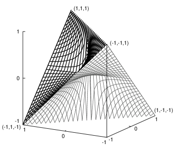
Figure 3: Graphical representation of the volume occupied by channels simulatable by a one-qubit mixed state environment. This volume is $\frac{3}{8}$ of the volume of the tetrahedron which represents all possible generalized depolarizing channels. All the vertices and edges of the tetrahedron are contained while no other point on any of the faces is contained.

Figure 4: Cross sections of the volume depicted in Figure 3 for different values of $z$ from $-1$ to $+1$. For each value of $z$ the rectangle is the cross section of the tetrahedron and the shaded area is the fraction simulatable with a one-qubit mixed state environment. The shaded fraction approaches zero as $|z|$ approaches $0$ and it approaches one as $|z|$ approaches $1$. In between for a given $z=z_{0}$ the darkened area is bounded by hyperbola $xy=z_{0}$ and lines $y=z_{0}x$ and $y=x/z_{0}$.

III.2 Two-Pauli channel

We now turn to an interesting sub-family of depolarizing channels, namely, the two-Pauli channel. Two-pauli channels are the ones for which only one of $\{\epsilon_{1},\epsilon_{2},\epsilon_{3}\}$ is zero and they are represented on the faces of the tetrahedron (leaving out the edges).

Further, for simplicity we restrict ourselves to a special case of a one-parameter sub-family of two-Pauli channels for which the nonzero elements are given by $\epsilon_{2}=0$ and $\epsilon_{1}=\epsilon_{2}=(1-\kappa)/2$ and $\epsilon_{0}=\kappa$. with $0\leq\kappa\leq 1$. The affine transformation for the two-Pauli channel can be easily computed and is given by

$$M^{\rm 2-Pauli}=\left(\begin{array}[]{lcr}\kappa\phantom{-1}&0&0\cr 0&\kappa&0\cr 0&0&2\kappa-1\end{array}\right)$$ (21)

This is a special case of the generalized depolarizing channels which is represented by a line on the face of the tetrahedron joining the vertex $(1,1,1)$ to the mid point of the edge below it. We take this particular case because it has been discussed in detail in the literature.

We will directly argue that the affine transformation (21) is not a special case of the affine transformation (19) for some values of $a$, $b$ and $c$. For the matrix (19) to take the form (21), two of its entries should become equal; let us assume that first two are equal. This forces $\cos a=\cos c$ and this further implies that $cosa$ is a factor of all the singular values. However, the affine transformation (21) does not have a non-trivial factor and hence the only possibility is $\cos a=1$. Now we impose the relationship between the equal and unequal singular values leading to $2\cos b-1=1$ which implies that $\cos b=1$. A similar result is obtained if we begin by equating any other pair of singular values in equation (19). The above analysis shows that the only place where the two-Pauli affine transformation can match the affine transformation (19) is when $\kappa=1$, at which point the two-Pauli channel disappears and one is left with the identity transformation. Thus we conclude that the two-Pauli channel is not a special case of (19). This result has been obtained earlier, where it was shown that the two-Pauli channel is a counter-example to the conjecture that a one-qubit mixed state environment can simulate all one-qubit quantum channels. Our demonstration is simpler and analytical, since we have obtained the explicit expression for the affine transformation. It is not difficult to generalize this argument for the other two-Pauli channels. Results about the points on the face of the tetrahedron not modelable using a one-qubit mixed state environment, are actually contained in the volume analysis of the previous section. We have presented the case of two-Pauli channels in detail due to the simplicity of the argument and the fact that two-Pauli channels have been discussed in the literature Terhal et al. (1999); Griffiths et al. (2006).

IV Concluding Remarks

We have obtained a canonical form corresponding to single qubit channels with a one-qubit mixed state modeling the environment. This parameterization has been obtained analytically by computing the affine transformation corresponding to this class of channels. Applying our results to the sub-class of depolarizing channels, we found that although a sizable volume ($\frac{3}{8}$ of the total volume) is modeled by a one-qubit mixed state environment, there is a finite volume in the channel space ($\frac{5}{8}$ of the total volume) which cannot be modeled in this fashion. The special case of the two-Pauli channel discussed in the literature has been shown to be in this missing volume and hence is not simulatable via a one-qubit mixed state environment. The results were achieved by starting with the general expression for the affine transformation, restricting it to the case with zero shift, and computing the singular values. It turns out that we can arrive at the precise constraints on the volume analytically, thereby producing a picture of the subset of generalized depolarizing channels simulatable by a one-qubit mixed state in the environment.

The affine transformation which we obtain is general and one can also explore channels other than the depolarizing channels. The analysis of the volume occupied by such channels in the entire channel space for one qubit is an involved problem and will be taken up elsewhere. We note that a similar conclusion about the two-Pauli channel from a very different perspective has been obtained in Griffiths et al. (2006).