Laser stabilization using spectral hole burning

Abstract

We have frequency stabilized a Coherent CR699-21 dye laser to a transient spectral hole on the 606 nm transition in Pr³⁺:Y₂SiO${}_{5}\,$. A frequency stability of 1 kHz has been obtained on the 10 µs timescale together with a long-term frequency drift below 1 kHz/s. RF magnetic fields are used to repopulate the hyperfine levels allowing us to control the dynamics of the spectral hole. A detailed theory of the atomic response to laser frequency errors has been developed which allows us to design and optimize the laser stabilization feedback loop, and specifically we give a stability criterion that must be fulfilled in order to obtain very low drift rates. The laser stability is sufficient for performing quantum gate experiments in Pr³⁺:Y₂SiO${}_{5}\,$.

I Introduction

Quantum information processing and the ability to experimentally manipulate quantum systems has evolved significantly over the past decade, and the search for new and potentially scalable qubit systems is ongoing. One of these schemes employs rare-earth-ion-doped crystals Ohlsson2002 ; Roos2004 ; Longdell2004 ; Longdell2004a ; Wesenberg2006 where, among others, the materials Pr³⁺:Y₂SiO${}_{5}\,$and Eu³⁺:Y₂SiO${}_{5}\,$are good candidates with very good coherence properties Equall1994 ; Equall1995 ; Fraval2004 ; Fraval2005 . Qubits are represented as hyperfine levels $\left|0\right>$ and $\left|1\right>$, and they are manipulated using an optical transition to an excited level $\left|\mathrm{e}\right>$. This optical manipulation requires very stable lasers in order to obtain high-fidelity gate operations. In order not to be limited by laser performance, the laser must remain phase coherent on a timescale comparable to the optical coherence time, $T_{2}$, of the atomic material. Our experimental focus is on Pr³⁺:Y₂SiO${}_{5}\,$which has an optical transition at 605.977 nm with coherence time as long as $T_{2}=152$ µs Equall1995 , which is accessible with dye lasers only. The narrow optical transitions are hidden inside a much broader inhomogeneous profile, but they can be isolated by optical pumping methods Nilsson2004 ; Rippe2005 , taking advantage of the very long hyperfine level lifetime (being $\approx$100 seconds in Pr³⁺:Y₂SiO${}_{5}\,$and much longer in a moderate magnetic field). These initialization techniques employ several cycles of population transfer with subsequent relaxation and may last for times of the order of several hundreds of milliseconds. This also places some long-term stability requirements on the laser performance.

Frequency stabilization of lasers is a science in itself. Previously, dye lasers have been stabilized using optical cavities Drever1983 ; Hough1984 ; Helmcke1987 ; Houssin1988 ; Kallenbach1989 ; Steiner1989 ; Zhu1992 ; Zhu1993 ; Sellars1995 ; Young1999 , and recently the method using spectral hole burning has been demonstrated with semi-conductor lasers Sellin1999 ; Strickland2000 ; Pryde2001 ; Pryde2002 ; Sellin2001 ; Bottger2001 ; Bottger2003 and with a Ti:sapphire laser Merkel2000 . We demonstrate for the first time a dye laser stabilized to a spectral hole. The method employing spectral holes has a number of advantages over optical cavities. Firstly, the sensitivity to vibrations requires that the atomic medium moves much less than an optical wavelength in an optical coherence time. However, for a high-finesse cavity this sensitivity is essentially multiplied by the average number of round trips made by a photon in the cavity, which can be several orders of magnitude. In addition, using the same hole-burning crystal for laser stabilization and for further experiments may reduce the sensitivity to vibrations significantly. Secondly, to make a phase-coherent laser on the timescale of $T_{2}$ requires a physical reference system with a phase memory of comparable duration. Hence, when performing experiments on e.g. Pr³⁺:Y₂SiO${}_{5}\,$, with $T_{2}=152$ µs, the material itself will automatically be sufficient for laser stabilization. A similar round trip time in a cavity is possible, but technically very challenging. A cavity also requires mode matching, and optical isolators are required to prevent the directly back-reflected field from entering the laser cavity. The main drawbacks of spectral holes include the requirement of cryogenic cooling, and for transient hole systems the long-term stability presents a challenge since the spectral hole position may change over time.

In the following sections we present a detailed theory of the dynamics of spectral holes and on the response of the atomic medium to errors in the laser frequency. This helped us to design the feedback hardware and in realizing the laser stabilization experimentally. In doing so, we also introduced an “RF-eraser”, which consists of RF magnetic fields controlling the hyperfine level lifetimes. In this manner, we can adjust and optimize the spectral hole dynamics for best laser performance. We also demonstrate experimental support for the theoretical calculations with emphasis on the problem of laser drift. The RF magnetic fields are very useful in this context. Apart from the theoretical understanding, it is also very important to build fast, low-noise, and low-offset feedback electronics. We have designed analog electronic circuits using the best components available on the market for the fastest parts of the regulation system. The most important design considerations are given in this paper, while the technical details are available elsewhere Rippe2006 ; GroupHomepage .

II Theoretical description of ion locking

The entire theoretical understanding of laser stabilization to spectral holes in inhomogeneous broadened transitions is one of the key results of this paper and is introduced in this section. Section II.1 presents simple arguments to explain the basic idea and to compare the procedure of locking to spectral holes with the method of locking to optical cavities. We then proceed to Secs. II.2 and II.3 where we introduce the Maxwell-Bloch equations, written in a form convenient for inhomogeneously broadened transitions and then calculate the propagation effects of laser light through the atomic material in the presence of spectral holes. With these results we are able to calculate the error signals suitable for the laser stabilization scheme using the Pound-Drever-Hall method Drever1983 in Sec. II.4. This section provides a general understanding of the response of atoms to errors in the laser frequency, which will put us in a position to design the electronics hardware for the stabilization feedback loop. In Sec. II.5 we analyze the possibility of linear drift errors and their prevention, and finally in Sec. II.6 we summarize our theoretical calculations.

The intention of this paper is to enable the reader to understand the details of laser stabilization to spectral holes with special emphasis on the feedback system design. Experimentally, we focus on a particular atomic system consisting of ions in a Pr³⁺:Y₂SiO${}_{5}\,$crystal. Instead of developing a general theory we make a few approximations suitable for this particular system. However, we present the calculations in such detail that it should be clear how to extend the theory to other systems.

In order to maintain the physical understanding we will restrict ourselves to analytical derivations and make approximations, rather than numerical simulations, when the calculations become difficult. Our theory is quantitatively accurate for many practical systems.

For readers not interested in all the technical details we will now summarize the most important theoretical results. After the simple discussion of laser stabilization schemes in Sec. II.1 we proceed to Sec. II.2 where we state in Eqs. (4-6) the important propagation equations for different frequency components of the laser light through matter. In Sec. II.3 these are applied to the special case of a spectral hole in a broad inhomogeneous profile in Eqs. (20) and (21) which, together with the hole shape parameters of Eqs. (14-16), form the workhorse for all calculations of error signals. In Sec. II.4 the error signals are calculated; the main result being the transfer function (36) connecting errors in laser frequency to modulations in the detected laser power. These calculations also indicate the optimum parameter choices for best performance. To mention one example, the modulation index $m=0.56$ in general optimizes the magnitude of the error signal which is different from the optimum result $m=1.08$ known from cavity locking Black2001 . However, additional constraints on the modulation index may be necessary when we take the possibility of laser drift into account in the rather technical section II.5. Here we calculate the correction (58) to the error signal if the laser is drifting linearly with time. This specifically leads to a criterion (59) which must be fulfilled in order to prevent laser drift. A practical version of this criterion is illustrated in Fig. 3.

II.1 Stabilization - an overview

Before entering into the detailed theoretical description of laser locking to spectral holes, we will give a general picture of the stabilization mechanisms. We discuss the concept of frequency locking and phase locking, and to this end we start by briefly discussing how stabilization to a cavity works. An extensive and pedagogical description can be found in Black2001 .

In stabilization setups with optical cavities the laser light is sent into a high-finesse cavity and the back-reflected light is detected. The aim is to maintain the laser frequency at the cavity resonance at all times, in which case the reflected field is ideally zero (all light is transmitted through the cavity). Let us assume that the cavity mirrors reflect 99.99% of the light intensity. The fact that no light is reflected in the ideal case is due to the fact that the immediately reflected laser field at the incoming mirror interferes destructively with the 0.01% leakage of the $10^{4}$ times more intense intra-cavity field.

Let us now assume that the incident light suddenly changes phase on a timescale much shorter than the cavity build-up time, $\tau=\frac{L}{Tc}$ (here $T=0.01\%$ is the mirror transmission, $c$ is the speed of light, and $L$ the cavity length. For $L=10$ cm we have $\tau\approx 3$ µs). The immediately reflected beam then changes its phase and does not interfere destructively with the cavity leakage field, which retains its original phase for a time of the order of $\tau$. The intensity is then non-zero and an error can be detected. The immediate phase difference (including the sign) of the two fields can be measured using the Pound-Drever-Hall method Drever1983 . If the phase change persists for a time longer than $\tau$ the reflected field returns to zero.

We also consider the case where the frequency is changed from the cavity resonance. On a timescale longer than $\tau$ this field will build up inside the cavity, but since the resonance condition is not met, the cavity length is not equal to an exact integer multiple of $\lambda/2$, where $\lambda$ is the wave length of the light. Hence, each round trip in the cavity is slightly advanced or delayed in phase, and the total contribution will be phase shifted, with a sign depending on the sign of the frequency error. When this field leaks out of the cavity and interferes with the immediately reflected field, we can again, in a similar fashion to above, measure the frequency error (including the sign). Note, that the non-zero reflection persists over time and is not limited to a duration $\tau$.

The above two examples illustrate the fact that on long timescales the detection and correction of frequency errors is possible, while phase errors can only be detected for a limited time given by the phase memory time $\tau$. We shall now argue that this picture also holds for locking to spectral holes. In this scenario the laser light is incident on an inhomogeneously broadened transition and the laser will burn a spectral hole in the absorbing background. To some extent, this spectral hole can be thought of as the inverse of the pedagogically simpler case with no background absorption and the presence of atoms at a single frequency only. We adopt this picture below.

It is well known that when scanning a laser across an atomic resonance the absorption will change (proportionally to $\frac{\Gamma_{\mathrm{h}}^{2}}{4}/(\frac{\Gamma_{\mathrm{h}}^{2}}{4}+\Delta^{2})$ where $\Gamma_{\mathrm{h}}$ is the full width half maximum (FWHM) line-width and $\Delta$ the detuning). At the same time, the index of refraction will change proportionally to $\Delta\frac{\Gamma_{\mathrm{h}}}{2}/(\frac{\Gamma_{\mathrm{h}}^{2}}{4}+\Delta^{2})$ which, for small detunings $\Delta$, causes a phase shift of the light proportional to the detuning. This effect can be detected by methods similar to the Pound-Drever-Hall method Drever1983 and is used for measuring frequency errors.

The above picture describes a steady state which requires modifications on short time scales. If the phase of the incoming light changes abruptly, it takes of the order of the optical coherence time $T_{2}=\frac{2}{\Gamma_{\mathrm{h}}}$ before the atoms have reached a new steady state ($\Gamma_{\mathrm{h}}$ is here measured in rad/sec). Meanwhile, the atoms keep radiating at the original phase, which allows the phase error to be measured but only for a limited time, $T_{2}$.

We see that the methods of optical cavities and spectral holes are very similar. In a common picture we can think of both as frequency filters where the phase memory is set by the inverse line-width and the filtering gives rise to slowly varying fields. The possibility of detecting phase errors relies on the interference between an immediately changing field and the slowly varying field. For the optical cavity the immediately changing field is the directly reflected beam, while for spectral holes it is the remaining part of the incoming light transmitted through the atoms. The slowly varying field is the intra-cavity field in the case of optical cavities, while it is the light emitted coherently by atoms in the case of spectral holes. The Pound-Drever-Hall method Drever1983 allows for the detection of the above mentioned interference in both cases, but there is one important difference. The modulation sidebands required for this scheme are not stored in the optical cavity (they are not resonant) and hence do not experience the frequency filtering. For the method of spectral holes these sidebands create side holes which must be taken into account to understand the complete picture.

II.2 Two-level atoms and Maxwell-Bloch equations

For the detailed theoretical calculations we start with an ensemble of inhomogeneously broadened two-level atoms. We allow laser light to propagate through these along the $z$-direction. With a large beam cross section a one-dimensional theory is sufficient, and the Maxwell-Bloch equations can be written (see e.g. Allen1975 ; Milonni1988 ; Mandel1995 ):

$$\frac{\partial}{\partial t}(u-iv)=-(\frac{\Gamma_{\mathrm{h}}}{2}+i\Delta)(u-iv)-i\Omega w,$$ (1)

$$\frac{\partial}{\partial t}w=\frac{i}{2}\left[\Omega(u+iv)-\Omega^{*}(u-iv)\right]-\frac{1}{T_{1}}(1+w),$$ (2)

$$\left(\frac{\partial}{\partial z}+\frac{n}{c}\frac{\partial}{\partial t}\right)\Omega=\frac{i\alpha_{0}}{2\pi}\int_{-\infty}^{\infty}g(\Delta)(u-iv)d\Delta.$$ (3)

Here $(u,v,w)$ is the usual Bloch-vector which depends on time $t$, position $z$, and detuning $\Delta$ (from a chosen reference point). The electric field is described in terms of the complex Rabi frequency $\Omega(z,t)=\mu\mathcal{E}(z,t)/\hbar$, where $\mathcal{E}$ is the complex electric field and $\mu$ is the dipole moment along the direction of the field (we consider only a single linear polarization mode). $\Gamma_{\mathrm{h}}=2/T_{2}$ is the FWHM homogeneous line-width of the atoms in rad/sec, $T_{1}$ and $T_{2}$ are the life and coherence times of the optical transition, respectively. In Eq. (3) $n$ is the refractive index of non-absorbing background atoms, and $g(\Delta)$ is a dimensionless function describing the inhomogeneous distribution of atoms such that $g(\Delta)$ is proportional to the number of atoms with transition frequency $\Delta$. We use an unconventional but experimentally convenient normalization such that if the absorption length measured with a weak laser field at frequency $\Delta_{0}$ amounts to $\alpha_{0}$, then $g(\Delta_{0})$ must be unity. The integral over $\Delta$ in Eq. (3) effectively adds the contribution of the polarization from all the atoms to the electric field $\Omega$ at position $z$ and time $t$.

Eqs. (1-3) are in general difficult to solve analytically. However, for our specific needs regarding laser stabilization we will make a number of approximations in the following. We start by noting that in Eq. (3) the term $\frac{n}{c}\frac{\partial\Omega}{\partial t}$ is only relevant when describing very fast changes, on the time scale $L/c$ where $L$ is the length of the sample. We therefore neglect this term completely.

II.2.1 Linear regime of Maxwell-Bloch equations

The next approximation is to consider Eqs. (1-3) in the linear regime where, $w\approx-1$ for all atoms, i.e. the probability of being in the excited state is small. In Sec. II.3 we discuss the validity of this approximation. Inserting (with $w=-1$) the integral form $u(z,t)-iv(z,t)=i\int_{-\infty}^{t}e^{-(\frac{\Gamma_{\mathrm{h}}}{2}+i\Delta)(t-t^{\prime})}\Omega(z,t^{\prime})dt^{\prime}$ of Eq. (1) into Eq. (3) and expressing the electric field $\Omega$ in terms of its Fourier components, $\Omega(z,t)=\int_{-\infty}^{\infty}\Omega(z,\omega)e^{-i\omega t}d\omega$, it follows that Eq. (3) can be written in Fourier space as:

$$\begin{split}\frac{\partial}{\partial z}\Omega(z,\omega)&=-\frac{\alpha_{0}}{2\pi}\int_{-\infty}^{\infty}\frac{g(\Delta)d\Delta}{\frac{\Gamma_{\mathrm{h}}}{2}+i(\Delta-\omega)}\Omega(z,\omega)\\ &\equiv-\frac{\alpha_{\mathrm{R}}(\omega)+i\alpha_{\mathrm{I}}(\omega)}{2}\Omega(z,\omega).\end{split}$$ (4)

where we define $\alpha_{\mathrm{R}}(\omega)$ and $\alpha_{\mathrm{I}}(\omega)$ as the real and imaginary absorption lengths, respectively. For a single frequency component of the field $\Omega(z,\omega)=A(z,\omega)e^{-i\phi(z,\omega)}$ with real amplitude $A$ and phase $\phi$ we have the relation:

$$\frac{\partial A(z,\omega)}{\partial z} =-\frac{\alpha_{\mathrm{R}}(\omega)}{2}A(z,\omega),$$ (5)

$$\frac{\partial\phi(z,\omega)}{\partial z} =+\frac{\alpha_{\mathrm{I}}(\omega)}{2}.$$ (6)

Eqs. (4-6) will be the workhorse for many calculations in the following sections. Our goal is to model the frequency variations of the incoming laser field, propagate this field through the atomic medium via Eqs. (5) and (6), and finally derive an error signal useful for frequency stabilization based on the outgoing field. We will reach this goal in Sec. II.4, but before that we introduce a model which describes the effect of hole burning in terms of the shape function, $g(\Delta)$.

II.2.2 Example: Inhomogeneous profiles

Let us give a simple and useful example of the above equations. Consider a Lorentzian-shaped inhomogeneous profile, $g(\Delta)=\frac{\Gamma_{\mathrm{inh}}^{2}}{4}/\left(\frac{\Gamma_{\mathrm{inh}}^{2}}{4}+\Delta^{2}\right)$. Using the residue theorem we find (for $\Gamma_{\mathrm{inh}}\gg\Gamma_{\mathrm{h}}$):

$$\alpha_{\mathrm{R}}(\omega)=\alpha_{0}\frac{\frac{\Gamma_{\mathrm{inh}}^{2}}{4}}{\frac{\Gamma_{\mathrm{inh}}^{2}}{4}+\omega^{2}},\quad\alpha_{\mathrm{I}}(\omega)=\alpha_{0}\frac{\omega\frac{\Gamma_{\mathrm{inh}}}{2}}{\frac{\Gamma_{\mathrm{inh}}^{2}}{4}+\omega^{2}}.$$ (7)

Here we have chosen the frequency zero point to be at the center of the profile. We see that the absorption length at this frequency is $\alpha_{0}$, consistent with $g(\Delta)=1$ for $\Delta=0$.

We could also consider a Gaussian-shaped profile, $g(\Delta)=\exp\left(-4\ln(2)\Delta^{2}/\Gamma_{\mathrm{inh}}^{2}\right)$, with FWHM $\Gamma_{\mathrm{inh}}$. Inserting this into Eq. (4) we find with help from Abramowitz1972 , $\frac{\partial\Omega(z,\omega)}{\partial z}=-\frac{\alpha_{0}w(Z)}{2}\Omega(z,\omega)$, where $Z=\frac{2\sqrt{\ln 2}}{\Gamma_{\mathrm{inh}}}(\omega+i\frac{\Gamma_{\mathrm{h}}}{2})$ and $w(Z)$ is the error function for complex arguments. Thus $\alpha_{\mathrm{R}}=\alpha_{0}\mathrm{Re}\{w(Z)\}$ and $\alpha_{\mathrm{I}}=\alpha_{0}\mathrm{Im}\{w(Z)\}$, known as the Voigt profile Milonni1988 . In general, the shape of the inhomogeneous profile varies depending on the broadening mechanism Stoneham1969 ; Wesenberg2004d .

II.3 Two-level atoms with a reservoir state

The calculations in the previous sections need to be refined in order to describe the effect of spectral hole burning. So, in addition to the ground $\left|\mathrm{g}\right>$ and excited $\left|\mathrm{e}\right>$ states we add a third reservoir state $\left|\mathrm{r}\right>$ (see Fig. 4(b)) and write the Bloch equations for these:

$$\frac{\partial}{\partial t}(u-iv) =-(\frac{\Gamma_{\mathrm{h}}}{2}+i\Delta)(u-iv)-i\Omega(\rho_{e}-\rho_{g}),$$ (8)

$$\frac{\partial\rho_{e}}{\partial t} =\frac{i}{4}\left[\Omega(u+iv)-\Omega^{*}(u-iv)\right]-\frac{1}{T_{1}}\rho_{e},$$ (9)

$$\frac{\partial\rho_{g}}{\partial t} =-\frac{i}{4}\left[\Omega(u+iv)-\Omega^{*}(u-iv)\right]$$

$$\quad+\frac{b_{\mathrm{eg}}}{T_{1}}\rho_{e}-\frac{1}{T_{\mathrm{gr}}}\rho_{g}+\frac{1}{T_{\mathrm{rg}}}\rho_{r},$$ (10)

$$\frac{\partial\rho_{r}}{\partial t} =\frac{b_{\mathrm{er}}}{T_{1}}\rho_{e}+\frac{1}{T_{\mathrm{gr}}}\rho_{g}-\frac{1}{T_{\mathrm{rg}}}\rho_{r}.$$ (11)

We assume the optical field, $\Omega$, only couples to the transition $\left|\mathrm{g}\right>\rightarrow\left|\mathrm{e}\right>$ and hence $u$ and $v$ still refer to this transition, and only the factor $w=\rho_{\mathrm{e}}-\rho_{\mathrm{g}}$ appears in the driving term in Eq. (8), as was the case in Eq. (1). We add the possibility of decays from the excited state to the reservoir state. The branching ratios from $\left|\mathrm{e}\right>$ to $\left|\mathrm{g}\right>$ and $\left|\mathrm{e}\right>$ to $\left|\mathrm{r}\right>$ are denoted $b_{\mathrm{eg}}$ and $b_{\mathrm{er}}$, respectively. We also model relaxation between the $\left|\mathrm{g}\right>$ and $\left|\mathrm{r}\right>$ levels. The timescale for decays from $\left|\mathrm{g}\right>$ to $\left|\mathrm{r}\right>$ is $T_{\mathrm{gr}}$, which in general need not be the same as the timescale $T_{\mathrm{rg}}$ in the opposite direction. For the homogeneous line-width, $\Gamma_{\mathrm{h}}$, we now have:

$$\frac{\Gamma_{\mathrm{h}}}{2}=\frac{1}{T_{2}}=\frac{1}{T_{2}^{(0)}}+\frac{1}{2T_{\mathrm{gr}}},$$ (12)

where $T_{2}^{(0)}$ is the coherence time of the optical transition $\left|\mathrm{g}\right>\rightarrow\left|\mathrm{e}\right>$ in the absence of ground state relaxation, and the term $\frac{1}{2T_{\mathrm{gr}}}$ takes the finite lifetime of the state $\left|\mathrm{g}\right>$ into account.

II.3.1 Separation of timescales

Our next step from Eqs. (8-11) is to use steady-state solutions for $\rho_{\mathrm{e}}$, $\rho_{\mathrm{g}}$, and $\rho_{\mathrm{r}}$ while $u$ and $v$ still are allowed to vary in time according to Eq. (8). This is a good approximation since in our specific case we have naturally different timescales for the ground state populations and the optical coherence, $T_{\mathrm{rg}},T_{\mathrm{gr}}\gg T_{2}$. Furthermore, when the laser is actively stabilized to a line-width narrower than $\Gamma_{\mathrm{h}}$, it is a good approximation to assume a zeroth order starting point, $\Omega=\Omega_{0}e^{-i\Delta_{0}t}$, where the laser is running perfectly at a monochromatic frequency, $\Delta_{0}$. If the variations from this starting point are small, the populations will always be close to their steady-state values.

So, with $\Omega=\Omega_{0}e^{-i\Delta_{0}t}$ we calculate the steady-state solutions of Eqs. (8-11). With a little work we obtain and expression for the population difference $\rho_{\mathrm{g}}-\rho_{\mathrm{e}}$ ($\rho_{\mathrm{e}}$, $\rho_{\mathrm{g}}$, and $\rho_{\mathrm{r}}$ are given in detail in Eq. (54)):

$$\rho_{\mathrm{g}}-\rho_{\mathrm{e}}=G\left(1-d_{\mathrm{hole}}\frac{\frac{\Gamma_{\mathrm{hole}}^{2}}{4}}{\frac{\Gamma_{\mathrm{hole}}^{2}}{4}+(\Delta-\Delta_{0})^{2}}\right),$$ (13)

where $d_{\mathrm{hole}}$ is the relative hole depth and $\Gamma_{\mathrm{hole}}$ is the FWHM of the hole. These parameters can be written:

$$d_{\mathrm{hole}}=\frac{(1+R)\frac{s_{0}}{2}}{1+(1+R)\frac{s_{0}}{2}},\quad\Gamma_{\mathrm{hole}}=\Gamma_{\mathrm{h}}\sqrt{1+(1+R)\frac{s_{0}}{2}},$$ (14)

where $s_{0}$ is the resonant saturation parameter:

$$s_{0}=|\Omega_{0}|^{2}T_{1}T_{2},$$ (15)

and for our particular case of Eqs. (8-11) we have:

$$R=\frac{1+\frac{b_{\mathrm{er}}T_{\mathrm{rg}}}{T_{1}}}{1+\frac{T_{\mathrm{rg}}}{T_{\mathrm{gr}}}},\quad G=\frac{1}{1+\frac{T_{\mathrm{rg}}}{T_{\mathrm{gr}}}}.$$ (16)

The saturation parameter $s_{0}$ is a measure of the probability of an atom being in the excited state $\left|\mathrm{e}\right>$ at resonance. In steady state at $\Delta=\Delta_{0}$ we have $\frac{\rho_{\mathrm{e}}}{\rho_{\mathrm{g}}}=\frac{s_{0}}{2}/\left(1+\frac{s_{0}}{2}\right)$. The parameter $G$ is a measure of the fraction of atoms in the ground state $\left|\mathrm{g}\right>$ in equilibrium in the absence of the laser light or when the detuning, $\Delta-\Delta_{0}$, is large. The parameter $R$ is a measure of how likely it is for an atom to be trapped in the reservoir state. The essence of $R$ is in the term $b_{\mathrm{er}}T_{\mathrm{rg}}/T_{1}$, which is the ratio of the rate $b_{\mathrm{er}}/T_{1}$ from $\left|\mathrm{e}\right>$ into the reservoir state $\left|\mathrm{r}\right>$ and the rate $1/T_{\mathrm{rg}}$ out of the reservoir state. From Eq. (14) it is clear that a spectral hole can be deep and broad for different reasons: Firstly, if the laser field is strong with a high saturation parameter $s_{0}$, although $R$ is small, and secondly, if the trapping parameter $R$ is large even a weak field with $s_{0}\ll 1$ is capable of digging a deep, wide hole.

Now, we wish to employ Eq. (3) or (4) together with Eqs. (8-11). We insert the steady-state value of Eq. (13) into Eq. (8) written in integral form. Since the steady-state value is time-independent we may perform the same steps as those leading to Eq. (4). We will incorporate the value of $\rho_{\mathrm{g}}-\rho_{\mathrm{e}}$ into the $g(\Delta)$ shape function and just pretend that we never left the linear approximation, Eq. (4), of a two-level system. This is done correctly when:

$$g(\Delta)=\frac{\rho_{\mathrm{g}}-\rho_{\mathrm{e}}}{G}=1-\frac{d_{\mathrm{hole}}\frac{\Gamma_{\mathrm{hole}}^{2}}{4}}{\frac{\Gamma_{\mathrm{hole}}^{2}}{4}+(\Delta-\Delta_{0})^{2}}.$$ (17)

The division by $G$ (the fraction of atoms in $\left|\mathrm{g}\right>$ far off resonance) assures that $g(\Delta)$ is correctly normalized to unity away from the spectral hole, i.e. $\alpha_{0}$ is the absorption length for a weak laser field in the absence of the spectral hole.

Let us retrace our steps so far and underline the approximations made. We have reached the two important equations (4) and (17). The $g(\Delta)$ function for a spectral hole describes how many atoms actually participate in the active two-level transition $\left|\mathrm{g}\right>\rightarrow\left|\mathrm{e}\right>$. We included the effect of saturation where atoms can also populate the excited state $\left|\mathrm{e}\right>$ (which mathematically also creates a hole in $\rho_{\mathrm{g}}-\rho_{\mathrm{e}}$). However, since we assumed the populations $\rho_{\mathrm{e}}$, $\rho_{\mathrm{g}}$, and $\rho_{\mathrm{r}}$ to be essentially constant in time, we have restricted ourselves to solutions where the laser field does not deviate much from a perfect field, $\Omega=\Omega_{0}e^{-i\Delta_{0}t}$ (we have linearized the theory around this zeroth order solution). Note, that the field $\Omega$ can still have fast variations in e.g. its phase, as long as the phase excursions are not too large. Since both population trapping in the reservoir state and the effect of saturation (leading to population trapping in the excited state) are incorporated into the single parameter $g(\Delta)$, we effectively model the three-level equations (8-11) with our initial linear two-level system with low saturation, as described by Eq. (4).

Using Eq. (17) also requires another approximation. We note that $d_{\mathrm{hole}}$ and $\Gamma_{\mathrm{hole}}$ depend on the resonant saturation parameter, $s_{0}$. If the optical depth, $\alpha_{0}L$, of the atomic sample is large, the saturation parameter will depend on $z$, and the use of a $z$-independent $g(\Delta)$ will be incorrect. However, if the laser field burns holes, the attenuation will be less than $\alpha_{0}L$. Practically, the equations will be applicable for $\alpha_{0}L$ not too much greater than unity.

Finally, we point out that $d_{\mathrm{hole}}$ and $\Gamma_{\mathrm{hole}}$, as defined in Eq. (14), refer to the structure in the population, not to the depth and width which would be measured in an absorption experiment. From (14) we always have the relation:

$$1-d_{\mathrm{hole}}=\left(\frac{\Gamma_{\mathrm{h}}}{\Gamma_{\mathrm{hole}}}\right)^{2}.$$ (18)

II.3.2 Absorption and phase shift from a spectral hole

Let us now employ Eqs. (4) and (17) to calculate the attenuation and phase shift of a laser field in the presence of a spectral hole. We take for the $g(\Delta)$ function:

$$g(\Delta)=\frac{\frac{\Gamma_{\mathrm{inh}}^{2}}{4}}{\frac{\Gamma_{\mathrm{inh}}^{2}}{4}+\Delta^{2}}\left(1-\frac{d_{\mathrm{hole}}\frac{\Gamma_{\mathrm{hole}}^{2}}{4}}{\frac{\Gamma_{\mathrm{hole}}^{2}}{4}+(\Delta-\Delta_{0})^{2}}\right),$$ (19)

i.e. we have a spectral hole burned at frequency $\Delta_{0}$ into an inhomogeneously broadened Lorentzian profile with width $\Gamma_{\mathrm{inh}}$ centered at $\Delta=0$. Inserting this into Eq. (4) we find, with the help from the residue theorem,

$$\alpha_{\mathrm{R}}(\omega) =\alpha_{0}\left[\frac{\frac{\Gamma_{\mathrm{inh}}^{2}}{4}}{\frac{\Gamma_{\mathrm{inh}}^{2}}{4}+\omega^{2}}-\frac{\frac{\Gamma_{\mathrm{inh}}^{2}}{4}}{\frac{\Gamma_{\mathrm{inh}}^{2}}{4}+\Delta_{0}^{2}}\cdot\frac{\frac{\Gamma_{\mathrm{hole}}(\Gamma_{\mathrm{hole}}+\Gamma_{\mathrm{h}})}{4}d_{\mathrm{hole}}}{\frac{(\Gamma_{\mathrm{hole}}+\Gamma_{\mathrm{h}})^{2}}{4}+(\Delta_{0}-\omega)^{2}}\right]\rightarrow\alpha_{0}\left[1-\frac{\frac{\Gamma_{\mathrm{hole}}(\Gamma_{\mathrm{hole}}+\Gamma_{\mathrm{h}})}{4}d_{\mathrm{hole}}}{\frac{(\Gamma_{\mathrm{hole}}+\Gamma_{\mathrm{h}})^{2}}{4}+(\Delta_{0}-\omega)^{2}}\right],$$ (20)

$$\alpha_{\mathrm{I}}(\omega) =\alpha_{0}\left[\frac{\omega\frac{\Gamma_{\mathrm{inh}}}{2}}{\frac{\Gamma_{\mathrm{inh}}^{2}}{4}+\omega^{2}}+\frac{\frac{\Gamma_{\mathrm{inh}}^{2}}{4}}{\frac{\Gamma_{\mathrm{inh}}^{2}}{4}+\Delta_{0}^{2}}\cdot\frac{\frac{\Gamma_{\mathrm{hole}}}{2}(\Delta_{0}-\omega)d_{\mathrm{hole}}}{\frac{(\Gamma_{\mathrm{hole}}+\Gamma_{\mathrm{h}})^{2}}{4}+(\Delta_{0}-\omega)^{2}}\right]\rightarrow\alpha_{0}\frac{\frac{\Gamma_{\mathrm{hole}}}{2}(\Delta_{0}-\omega)d_{\mathrm{hole}}}{\frac{(\Gamma_{\mathrm{hole}}+\Gamma_{\mathrm{h}})^{2}}{4}+(\Delta_{0}-\omega)^{2}},$$ (21)

with $\Gamma_{\mathrm{hole}}$ and $d_{\mathrm{hole}}$ defined in Eq. (14). In the first terms we assumed that $\Gamma_{\mathrm{inh}}\gg\Gamma_{\mathrm{h}}$. The arrows indicate the limit when $\Gamma_{\mathrm{inh}}\rightarrow\infty$, i.e. when we neglect the effect of the possibly very wide inhomogeneous background. Note, we had to include the inhomogeneous profile in this calculation since otherwise $g(\Delta)\rightarrow 1$ for $\Delta\rightarrow\infty$, making the integral in Eq. (4) divergent. Note, also that the factors containing $\Gamma_{\mathrm{inh}}$ are given by Eq. (7) and they may be replaced by the corresponding results for a Gaussian profile.

If we compare Eqs. (17) and (20) we see that in an absorption measurement with a weak field (not changing the populations further) the measured width and depth of the hole are related to $\Gamma_{\mathrm{hole}}$ and $d_{\mathrm{hole}}$ by:

$$\Gamma_{\mathrm{hole}}^{\mathrm{(meas)}}=\Gamma_{\mathrm{hole}}+\Gamma_{\mathrm{h}},\quad d_{\mathrm{hole}}^{\mathrm{(meas)}}=\frac{\Gamma_{\mathrm{hole}}d_{\mathrm{hole}}}{\Gamma_{\mathrm{hole}}+\Gamma_{\mathrm{h}}}.$$ (22)

II.4 Calculation of error signals

Now, let us turn to the calculation of real error signals used in the locking procedure. We will start simply by connecting the Rabi frequency, $\Omega$, used in the theoretical calculations, with real experimental parameters, and we will also state the well known results from Pound-Drever-Hall frequency modulation Drever1983 ; Bjorklund1983 .

To this end, we assume the laser field propagating into the locking system is perfectly monochromatic, with $E^{(\mathrm{in})}(t)=\mathrm{Re}\{\mathcal{E}_{0}e^{-i\Delta_{0}t}\}$ in the rotating frame. The electric field is connected to the incoming intensity through the relation $I^{(\mathrm{in})}=|\mathcal{E}_{0}|^{2}/2\mu_{0}c$, which again is connected to the incoming power, $P$, and cross-sectional area $A$ by $I^{(\mathrm{in})}=P^{(\mathrm{in})}/A$. Since we have defined the Rabi frequency as $\Omega=\mu\mathcal{E}/\hbar$, where $\mathcal{E}$ is the complex electric field inside the atomic sample, we can equivalently describe our monochromatic incoming laser field in terms of the complex Rabi frequency:

$$\Omega(0,t)=\Omega_{0}e^{-i\Delta_{0}t}\quad\text{with }\Omega_{0}=\frac{\mu}{\hbar}\sqrt{\frac{2\mu_{0}cP}{nA}}.$$ (23)

Here the refractive index $n$ takes into account the fact that the electric field is different inside and outside the atomic sample.

Next, we phase modulate this incoming laser field at frequency $\omega_{\mathrm{m}}$ such that:

$$\begin{split}\Omega(0,t)&=\Omega_{0}e^{-i[\Delta_{0}t+m\sin(\omega_{\mathrm{m}}t)]}\\ &\approx\Omega_{0}(J_{0}+J_{1}e^{-i\omega_{\mathrm{m}}t}-J_{1}e^{i\omega_{\mathrm{m}}t})e^{-i\Delta_{0}t},\end{split}$$ (24)

where $m$ is the modulation index, which is assumed to be small in the second line, such that only the first sideband is significant. $J_{0}$ and $J_{1}$ are the Bessel functions of the first kind with $m$ as the argument.

It is now time to pass this modulated field through the atomic sample. We shall simply assume that for the carrier, upper sideband, and lower sideband, respectively, there are constant phase shifts of $\phi_{\mathrm{c}}$, $\phi_{+}$, and $\phi_{-}$ and constant transmission coefficients $\eta_{\mathrm{c}}$, $\eta_{+}$, and $\eta_{-}$ of the amplitudes, such that the outgoing Rabi frequency can be written:

$$\begin{split}\Omega(L,t)=\Omega_{0}\{&\eta_{\mathrm{c}}J_{0}e^{-i\phi_{\mathrm{c}}}+\eta_{+}J_{1}e^{-i(\omega_{\mathrm{m}}t+\phi_{+})}\\ -&\eta_{-}J_{1}e^{i(\omega_{\mathrm{m}}t-\phi_{-})}\}e^{-i\Delta_{0}t}.\end{split}$$ (25)

These $\eta$ and $\phi$ parameters may be calculated from Eqs. (20) and (21). When the above field hits a photo-detector, they will generate a photo-current proportional to the power $P^{(\mathrm{out})}(t)$ incident on the detector. This power is time-dependent and can be calculated from the above equation together with the absolute square of Eq. (23) to give:

$$\begin{split}P^{(\mathrm{out})}(t)=P^{(\mathrm{in})}&\left\{\left[J_{0}^{2}\eta_{\mathrm{c}}^{2}+J_{1}^{2}(\eta_{+}^{2}+\eta_{-}^{2})\right]+J_{0}J_{1}\eta_{\mathrm{c}}\left[(\eta_{+}+\eta_{-})\sin\left(\phi_{\mathrm{c}}-\frac{\phi_{+}+\phi_{-}}{2}\right)\sin\left(\omega_{\mathrm{m}}t+\frac{\phi_{+}-\phi_{-}}{2}\right)\right.\right.\\ &\qquad\qquad\qquad\qquad\qquad\qquad\qquad+\!\left.\left.(\eta_{+}-\eta_{-})\cos\left(\phi_{\mathrm{c}}-\frac{\phi_{+}+\phi_{-}}{2}\right)\cos\left(\omega_{\mathrm{m}}t+\frac{\phi_{+}-\phi_{-}}{2}\right)\right]\right\}.\end{split}$$ (26)

It takes some trigonometric relations to reach this, and we have neglected the higher order contribution oscillating at $2\omega_{\mathrm{m}}$.

The first term in square brackets is a DC term describing the average power reaching the detector. The second term in square brackets is that useful and important for laser stabilization and closely resembles the well known result from Bjorklund1983 . Here, this term is not expressed in the most useful form for calculations, but it clarifies some important qualitative properties of the error signal at different demodulation phases for our particular setup.

First of all, the term $\frac{\phi_{+}-\phi_{-}}{2}$ is always rather small. For a broad inhomogeneous profile ($\Gamma_{\mathrm{inh}}\gg\omega_{\mathrm{m}}$) in the absence of hole burning the phase changes little for a frequency variation of $\omega_{\mathrm{m}}$, and the phase difference $\phi_{+}-\phi_{-}$ is small. In the presence of a spectral hole the phase may change dramatically with small frequency changes, but the two side holes at frequencies $\Delta_{0}\pm\omega_{\mathrm{m}}$ are almost identical and the phase difference remains small. In any case, we always have $\frac{\phi_{+}-\phi_{-}}{2}\lesssim\alpha_{0}L\omega_{\mathrm{m}}/\Gamma_{\mathrm{inh}}\ll 1$ (unless $\alpha_{0}L$ is ridiculously large). As a result, we need only consider the two terms in the rightmost square brackets above to be pure sine and cosine terms, respectively. Note, some work has been performed on narrow inhomogeneous profiles in the case when $\Gamma_{\mathrm{inh}}\gg\omega_{\mathrm{m}}$ does not hold Bottger2007 .

Secondly, the term $\phi_{\mathrm{c}}-\frac{\phi_{+}+\phi_{-}}{2}$ depends strongly on the situation. If the atomic contribution to the phase varies slowly versus frequency on a scale broader than $\omega_{\mathrm{m}}$, this terms is small. For instance, for an inhomogeneously broadened profile with width $\Gamma_{\mathrm{inh}}$ and no hole-burning effects, we must have $\phi_{\mathrm{c}}-\frac{\phi_{+}+\phi_{-}}{2}=O([\omega_{\mathrm{m}}/\Gamma_{\mathrm{inh}}]^{2})$, since $\phi_{\mathrm{c}}=\frac{\phi_{+}+\phi_{-}}{2}$ to first order. In this case the $\sin(\omega_{\mathrm{m}}t)$-term in Eq. (26) is second order in $\omega_{\mathrm{m}}/\Gamma_{\mathrm{inh}}$. At the same time, we have in general that $\eta_{+}-\eta_{-}$ varies to first order in $\omega_{\mathrm{m}}/\Gamma_{\mathrm{inh}}$, while $\cos(\phi_{\mathrm{c}}-\frac{\phi_{+}+\phi_{-}}{2})\approx 1$. Hence the $\cos(\omega_{\mathrm{m}}t)$ term is much larger than the $\sin(\omega_{\mathrm{m}}t)$ term, which can be neglected.

The situation changes when hole burning is present. Then, in general, the difference between $\phi_{\mathrm{c}}$ and $\phi_{\pm}$ can be quite large, and both $\cos(\phi_{\mathrm{c}}-\frac{\phi_{+}+\phi_{-}}{2})$ and $\sin(\phi_{\mathrm{c}}-\frac{\phi_{+}+\phi_{-}}{2})$ can be on the order of unity. At the same time, $\eta_{+}+\eta_{-}$ can be on the order of unity while $\eta_{+}-\eta_{-}$ is of the order of $\omega_{\mathrm{m}}/\Gamma_{\mathrm{inh}}$. Hence the $\sin(\omega_{\mathrm{m}}t)$ term is on the order of unity and dominates the weaker $\cos(\omega_{\mathrm{m}}t)$ term.

Experimentally, we may demodulate the signal given by Eq. (26) by mixing it with a local oscillator in order to obtain a useful error signal for the laser stabilization system. When choosing the phase in this procedure there may be unknown phase shifts in amplifiers, etc., but the “cosine” or “sine” quadrature can be found by maximizing or minimizing the error signal when hole burning is not present (for rare-earth-ion-doped crystals this can be done at an elevated temperature).

II.4.1 Harmonic analysis

Above we have calculated the detected power in a case when the input light is perfectly monochromatic. In reality the input light will vary in amplitude and frequency over time. The amplitude variations are relatively easy to measure and correct for; we briefly discuss how we do this experimentally in Sec. III.1. Hence, in the following we concentrate on frequency errors. We may imagine that the transmission coefficients $\eta_{\mathrm{c}}$, $\eta_{+}$, and $\eta_{-}$ and phase shifts $\phi_{\mathrm{c}}$, $\phi_{+}$, and $\phi_{-}$ in Eq. (26) vary in time, which calls for further calculations. In general, a convenient method is to assume the incoming laser field to be of the form:

$$\Omega(0,t)=\Omega_{0}e^{-i(\Delta_{0}t+\epsilon\sin(\omega t))},$$ (27)

i.e. we have an almost single-frequency laser at $\Delta_{0}$, but with an additional small harmonic disturbance of the phase with frequency $\omega$ and magnitude $\epsilon$, which we assume to be much less than unity. We note that the instantaneous laser frequency, $\omega^{\mathrm{inst}}_{0}$, is then given by:

$$\omega^{\mathrm{inst}}_{0}=\frac{\partial\phi(t)}{\partial t}=\Delta_{0}+\epsilon\omega\cos(\omega t).$$ (28)

The above model is valid when the laser is running in the frequency stabilized mode with a narrow line-width. After phase modulating the beam at frequency $\omega_{\mathrm{m}}$ the light field becomes:

$$\begin{split}\Omega(0,t)&\approx\Omega_{0}(1+\frac{\epsilon}{2}e^{-i\omega t}-\frac{\epsilon}{2}e^{i\omega t})\\ &\quad\times(J_{0}+J_{1}e^{-i\omega_{\mathrm{m}}t}-J_{1}e^{i\omega_{\mathrm{m}}t})e^{-i\Delta_{0}t},\end{split}$$ (29)

which is just Eq. (24) together with the harmonic error of Eq. (27) for $\epsilon\ll 1$.

We now have nine frequency components which will propagate through our atomic medium, and we will treat these in a similar manner as in Eq. (25). To this end we make the following assumptions. Since $\epsilon$ is small there is so little energy in the $\omega$-sidebands that these have no hole-burning effects. Consequently, we will have three spectral holes at frequencies $\Delta_{0}$ and $\Delta_{0}\pm\omega_{\mathrm{m}}$. For these holes we have $\Gamma_{\mathrm{hole}}\ll\omega_{\mathrm{m}}$ such that the holes can be treated independently when utilizing Eqs. (20) and (21). We also neglect the effect of the inhomogeneous profile ($\Gamma_{\mathrm{inh}}\gg\omega_{\mathrm{m}}$). As a consequence, the two spectral holes at frequencies $\Delta_{0}\pm\omega_{\mathrm{m}}$ become identical and we introduce a common absorption coefficient, $\eta_{\mathrm{s}}=\eta_{+}=\eta_{-}$ and phase shift, $\phi_{\mathrm{s}}=\phi_{+}=\phi_{-}$ where “s” refers to the sidebands at frequency $\omega_{\mathrm{m}}$.

Introducing the hole widths $\Gamma_{\mathrm{hole,c}}$, $\Gamma_{\mathrm{hole,s}}$ and hole depths $d_{\mathrm{hole,c}}$, $d_{\mathrm{hole,s}}$ for the carrier and sidebands, respectively, we may define:

$$\eta_{i}(\omega) =\exp\left(-\frac{\alpha_{0}L}{2}\left[1-\frac{\frac{\Gamma_{\mathrm{hole},i}(\Gamma_{\mathrm{hole},i}+\Gamma_{\mathrm{h}})}{4}d_{\mathrm{hole},i}}{\frac{(\Gamma_{\mathrm{hole},i}+\Gamma_{\mathrm{h}})^{2}}{4}+\omega^{2}}\right]\right),$$ (30)

$$\phi_{i}(\omega) =-\frac{\alpha_{0}L}{2}\frac{\frac{\Gamma_{\mathrm{hole},i}}{2}d_{\mathrm{hole},i}\omega}{\frac{(\Gamma_{\mathrm{hole},i}+\Gamma_{\mathrm{h}})^{2}}{4}+\omega^{2}},$$ (31)

where $i=\mathrm{c,s}$, and $\omega$ now refers to the positive $\omega$-sideband of the harmonic error, i.e. $\eta_{\mathrm{c}}(\omega)$ is the absorption of the frequency component $\Delta_{0}+\omega$. We note that $\eta_{i}(-\omega)=\eta_{i}(\omega)$ and $\phi_{i}(-\omega)=-\phi_{i}(\omega)$. Eqs. (30) and (31) have been derived directly from Eqs. (20) and (21) with appropriate frequency substitutions. For instance, for the hole at $\Delta_{0}+\omega_{\mathrm{m}}$ we must substitute $\Delta_{0}\rightarrow\Delta_{0}+\omega_{\mathrm{m}}$ in Eqs. (20) and (21) but, on the other hand, for the $\omega$-sideband we must use $\Delta_{0}+\omega_{\mathrm{m}}+\omega$ instead of $\omega$ as argument in Eqs. (20) and (21). Consequently, Eqs. (30) and (31) depend only on $\omega$. After a little algebra, the outgoing field can be written:

$$\begin{split}\Omega(L,&t)=J_{0}\Omega_{0}[\eta_{\mathrm{c}}(0)-i\epsilon\eta_{\mathrm{c}}(\omega)\sin(\omega t+\phi_{\mathrm{c}}(\omega))]e^{-i\Delta_{0}t}\\ +&J_{1}\Omega_{0}[\eta_{\mathrm{s}}(0)-i\epsilon\eta_{\mathrm{s}}(\omega)\sin(\omega t+\phi_{\mathrm{s}}(\omega))]e^{-i(\Delta_{0}+\omega_{\mathrm{m}})t}\\ -&J_{1}\Omega_{0}[\eta_{\mathrm{s}}(0)-i\epsilon\eta_{\mathrm{s}}(\omega)\sin(\omega t+\phi_{\mathrm{s}}(\omega))]e^{-i(\Delta_{0}-\omega_{\mathrm{m}})t}.\end{split}$$ (32)

Assume that this field impinges on a photo-detector and let us calculate the power versus time, as we did in Eq. (26). The term oscillating at frequency $\omega_{\mathrm{m}}$ can be written:

$$\begin{split}P^{(\mathrm{out})}_{\omega_{\mathrm{m}}}&(t)=4P^{(\mathrm{in})}J_{0}J_{1}\sin(\omega_{\mathrm{m}}t)\times\\ \mathrm{Re}&\negthickspace\left\{\frac{\eta_{\mathrm{c}}(\omega)\eta_{\mathrm{s}}(0)e^{i\phi_{\mathrm{c}}(\omega)}-\eta_{\mathrm{c}}(0)\eta_{\mathrm{s}}(\omega)e^{i\phi_{\mathrm{s}}(\omega)}}{i\omega}\cdot\epsilon\omega e^{i\omega t}\right\},\end{split}$$ (33)

where we have neglected terms of order $O(\epsilon^{2})$. Firstly, we note that this is proportional to $J_{0}J_{1}$ and oscillates as $\sin(\omega_{\mathrm{m}}t)$. In the example discussed around Eq. (26) we would have found similar behavior if we had assumed the side holes to be identical (with $\phi_{+}=\phi_{-}$ and $\eta_{+}=\eta_{-}$). Secondly, in the curly brackets the real part of the factor $\epsilon\omega e^{i\omega t}$ is just the instantaneous frequency of the incoming laser (relative to $\Delta_{0}$), see Eq. (28). Hence, the fraction in the curly brackets acts as a transfer function mapping this harmonic frequency excursion onto the measured power (and eventually the output voltage) on the detector. This is similar to the way in which a complex impedance $Z(\omega)$ maps a complex current $I(\omega)$ onto a complex voltage $V(\omega)=Z(\omega)I(\omega)$ for individual Fourier components in electrical engineering. Hence, the transfer function $T(\omega)$ is directly applicable for purposes of feedback loop design for the laser stabilization system.

II.4.2 Low-frequency errors

Before we proceed to utilize Eq. (33), we will make a small adjustment. We have assumed that the spectral holes burned at $\Delta_{0}$ and $\Delta_{0}\pm\omega_{\mathrm{m}}$ are static. This is a poor approximation if we consider harmonic errors which vary slower than the hole lifetime, $T_{\mathrm{rg}}$, so instead we will make a more general assumption that the actual hole center, $\tilde{\Delta}_{0}(t)$, is time-dependent, and is given by the history of the instantaneous frequency of Eq. (28) averaged back in time with a characteristic memory time, $T_{\mathrm{rg}}$:

$$\begin{split}\tilde{\Delta}_{0}(t)&=\frac{1}{T_{\mathrm{rg}}}\int_{-\infty}^{t}\omega^{\mathrm{inst}}_{0}(t^{\prime})e^{-(t-t^{\prime})/T_{\mathrm{rg}}}dt^{\prime}\\ &=\Delta_{0}+\mathrm{Re}\left\{\frac{1}{1+i\omega T_{\mathrm{rg}}}\cdot\epsilon\omega e^{i\omega t}\right\}.\end{split}$$ (34)

We also assume that the hole shape is otherwise unchanged. This is only a good model for small frequency excursions. Now, instead of calculating the frequency excursion from the hole center as $\omega_{0}^{\mathrm{inst}}-\Delta_{0}$ we will use:

$$\omega_{0}^{\mathrm{inst}}-\tilde{\Delta}_{0}(t)=\mathrm{Re}\left\{\frac{i\omega T_{\mathrm{rg}}}{1+i\omega T_{\mathrm{rg}}}\cdot\epsilon\omega e^{i\omega t}\right\}.$$ (35)

This is the effective instantaneous frequency excursion from the hole center, which becomes small compared to Eq. (28) for low frequencies. To obtain the transmitted power, $P^{(\mathrm{out})}_{\omega_{\mathrm{m}}}(t)$, the complex frequency excursion in the curly brackets of Eq. (35) can therefore replace the factor $\epsilon\omega e^{i\omega t}$ in Eq. (33) yielding:

$$\begin{split}T(\omega)&=\frac{\eta_{\mathrm{c}}(\omega)\eta_{\mathrm{s}}(0)e^{i\phi_{\mathrm{c}}(\omega)}-\eta_{\mathrm{c}}(0)\eta_{\mathrm{s}}(\omega)e^{i\phi_{\mathrm{s}}(\omega)}}{i\omega+\frac{1}{T_{\mathrm{rg}}}},\\ P^{(\mathrm{out})}_{\omega_{\mathrm{m}}}(t)&=4P^{(\mathrm{in})}J_{0}J_{1}\mathrm{Re}\negthickspace\left\{T(\omega)\cdot\epsilon\omega e^{i\omega t}\right\}\cdot\sin(\omega_{\mathrm{m}}t).\end{split}$$ (36)

For high frequencies this change plays no role, and hence Eq. (36) is a very useful model for the atomic response to harmonic errors in laser frequency on all timescales. However, the extra ad hoc term $\frac{1}{T_{\mathrm{rg}}}$ in the denominator is far from giving the full picture of laser stability at low frequencies. This is discussed further in Sec. II.5.

II.4.3 Evaluating the transfer function

The transfer function in Eq. (36) can be evaluated by using the expressions in Eqs. (30) and (31). Below we will consider different regimes of this function.

Firstly, we note that by inserting Eq. (18) into (30) the transmission coefficient at the hole centers can be written $\eta_{i}(0)=\exp(-\frac{\alpha_{0}L}{2}\frac{\Gamma_{\mathrm{h}}}{\Gamma_{\mathrm{hole},i}})$. Secondly, it is clear from the denominator of $T(\omega)$ in Eq. (36) that the inverse hole lifetime, $T_{\mathrm{rg}}^{-1}$, is one characteristic frequency, and from Eqs. (30) and (31) that the hole width, $\Gamma_{\mathrm{hole},i}$, is another characteristic frequency.

Now, let us evaluate the transfer function in the regime $\omega\ll\Gamma_{\mathrm{hole},i}$. Here we may use the approximation $\eta_{i}(\omega)\approx\eta_{i}(0)$ and:

$$\phi_{i}(\omega)\approx-\alpha_{0}L\frac{\omega}{\Gamma_{\mathrm{h}}}\cdot f\left(\frac{\Gamma_{\mathrm{hole},i}}{\Gamma_{\mathrm{h}}}\right),$$ (37)

where the function $f$ is defined by:

$$f(x)=\frac{x-1}{x(x+1)},\quad x_{\mathrm{c}}=\frac{\Gamma_{\mathrm{hole,c}}}{\Gamma_{\mathrm{h}}},\quad x_{\mathrm{s}}=\frac{\Gamma_{\mathrm{hole,s}}}{\Gamma_{\mathrm{h}}}.$$ (38)

Figure 1: The function $f(x)$ defined in Eq. (38). At $x=2.41$ it attains its maximum value of 0.172. Physically, $f(x)$ is proportional to the slope of $\phi_{i}(\omega)$ at $\omega=0$ in Eq. (31).

This function $f(x)$ is shown in Fig. 1. If $\omega\ll\Gamma_{\mathrm{hole},i}$ we will always have $\phi_{i}(\omega)\ll\alpha_{0}L$, which means practically that the exponentials in Eq. (36) can be approximated as $e^{i\phi_{i}(\omega)}\approx 1+i\phi_{i}(\omega)$. We then find the transfer function:

$$T(\omega)\approx-\frac{\alpha_{0}L}{\Gamma_{\mathrm{h}}}\frac{i\omega T_{\mathrm{rg}}}{1+i\omega T_{\mathrm{rg}}}e^{-\frac{\alpha_{0}L}{2}\left(\frac{1}{x_{\mathrm{c}}}+\frac{1}{x_{\mathrm{s}}}\right)}[f(x_{\mathrm{c}})-f(x_{\mathrm{s}})].$$ (39)

In the central regime, $T_{\mathrm{rg}}^{-1}\ll\omega\ll\Gamma_{\mathrm{hole},i}$, the term $\frac{i\omega T_{\mathrm{rg}}}{1+i\omega T_{\mathrm{rg}}}$ is unity and the transfer function is real. In the low-frequency limit, $\omega\ll T_{\mathrm{rg}}^{-1}$, the transfer function becomes imaginary and proportional to $\omega$.

In the high-frequency limit, $\omega\gg\Gamma_{\mathrm{hole}}$, we have $\eta_{i}(\omega)=\exp(-\frac{\alpha_{0}L}{2})$, $\phi_{i}(\omega)=-\frac{\alpha_{0}L\Gamma_{\mathrm{hole},i}d_{\mathrm{hole},i}}{4\omega}\ll 1$, and $\omega\gg\frac{1}{T_{\mathrm{rg}}}$. Then we obtain:

$$T(\omega)\approx-\frac{1}{i\omega}e^{-\frac{\alpha_{0}L}{2}}[e^{-\frac{\alpha_{0}L}{2x_{\mathrm{c}}}}-e^{-\frac{\alpha_{0}L}{2x_{\mathrm{s}}}}].$$ (40)

Figure 2: The magnitude and phase of the transfer function $T(\omega)$ calculated from Eq. (36) (heavy lines). The light lines show the asymptotic cases discussed around Eqs. (39) and (40). Parameters used are $T_{1}=150$ µs, $T_{2}=18$ µs, $T_{\mathrm{rg}}=T_{\mathrm{gr}}=4$ ms, $b_{\mathrm{er}}=0.5$, $\Omega_{0}=2\pi\cdot 1$ kHz, and $m=0.40$, giving $\Gamma_{\mathrm{h}}=2\pi\cdot 17.5$ kHz, $\Gamma_{\mathrm{hole,c}}\approx 2\pi\cdot 21$ kHz and $\Gamma_{\mathrm{hole,s}}\approx 2\pi\cdot 18$ kHz. These parameters are close to useful working values, as we shall see in Sec. IV.

The transfer function $T(\omega)$ has been plotted in Fig. 2 for a choice of reasonable experimental parameters (see the figure caption). It is clear that there are three distinct regimes, as calculated above. Assuming that the terms in the square brackets in Eqs. (39) and (40) are positive, the transfer function is a negative real number times $i\omega$, 1, and $\frac{1}{i\omega}$ for the low-, medium-, and high-frequency regimes, respectively. This behavior is clearly seen in the magnitude of $T(\omega)$ shown on the upper plot in Fig. 2. The fact that the transfer function is real at medium frequencies means that the error signal $\propto\mathrm{Re}\{T(\omega)e^{i\omega t}\}$ will oscillate in phase with the actual frequency error $\propto\mathrm{Re}\{e^{i\omega t}\}$. For high frequencies, the extra $\frac{1}{i}$ factor makes the error signal oscillate as $\mathrm{Re}\{e^{i[\omega t-\pi/2]}\}$, i.e. the response is $90^{\circ}$ delayed. This is shown as the phase reaching $-90^{\circ}$ in the lower plot in Fig. 2. For low frequencies the situation is the opposite; the phase is advanced by $90^{\circ}$. This behavior of the gain and phase has been previously reported in experiments and numerical simulations Pryde2001 ; Pryde2002 .

In our calculations we always assume that the power in the carrier beam is higher than in either of the sidebands, leading to $\Gamma_{\mathrm{hole,c}}>\Gamma_{\mathrm{hole,s}}$. Then, according to the definition in Eq. (38), $x_{\mathrm{c}}$ will be larger than $x_{\mathrm{s}}$, and the term in the square brackets in Eq. (40) will be positive, as we assumed above. For Eq. (39), however, we can have a situation where $f(x_{\mathrm{c}})<f(x_{\mathrm{s}})$ if, e.g. $2.41<x_{\mathrm{s}}<x_{\mathrm{c}}$, according to Fig. 1. In this case there is a $270^{\circ}$ phase shift between the medium- and high-frequency regimes which in practice means that the sign of the error signal cannot be chosen correctly for all frequency components in a closed feedback loop. Physically, the sign change occurs when the slope of $\phi_{\mathrm{c}}(\omega)$ around $\omega=0$ equals the slope of $\phi_{\mathrm{s}}(\omega)$ in Eq. (31) and we must assure that this is never the case. Note also that prior to and in the initialization of the laser locking feedback loop the spectral holes are broad and shallow (since the laser is broadband). The carrier hole will be deeper than the sideband holes while the widths are roughly the same, limited by the broad laser line-width. This in turn assures that the slope of $\phi(\omega)$ for the carrier is larger than for the sidebands. We must choose the right parameters such that the sign will remain correct when the feedback loop is closed and the laser line width narrows.

We should also comment on our theoretical approximation that $\epsilon\ll 1$ in Eq. (29). According to Eq. (28) this means that the instantaneous frequency excursion at frequency $\omega$ must be much smaller than $\epsilon\omega$. At first sight, this seems to limit the usefulness of the calculations at low frequencies. However, for $\omega<\Gamma_{\mathrm{hole}}$ the linearity of (31) versus $\omega$ enables us to relax this condition on $\epsilon$. In practice, the theory is valid when $\epsilon\omega<\Gamma_{\mathrm{hole}}$.

II.4.4 Parameter choice in general

The theoretical observations above enable us to discuss the optimum parameters in general. Further estimations associated with our particular setup will be given in Sec. III.

We start by focusing on how to obtain a large error signal. The main reason for this is to obtain a high signal-to-noise ratio in the error signal. Our first observation is the fact that the detected power given in Eq. (33) is proportional to $P^{(\mathrm{in})}$. It is no surprise that more light gives a higher signal at the detector, but it is wrong to just naively increase the incoming light power $P^{(\mathrm{in})}$ and expect a better performance. Doing so will increase $s_{0}$ in Eq. (15) and in turn the hole widths $\Gamma_{\mathrm{hole},i}$ in Eq. (14). However, increasing the incoming power and at the same time increasing the beam area, $A$, leading to an unchanged intensity, will always help. Hence, it is a good idea to use an atomic sample with a large area orthogonal to the direction of beam propagation.

Next we observe in Eq. (33) that the front factor $J_{0}J_{1}$ attains its maximum value of 0.339 when the modulation index is $m=1.08$. This value is often used in laser stabilization setups utilizing optical cavities Black2001 . However, as opposed to the resonance lines in a cavity, the shape of spectral holes depends on the optical power. If the carrier and sideband powers were equal the holes would be identical, i.e. $\eta_{\mathrm{c}}=\eta_{\mathrm{s}}$ and $\phi_{\mathrm{c}}=\phi_{\mathrm{s}}$, leading to a zero error signal according to Eq. (33). For this reason the optimum modulation index is lower than 1.08, leading to a more asymmetric power distribution between the carrier and the sidebands. We have searched our parameter space with numerical methods while optimizing the signal in Eq. (33). The result is that $m=0.56$ is a good choice. However, there are further complications regarding the laser stability which suggest that $m$ should be even lower. This will be discussed in Sec. II.5.

Regarding the hole widths $\Gamma_{\mathrm{hole,c}}$ and $\Gamma_{\mathrm{hole,s}}$ it is clear from Eq. (39) and Fig. 1 that $x_{\mathrm{c}}=\Gamma_{\mathrm{hole,c}}/\Gamma_{\mathrm{h}}$ should not be much greater than 2.41, since a higher value simply makes the $f$-function decrease again. Also, we would like to make $x_{\mathrm{s}}=\Gamma_{\mathrm{hole,s}}/\Gamma_{\mathrm{h}}$ small in order to decrease $f(x_{\mathrm{s}})$. We can do this by lowering the modulation index $m$. Making $m$ too small will also lower the factor $J_{0}J_{1}$ and this is why we found $m=0.56$ to be the optimum choice seen solely from the point of view of optimizing the error signal. However, the magnitude of the error signal is not everything. The narrower the hole widths $\Gamma_{\mathrm{hole},i}$, the longer the duration of the atomic phase memory and hence potentially better phase stability of the laser can be obtained. We should also note that a given width, $\Gamma_{\mathrm{hole},i}$, can be obtained in different ways according to Eq. (14). One could choose a high intensity (high $s_{0}$) and a short hole lifetime $T_{\mathrm{rg}}$ (low $R$ according to (16)) if adjustable. On the other hand, a low intensity and a long hole lifetime could give the same result. In general, the latter will give the better long-term stability of the spectral hole.

To estimate the optimum optical density $\alpha_{0}L$ let us assume that $x_{\mathrm{c}}\approx 2$ and $x_{\mathrm{s}}\approx 1$. This is not far from optimum given the discussion above. Inserting this into either Eq. (39) or (40) leads to the ballpark estimate $\alpha_{0}L\approx 1.15$, corresponding to a background intensity transmission of $e^{-\alpha_{0}L}\approx 32\%$. Note, this is on the edge of our approximation that $\alpha_{0}L$ should not be too large for quantitatively correct results.

II.5 Laser drift

In the previous sections we have calculated the error signals for laser locking based on the linearized model with the time-independent distribution function $g(\Delta)$. For slowly varying errors on timescales slower than the hole lifetime, $T_{\mathrm{rg}}$, we presented in Sec. II.4.2 an ad hoc model to account for the loss of gain. However, this does not really illustrate the real challenges in long-term stability of the laser frequency. In the present section we will show that under certain conditions there is a solution to the equations where the laser is locked, but the frequency is drifting linearly with time. Below in Sec. II.5.1 we will re-calculate the shape function $g(\Delta)$ and then the absorption lengths $\alpha_{\mathrm{R}}$ and $\alpha_{\mathrm{I}}$ in the presence of laser drift. This requires that we reconsider Eqs. (8-11) in more detail. Based on these calculations, we will in Sec. II.5.2 derive corrections to the error signal from laser drift.

II.5.1 The drift model

We consider a situation where the incoming laser field is given by

$$\Omega(0,t)=\Omega_{0}e^{-i(\Delta_{0}+\frac{\beta t}{2})t}\quad\Rightarrow\quad\omega_{\mathrm{inst}}=\Delta_{0}+\beta t,$$ (41)

i.e. the instantaneous frequency $\omega_{\mathrm{inst}}$ varies linearly with time, where $\beta$ is the drift rate in $\mathrm{rad/s}^{2}$. We assume that the drift is much less than $\Gamma_{\mathrm{h}}$ during an optical coherence time $T_{2}$ (i.e. $\beta\ll\Gamma_{\mathrm{h}}^{2}$). Then the populations $\rho_{\mathrm{e}}$ and $\rho_{\mathrm{g}}$ can be safely taken as constants on the timescale of $T_{2}$, and the coherences $u$ and $v$ will follow the incoming field adiabatically. We find:

$$u-iv=\frac{-i\Omega_{0}e^{-i(\Delta_{0}+\frac{\beta t}{2})t}(\rho_{\mathrm{e}}-\rho_{\mathrm{g}})}{\frac{\Gamma_{\mathrm{h}}}{2}+i[\Delta-\Delta_{0}-\beta t]}+O(\frac{\Omega_{0}\beta}{\Gamma_{\mathrm{h}}^{3}}).$$ (42)

Inserting this into Eqs. (9-11) gives the population equations:

$$\frac{\partial\rho_{e}}{\partial t} =-\frac{1}{T_{1}}\left(\frac{s(t)}{2}[\rho_{\mathrm{e}}-\rho_{\mathrm{g}}]+\rho_{\mathrm{e}}\right),$$ (43)

$$\frac{\partial\rho_{g}}{\partial t} =\frac{1}{T_{1}}\left(\frac{s(t)}{2}[\rho_{\mathrm{e}}-\rho_{\mathrm{g}}]+b_{\mathrm{eg}}\rho_{\mathrm{e}}\right)-\frac{1}{T_{\mathrm{gr}}}\rho_{g}+\frac{1}{T_{\mathrm{rg}}}\rho_{r},$$ (44)

$$\frac{\partial\rho_{r}}{\partial t} =\frac{b_{\mathrm{er}}}{T_{1}}\rho_{e}+\frac{1}{T_{\mathrm{gr}}}\rho_{g}-\frac{1}{T_{\mathrm{rg}}}\rho_{r},$$ (45)

where $s(t)$ is the time-dependent saturation parameter

$$s(t)=\frac{s_{0}\frac{\Gamma_{\mathrm{h}}^{2}}{4}}{\frac{\Gamma_{\mathrm{h}}^{2}}{4}+(\Delta-\Delta_{0}-\beta t)^{2}}$$ (46)

and $s_{0}$ is still given by Eq. (15). Of course, the above equations can be solved by numerical methods. However, our aim is to derive an intuitive condition for the presence of a linear laser drift. This is best done analytically. First, we note that the population equations (43-45) depend only on $t$ and $\Delta$ in the combination of $\Delta-\beta t$. We will change variables to $\Delta$. We will also make a series expansion in the dimensionless parameter $\xi=\frac{\beta T_{\mathrm{rg}}}{\Gamma_{\mathrm{hole}}}$. This parameter is a measure of how far the laser drifts during a hole lifetime, $T_{\mathrm{rg}}$, compared to the width of the hole, $\Gamma_{\mathrm{hole}}$. We multiply the population equations by $\xi$ and find:

$$\xi\frac{\partial\rho_{e}}{\partial\Delta} =\frac{T_{\mathrm{rg}}}{T_{1}\Gamma_{\mathrm{hole}}}\left(\frac{s(\Delta)}{2}[\rho_{\mathrm{e}}-\rho_{\mathrm{g}}]+\rho_{\mathrm{e}}\right),$$ (47)

$$\xi\frac{\partial\rho_{g}}{\partial\Delta} =-\frac{T_{\mathrm{rg}}}{T_{1}\Gamma_{\mathrm{hole}}}\left(\frac{s(\Delta)}{2}[\rho_{\mathrm{e}}-\rho_{\mathrm{g}}]+b_{\mathrm{eg}}\rho_{\mathrm{e}}\right)$$

$$\quad+\frac{T_{\mathrm{rg}}}{T_{\mathrm{gr}}}\frac{\rho_{g}}{\Gamma_{\mathrm{hole}}}-\frac{\rho_{r}}{\Gamma_{\mathrm{hole}}},$$ (48)

$$\xi\frac{\partial\rho_{r}}{\partial\Delta} =-\frac{T_{\mathrm{rg}}b_{\mathrm{er}}}{T_{1}\Gamma_{\mathrm{hole}}}\rho_{e}-\frac{T_{\mathrm{rg}}}{T_{\mathrm{gr}}}\frac{\rho_{g}}{\Gamma_{\mathrm{hole}}}+\frac{\rho_{r}}{\Gamma_{\mathrm{hole}}}.$$ (49)

The change in sign arises from the change of variables, and the saturation parameter now depends on $\Delta$ as:

$$s(\Delta)=\frac{s_{0}\frac{\Gamma_{\mathrm{h}}^{2}}{4}}{\frac{\Gamma_{\mathrm{h}}^{2}}{4}+(\Delta-\Delta_{0})^{2}}.$$ (50)

The above equations describe the populations when the laser has instantaneous frequency $\Delta_{0}$ while the drift rate is $\beta$. The reason for multiplying by $\xi$ becomes apparent when we now define the series expansion $\rho_{\mathrm{e}}=\rho_{\mathrm{e}}^{(0)}+\xi\rho_{\mathrm{e}}^{(1)}+\xi^{2}\rho_{\mathrm{e}}^{(2)}+\ldots$, and similarly for $\rho_{\mathrm{g}}$ and $\rho_{\mathrm{e}}$. Inserting these into Eqs. (47-49) leads to iterative equations for the different expansion coefficients:

$$\begin{bmatrix}\partial\rho_{\mathrm{e}}^{(j)}/\partial\Delta\\ \partial\rho_{\mathrm{r}}^{(j)}/\partial\Delta\\ 0\end{bmatrix}=\frac{1}{\Gamma_{\mathrm{hole}}}\mathbf{A}(\Delta)\begin{bmatrix}\rho_{\mathrm{e}}^{(j+1)}\\ \rho_{\mathrm{g}}^{(j+1)}\\ \rho_{\mathrm{r}}^{(j+1)}\end{bmatrix}$$ (51)

where the dimensionless matrix $\mathbf{A}$ is given by:

$$\mathbf{A}=\begin{bmatrix}\frac{Trg}{T_{1}}(\frac{s}{2}+1)&-\frac{T_{\mathrm{rg}}}{T_{1}}\frac{s}{2}&0\\ -\frac{Trg}{T_{1}}b_{\mathrm{er}}&-\frac{T_{\mathrm{rg}}}{T_{\mathrm{gr}}}&1\\ 1&1&1\end{bmatrix}.$$ (52)

We have omitted $\Delta$ in $s$ and $\mathbf{A}$ for brevity. Note, that the first and second rows in this matrix reflect Eqs. (47) and (49), respectively, for the individual terms in the series expansion. A solution fulfilling these two equations also satisfies Eq. (48) automatically. The third row in $\mathbf{A}$ ensures that $\rho_{\mathrm{e}}^{(j)}+\rho_{\mathrm{g}}^{(j)}+\rho_{\mathrm{r}}^{(j)}=0$ for $j\geq 1$. Together with the condition $\rho_{\mathrm{e}}^{(0)}+\rho_{\mathrm{g}}^{(0)}+\rho_{\mathrm{r}}^{(0)}=1$ the total population is always conserved independent of $\xi$.

In order to find $\rho_{\mathrm{e}}^{(1)}$, $\rho_{\mathrm{g}}^{(1)}$, and $\rho_{\mathrm{r}}^{(1)}$, we need to calculate the inverse of $\mathbf{A}$ and we must know the zeroth order steady-state solutions $\rho_{\mathrm{e}}^{(0)}$, $\rho_{\mathrm{g}}^{(0)}$, and $\rho_{\mathrm{r}}^{(0)}$. With $G$ and $R$ defined as in Eq. (16) we derive

$$\mathbf{A}^{-1}=\frac{G}{\frac{s}{2}(1+R)+1}\frac{T_{1}}{T_{\mathrm{rg}}}\begin{bmatrix}1+\frac{T_{\mathrm{rg}}}{T_{\mathrm{gr}}}&-\frac{T_{\mathrm{rg}}}{T_{1}}\frac{s}{2}&\frac{T_{\mathrm{rg}}}{T_{1}}\frac{s}{2}\\ -1-\frac{T_{\mathrm{rg}}b_{\mathrm{er}}}{T_{\mathrm{gr}}}&-\frac{T_{\mathrm{rg}}}{T_{1}}(\frac{s}{2}+1)&\frac{T_{\mathrm{rg}}}{T_{1}}(\frac{s}{2}+1)\\ \frac{T_{\mathrm{rg}}b_{\mathrm{er}}}{T_{1}}-\frac{T_{\mathrm{rg}}}{T_{\mathrm{gr}}}&\frac{T_{\mathrm{rg}}}{T_{1}}(s+1)&\frac{T_{\mathrm{rg}}}{T_{1}}[\frac{T_{\mathrm{rg}}}{T_{\mathrm{gr}}}(\frac{s}{2}+1)+\frac{T_{\mathrm{rg}}b_{\mathrm{er}}}{T_{1}}\frac{s}{2}]\end{bmatrix},$$ (53)

$$\rho_{\mathrm{e}}^{(0)}=\frac{G\cdot\frac{s}{2}}{\frac{s}{2}(1+R)+1},\quad\rho_{\mathrm{g}}^{(0)}=\frac{G\cdot[\frac{s}{2}+1]}{\frac{s}{2}(1+R)+1},\quad\rho_{\mathrm{r}}^{(0)}=\frac{G\cdot[\frac{T_{\mathrm{rg}}}{T_{\mathrm{gr}}}(\frac{s}{2}+1)+\frac{T_{\mathrm{rg}}b_{\mathrm{er}}}{T_{1}}\frac{s}{2}]}{\frac{s}{2}(1+R)+1}.$$ (54)

Here Eq. (54) is simply the steady-state solution of Eqs. (9-11) or solutions of Eqs. (47-49) when $\xi=0$. We also note that the zeroth order populations can be found simply by taking

$$\begin{bmatrix}\rho_{\mathrm{e}}^{(0)}\\ \rho_{\mathrm{g}}^{(0)}\\ \rho_{\mathrm{r}}^{(0)}\end{bmatrix}=\mathbf{A}^{-1}\begin{bmatrix}0\\ 0\\ 1\end{bmatrix}.$$ (55)

Taking the derivative of $\rho_{\mathrm{e}}^{(0)}$ and $\rho_{\mathrm{r}}^{(0)}$ with respect to $\Delta$ in Eq. (54) and multiplying Eq. (51) from the left by $\Gamma_{\mathrm{hole}}\mathbf{A}^{-1}$ we obtain expressions for $\rho_{\mathrm{e}}^{(1)}$, $\rho_{\mathrm{g}}^{(1)}$, and $\rho_{\mathrm{r}}^{(1)}$. We remember that the distribution function is given by $g(\Delta)=\frac{1}{G}(\rho_{\mathrm{g}}-\rho_{\mathrm{e}})=\frac{1}{G}(\rho_{\mathrm{g}}^{(0)}-\rho_{\mathrm{e}}^{(0)})+\frac{\xi}{G}(\rho_{\mathrm{g}}^{(1)}-\rho_{\mathrm{e}}^{(1)})+O(\xi^{2})$. The term linear in $\xi$ is our correction, $g_{\mathrm{drift}}(\Delta)$, to the shape function $g(\Delta)$ due to the drift. Carrying out the calculation we find:

$$g_{\mathrm{drift}}(\Delta)=\frac{\beta T_{1}}{2(1+\frac{T_{\mathrm{rg}}}{T_{\mathrm{gr}}})^{2}}\frac{s_{0}\Gamma_{\mathrm{h}}^{2}(\Delta-\Delta_{0})[\frac{\Gamma_{\mathrm{h}}^{2}}{4}+(\Delta-\Delta_{0})^{2}]}{\left[\frac{\Gamma_{\mathrm{hole}}^{2}}{4}+(\Delta-\Delta_{0})^{2}\right]^{3}}\left(\left[1+\frac{3}{2}\frac{T_{\mathrm{rg}}}{T_{\mathrm{gr}}}+\frac{1}{2}\frac{T_{\mathrm{rg}}^{2}}{T_{\mathrm{gr}}^{2}}\right]+\frac{T_{\mathrm{rg}}}{2T_{1}}\left[b_{\mathrm{er}}(1+\frac{T_{\mathrm{rg}}}{T_{1}})-b_{\mathrm{eg}}\frac{T_{\mathrm{rg}}}{T_{\mathrm{gr}}}\right]\right)$$ (56)

$$\Rightarrow\quad\alpha_{\mathrm{I}}(\Delta_{0})=-\alpha_{0}\left(\frac{\beta T_{\mathrm{rg}}}{\Gamma_{\mathrm{hole}}}\right)d_{\mathrm{hole}}\times\frac{\frac{T_{1}}{T_{\mathrm{rg}}}\left[1+\frac{3}{2}\frac{T_{\mathrm{rg}}}{T_{\mathrm{gr}}}+\frac{1}{2}\frac{T_{\mathrm{rg}}^{2}}{T_{\mathrm{gr}}^{2}}\right]+\frac{1}{2}\left[b_{\mathrm{er}}(1+\frac{T_{\mathrm{rg}}}{T_{1}})-b_{\mathrm{eg}}\frac{T_{\mathrm{rg}}}{T_{\mathrm{gr}}}\right]}{\left(1+\frac{T_{\mathrm{rg}}}{T_{\mathrm{gr}}}\right)\left(2+\frac{T_{\mathrm{rg}}}{T_{\mathrm{gr}}}+\frac{b_{\mathrm{er}}T_{\mathrm{rg}}}{T_{1}}\right)},$$ (57)

where $\Gamma_{\mathrm{hole}}$ and $d_{\mathrm{hole}}$ are defined in Eq. (14). The second line is derived with help from the residue theorem by inserting $g_{\mathrm{drift}}(\Delta)$ into Eq. (4) and setting $\omega=\Delta_{0}$, i.e. we have calculated the imaginary absorption length $\alpha_{\mathrm{I}}$ experienced by the laser beam at frequency $\Delta_{0}$ drifting at rate $\beta$. The first-order drift contribution to $\alpha_{\mathrm{R}}(\Delta_{0})$ is zero, which is easily seen by symmetry.

II.5.2 Error signal from drift

Expression (57) may look a little complicated, but all we really need to understand is the factor to the left of the $\times$-sign. This factor says, that $\alpha_{\mathrm{I}}$ should be calculated by taking the background $\alpha_{0}$ times “how far we climbed up the hole” (this is $\xi=\frac{\beta T_{\mathrm{rg}}}{\Gamma_{\mathrm{hole}}}$) times the relative depth, $d_{\mathrm{hole}}$, of the hole. The rightmost fraction in Eq. (57) is merely a constant independent of laser power. Hence, this constant is the same for the center and side holes. In the, not so uncommon, case when $b_{\mathrm{er}}T_{\mathrm{rg}}\gg T_{1}$ (leading to $R\gg 1$) the factor is approximately equal to $[2(1+\frac{T_{\mathrm{rg}}}{T_{\mathrm{gr}}})]^{-1}$. For brevity we make this approximation below remembering we can always return to the more accurate expression if necessary.

In order to calculate the error signal from a drifting laser, we now add a phase modulation at frequency $\omega_{\mathrm{m}}$ with modulation index $m$ to the incoming field of Eq. (41) in a completely analogous way to Eq. (24) for a static incoming field. This again leads to a carrier and two sideband fields and we may employ Eq. (26) to calculate the error signal. When the drift is slow ($\xi\ll 1$) the absorption coefficients $\eta_{\mathrm{c}}$, $\eta_{+}$ and $\eta_{-}$ will be given by $\eta_{i}=\exp(-\frac{\alpha_{0}L}{2}\frac{\Gamma_{\mathrm{h}}}{\Gamma_{\mathrm{hole},i}})$, and the phase shift will be given by $\frac{L}{2}$ times Eq. (57). We then obtain:

$$\begin{split}P^{(\mathrm{out})}_{\omega_{\mathrm{m}}}(t)&=-P^{(\mathrm{in})}J_{0}J_{1}\frac{\alpha_{0}L}{2}e^{-\frac{\alpha_{0}L}{2}\!\left(\frac{\Gamma_{\mathrm{h}}}{\Gamma_{\mathrm{hole,c}}}+\frac{\Gamma_{\mathrm{h}}}{\Gamma_{\mathrm{hole,s}}}\right)}\\ &\times\frac{\beta T_{\mathrm{rg}}}{1+\frac{T_{\mathrm{rg}}}{T_{\mathrm{gr}}}}\left[\frac{d_{\mathrm{hole,c}}}{\Gamma_{\mathrm{hole,c}}}-\frac{d_{\mathrm{hole,s}}}{\Gamma_{\mathrm{hole,s}}}\right]\sin(\omega_{\mathrm{m}}t),\end{split}$$ (58)

where the approximation $\sin(\phi_{\mathrm{c}}-\phi_{\mathrm{s}})\approx\phi_{\mathrm{c}}-\phi_{\mathrm{s}}$ is employed. Comparing this expression to the low-frequency version in Eq. (39) we find most importantly that the difference in $f$-functions has been replaced by the difference in the ratios $d_{\mathrm{hole},i}/\Gamma_{\mathrm{hole},i}$. As discussed previously, there is a risk of obtaining the wrong sign for the error signal. The difference in square brackets in Eq. (58) must be positive for zero drift with $\beta=0$ to be a stable solution. If this is not the case, there will be a bi-stable solution with positive or negative non-zero values of $\beta$. To calculate the magnitude $|\beta|$ of this drift rate requires a complete calculation of the non-linear problem of Eqs. (43-46) which is outside the scope of this work.

We wish to operate the laser stabilization system without drift, and to this end we derive a stability criterion based on convenient experimental parameters. The drift problems occur when the hole depths are too large, as we shall see below. Given the modulation index, $m$, we will determine a threshold value that the measured center hole depth, $d_{\mathrm{hole,c}}^{(\mathrm{meas})}$, should not exceed. The hole width and depth can be measured by scanning a laser across the hole and monitoring the absorption, as we will show in Sec. IV. Also, for practical values of the modulation index, the carrier has the major fraction of the optical power, and the total light transmission of the locking beam itself can be utilized to obtain an approximate estimate of $d_{\mathrm{hole,c}}^{(\mathrm{meas})}$.

Figure 3: Thresholds for stable laser operation. If $d_{\mathrm{hole,c}}^{(\mathrm{meas})}$ is below the solid line the condition in Eq. (59) is met and the zero-drift solution is stable. In order for the low-frequency part of the laser locking to have the correct sign ($f(x_{\mathrm{c}})-f(x_{\mathrm{s}})>0$ in Eq. (39)) we require the less stringent condition that $d_{\mathrm{hole,c}}^{(\mathrm{meas})}$ is below the dotted line. Between the two lines the laser can be locked in a linearly drifting mode.

We first observe that $\Gamma_{\mathrm{hole,s}}^{2}-\Gamma_{\mathrm{h}}^{2}=y(\Gamma_{\mathrm{hole,c}}^{2}-\Gamma_{\mathrm{h}}^{2})$, where we define $y=J_{1}^{2}/J_{0}^{2}$ as the power ratio between one of the first sidebands and the carrier beam. To see this, use Eq. (14) remembering that $s_{0}$ has to be multiplied by $J_{0}^{2}$ and $J_{1}^{2}$ to calculate the correct saturation parameter for the carrier and sidebands, respectively. In addition, with Eq. (18) and the threshold condition $d_{\mathrm{hole,c}}/\Gamma_{\mathrm{hole,c}}>d_{\mathrm{hole,s}}/\Gamma_{\mathrm{hole,s}}$, we derive $(\Gamma_{\mathrm{hole,s}}/\Gamma_{\mathrm{hole,c}})^{2}>y^{2/3}$. Next, we replace $\Gamma_{\mathrm{hole,s}}^{2}$ by $y(\Gamma_{\mathrm{hole,c}}^{2}-\Gamma_{\mathrm{h}}^{2})+\Gamma_{\mathrm{h}}^{2}$, and we are left with a condition depending on only the two parameters $y$ and $\Gamma_{\mathrm{hole,c}}/\Gamma_{\mathrm{h}}$. A combination of Eqs. (18) and (22) will show that the measured hole depth can be written $d_{\mathrm{hole,c}}^{(\mathrm{meas})}=1-\Gamma_{\mathrm{h}}/\Gamma_{\mathrm{hole,c}}$, and we finally reach our criterion:

$$d_{\mathrm{hole,c}}^{(\mathrm{meas})}<1-\sqrt{\frac{y^{2/3}-y}{1-y}},\qquad y=\frac{J_{1}^{2}}{J_{0}^{2}}.$$ (59)

Given the modulation index, $m$, we can calculate $y$ numerically and plot the threshold value as a function of $m$. This has been done in Fig. 3 (solid line).

We may also derive a criterion for ensuring the correct positive sign of the factor $[f(x_{\mathrm{c}})-f(x_{\mathrm{s}})]$ in Eq. (39) assuring that the low frequency part of the error signal is correct. There is no simple analytical expression for this, but a numerical result is shown by the dotted line in Fig. 3. Note, that it is easier to fulfill the criterion for correct low-frequency behavior than the criterion for no linear drift. This is an important observation which shows that all the calculations regarding the drift model are worthwhile and necessary to obtain a complete understanding of laser stability. It is indeed possible that $d_{\mathrm{hole,c}}^{(\mathrm{meas})}$ is in between the dotted and solid lines in Fig. 3, in which case the laser stabilization system is apparently locked but still the laser is drifting linearly.

We conclude this section by pointing out that the drift calculations can be performed in a similar manner for a simple two-level system in absence of a reservoir state $\left|\mathrm{r}\right>$, but the results can readily be guessed by setting $T_{\mathrm{rg}}=0$, $T_{\mathrm{gr}}=\infty$, $b_{\mathrm{er}}=1$, and $b_{\mathrm{eg}}=0$. Then the three-level case will reduce to the two-level case and Eq. (57) will reduce to $\alpha_{\mathrm{I}}(\Delta_{0})=-\frac{\alpha_{0}}{2}\frac{\beta T_{1}}{\Gamma_{\mathrm{hole}}}d_{\mathrm{hole}}$.

II.6 General remarks on the calculations

Figure 4: Different level schemes used in this paper. We define timescales for relaxation between ground state levels and branching ratios from the excited state. The excited state lifetime is always denoted $T_{1}$. (a) The most naive scenario with two levels, considered in Sec. II.2 and in the first row of Tab. 1. (b) Our basic model for all calculations, described in Secs. II.3 and II.5. Rows two to four in Tab. 1 refer to this case. Note, we may have different relaxation timescales $T_{\mathrm{rg}}\neq T_{\mathrm{gr}}$. (c) and (d) Different schemes with three ground states coupled as shown with RF-magnetic fields. Hence the timescale is the same in two opposite directions. These cases are reflected by rows five and six in Tab. 1, respectively. (e) The real Pr³⁺:Y₂SiO${}_{5}\,$level scheme.

Case	$G$		$R$
Two-level	$G$	$=1$	$R$	$=1$
Three-level	$G$	$=\frac{1}{1+\frac{T_{\mathrm{rg}}}{T_{\mathrm{gr}}}}$	$R$	$=\frac{1+\frac{b_{\mathrm{er}}T_{\mathrm{rg}}}{T_{1}}}{1+\frac{T_{\mathrm{rg}}}{T_{\mathrm{gr}}}}$
Three-level, natural decay	$G$	$=1$	$R$	$=1+\frac{b_{\mathrm{er}}T_{\mathrm{rg}}}{T_{1}}$
Three-level, RF eraser	$G$	$=\frac{1}{2}$	$R$	$=\frac{1}{2}[1+\frac{b_{\mathrm{er}}T_{\mathrm{rg}}}{T_{1}}]$
Four-level, RF eraser (1)	$G$	$=\frac{1}{3}$	$R$	$=\frac{1}{3}[1+\frac{2b_{\mathrm{ec}}T_{\mathrm{cg}}+b_{\mathrm{ef}}\left(2T_{\mathrm{cg}}+T_{\mathrm{fc}}\right)}{T_{1}}]$
Four-level, RF eraser (2)	$G$	$=\frac{1}{3}$	$R$	$=\frac{1}{3}[1+\frac{T_{\mathrm{r1}}b_{\mathrm{er1}}+T_{\mathrm{r2}}b_{\mathrm{er2}}}{T_{1}}]$

Table 1: The value of $G$ and $R$ for the different setups shown in Fig. 4. The first row gives the relations for the two-level atom (Fig. 4(a)) and the second row describes the two-level plus reservoir state system considered in Sec. II.3 (Fig. 4(b)). The third and fourth rows are special cases of the second row. In the third row we assume $T_{\mathrm{gr}}=\infty$, which describes a one-way natural decay from states $\left|\mathrm{r}\right>$ to $\left|\mathrm{g}\right>$. In the fourth row we assume $T_{\mathrm{rg}}=T_{\mathrm{gr}}$ which describes the case when an RF magnetic field couples the otherwise uncoupled states $\left|\mathrm{r}\right>$ and $\left|\mathrm{g}\right>$. The fifth and sixth rows correspond to the cases shown in Fig. 4(c) and Fig. 4(d), respectively, where there are two reservoir states. These four-level cases are presented since they resemble our experimental case using Pr³⁺:Y₂SiO${}_{5}\,$as the atomic medium.

Up until now we have considered a two-level system with a single reservoir state to model the trapping of atoms in the hole-burning process. This is a simple system which allows for not too complicated analytical solutions, thereby maintaining the physical understanding. This simple system is actually found in Tm³⁺:Y₃Al₅O${}_{12}\,$Strickland2000 ; Merkel2000 , and the even simpler pure two-level system is found in Er³⁺:Y₂SiO${}_{5}\,$Sellin2001 ; Bottger2001 and Er:KTP Pryde2002 .

However, more complicated cases exist. For our experiments with Pr³⁺:Y₂SiO${}_{5}\,$there are three ground state levels and three excited state levels, see Fig. 4(e), and all nine possible transitions exist, due to the inhomogeneous broadening, and in principle play a role. If one wishes to extend the theory to cover this we must in Eq. (4) replace $\alpha_{0}g(\Delta)$ by $\sum_{j}\!\alpha_{0,j}g_{j}(\Delta)$, where $j$ identifies the individual transition, $g_{j}(\Delta)$ is the shape function calculated with the appropriate saturation parameter given the transition strength, and $\alpha_{0,j}$ is the absorption length for the individual atomic species. The total absorption length must fulfill $\alpha_{0}=\sum_{j}\alpha_{0,j}$.

To calculate $g_{j}(\Delta)$ for the case with three distinct ground states we consider the physical systems shown in Fig. 4(c,d). The active optical transition is still $\left|\mathrm{g}\right>\rightarrow\left|\mathrm{e}\right>$, but two reservoir states are present. In Fig. 4(c) an asymmetric case is shown where the reservoir states are labeled $\left|\mathrm{c}\right>$ and $\left|\mathrm{f}\right>$ for “close” and “far”, respectively, describing their position in the RF pumping scheme relative to the state $\left|g\right>$. In Fig. 4(d) the symmetric case is shown where the reservoir states are labeled $\left|\mathrm{r1}\right>$ and $\left|\mathrm{r2}\right>$. It is a simple matter to generalize the methods of Sec. II.3 to three ground state levels. Doing so, we calculate steady-state populations in order to derive the distribution function $g_{j}(\Delta)$. This function is found to have exactly the same form as Eq. (14), apart from new values of $R$ and $G$, which are given in Tab. 1 (fifth and sixth rows). As shown in Fig. 4(c,d) we assume the same timescale in both directions between two ground states, e.g. $T_{\mathrm{cf}}=T_{\mathrm{fc}}$, etc. This is valid in our experimental case with RF-magnetic fields coupling the adjacent levels.

Hence, for a single atomic species, adding more ground reservoir states only changes the spectral holes quantitatively, but qualitatively we still have a Lorentzian-shaped hole fulfilling Eq. (14), as for the simple case of two-levels plus a single reservoir state. However, for multiple atomic species the contribution of different transitions with different strengths may lead us to sum up quite different $g_{j}(\Delta)$ functions with a non-Lorentzian shape as the result. Instead of performing a complete quantitative examination of this, we tried in the experiments to keep this difference small, in order to mimic the three-level system and demonstrate the qualitative features of the theoretical calculations. The results in Tab. 1 will help us do this.

We also wish to remind the reader that our theory generally assumes perfect lasers or perfect lasers with harmonic errors. In real life this is not the case, but our approximations are still quite good if the stabilization system maintains a narrow line-width in the laser. If the laser line width, for example, is 1 kHz and the hole width is 20 kHz, there will be some kind of folding effect of the order of 5%. Also, we have assumed that $\alpha_{0}L$ is not too large. If we, for example, set $\alpha_{0}L\approx 1$ and assume a measured hole depth of around 50%, the transmission of the carrier beam is $e^{-1/2}\approx 60\%$. This means that the saturation parameter varies by 40% over the sample, and we can approximately take this into account by lowering the saturation parameter to 80% of the value calculated from Eqs. (15) and (23). In this manner (for the two levels plus a single reservoir state) we should be able to keep the theory quantitatively correct within around 10%, while all the qualitative features should hold true.

III System design

Figure 5: (a) Optical and electronic design schematics. Abbreviations: N, notch filter; LP, low-pass diplexer; PS, phase shifter; LO, local oscillator; EOM, electro-optical modulator. (b) Electronic schematics of the RF-eraser circuit. See the text for component values and details.

Based on our theoretical calculations we are now able to design the electronic feedback system giving the best performance. Below in Sec. III.1 we describe our setup for the feedback system, and in Sec. III.2 we describe how to estimate the limitations of the performance.

III.1 Experimental feedback system setup

The main building blocks of the feedback system are shown in Fig. 5(a). Starting from the upper right corner we show the laser cavity of our Coherent CR699-21 dye laser. The most important elements controlling the laser frequency in the commercial version of the laser are a piezo-mounted mirror and a Brewster plate. These were retained in our setup. In addition we placed a Linos PM25 electro-optical modulator (EOM 1) inside the cavity. We fed the two electrodes by two separate amplifier circuits; IC1 which is fast and IC2 which can deliver high voltage ($\pm 200$ V).

From the laser output the laser beam was directed through a New Focus model 4002 modulator (EOM 2) applying $\omega_{\mathrm{m}}=2\pi\cdot 50$ MHz modulation from a local oscillator (Wenzel Associates, Inc.). The modulated beam was then expanded to cover the entire area of a Pr³⁺:Y₂SiO${}_{5}\,$crystal with diameter of 19 mm, thickness of 5 mm, and doping concentration 0.005%, purchased from Scientific Materials Corp. This crystal was kept in a cryostat (Oxford Optistat CF-V) operated at 3.0 K.

The electronic circuit design for the RF-eraser coil system, which enables us to control the hole lifetime, is shown in detail in Fig. 5(b). Surrounding the crystal are two home built sets of coils denoted $L_{2}$ and $L_{3}$, each consisting of two three-turn coils with a diameter of 23 mm and 7 mm separation. These coils function practically as a transformer, coupling the 10.19 MHz and the 17.31 MHz channel, since they are placed on top of each other. In order to effectively reinforce inductance, making resonant circuits out of the two RF channels a band-stop filter consisting of $L_{1}=0.76$ µH and $C_{5}=100$ pF is inserted and adjusted to block the 17.31 MHz signal. By adjusting $C_{1}$ and $C_{2}$ in combination we can now tune the resonance frequency for the 10.19 MHz channel and assure a 50 $\Omega$ impedance match. Likewise, $C_{3}$ and $C_{4}$ are adjusted to assure the correct resonance frequency and impedance of the 17.31 MHz channel (the two channels are not completely independent and adjustments must be made iteratively). The effective values of $C_{1}$ - $C_{4}$ depend to a large extent on stray capacitances in the approx. 50 cm leads from the outside adjustable capacitors to the coils inside the crystal. We used 35 pF adjustable capacitors for $C_{1}$ - $C_{4}$ in addition to 22 pF, 22 pF, and 47 pF capacitors coupled in parallel to $C_{1}$ - $C_{3}$, respectively.

The RF fields are generated as sawtooth sweeps, the 10.19 MHz signal is 100 kHz wide, and the 17.31 MHz signal is 200 kHz wide. The sweep time is 0.82 ms, which is comparable to the hyperfine level coherence time of 0.50 ms and hence the pumping becomes effectively incoherent. This procedure assures smooth re-population over time of the hyperfine levels since atoms with different frequencies on the inhomogeneous hyperfine transition are affected at different times.

After the light has passed the crystal it is measured by a Thorlabs detector (PDA10BS-AC, bandwidth 150 MHz) and the output is sent through a notch filter to block possible higher order modulation at 100 MHz, which is known to cause systematic offsets in cavity locking setups Salomon1988 . The notch filter also blocks possible electronic pick-up at 10.19 MHz and 17.31 MHz. The signal is then mixed with the phase-shifted local oscillator on a Mini-circuits LPD-2 mixer and after low-pass filtering (20 MHz cut-off), the error signal is produced at DC frequency. Both the notch and low-pass filters are designed as diplexers with 50 $\Omega$ impedance matching at all frequencies to avoid reflections (this is particularly important for the low-pass filter to avoid back-reflections into the mixer Hamilton1991 ).

Based on the error signal we actuate the laser frequency using EOM 1 which is driven by the pure analog electronics shown in Fig. 5(a) around IC1 and IC2. The complex electronic gain from the error signal to the voltage across the electrodes of EOM 1 is given by:

$$g(\omega)=\frac{R_{2}}{R_{1}}\cdot\frac{i\omega(R_{3}+R_{4})C+1}{i\omega R_{3}C}.$$ (60)

We see that there is a characteristic cutoff frequency, $f_{\mathrm{c}}=\frac{\omega_{\mathrm{c}}}{2\pi}=\frac{1}{2\pi(R_{3}+R_{4})C}$, which separates this gain into a low-frequency part proportional to $\frac{1}{i\omega}$ and a high-frequency part where the gain is constant and real. The resistors $R_{1}$ to $R_{4}$ are adjustable but designed to work in a range such that the critical frequency, $\omega_{\mathrm{c}}$, can be set equal to $\Gamma_{\mathrm{hole}}$. In this manner the electronic gain of Eq. (60) together with the medium- and high-frequency part of the atomic response shown in Fig. 2(a) add up to a total response proportional to $\frac{1}{i\omega}$. The actual component values used were $R_{1}=50$ $\Omega$, $R_{2}=50$ k$\Omega$, $R_{3}=R_{4}=1$ k$\Omega$, and $C=6$ nF. The resistors $R_{2}$ - $R_{4}$ are adjustable. The amplifier circuits are based on IC1, which is Analog Devices amplifier, model AD8021 and IC2 which is an Apex model PA85 amplifier. Circuits for maintaining low offset levels, for preventing integrator windup Astrom2005 , and for signal monitoring, are not shown in Fig. 5(a).

The output of IC2 is also sent to a low-frequency unit which consists of a PC processing the input digitally and in turn sending a signal to the commercial part of the laser. Specifically, the input from IC2 is sent to a PI regulator (i.e. an amplifier with gain $g(\omega)\propto\frac{c_{1}}{i\omega}+c_{2}\propto\frac{1/\tau+i\omega}{i\omega}$). We chose $\tau$ to be equal to a typical value for the hole lifetime, $T_{\mathrm{rg}}$. Combining this particular response of the digital processing with the atomic response, corresponds mathematically to replacing the denominator $i\omega+\frac{1}{T_{\mathrm{rg}}}$ in the transfer function in Eq. (36) by $i\omega$. In other words, the digital processing together with the low- and medium-frequency response shown in Fig. 2(a) amounts to a constant gain response. Together with the low-frequency response, proportional to $\frac{1}{i\omega}$ of the analog electronic part, the total response of the entire analog and digital system at all frequencies becomes proportional to $\frac{1}{i\omega}$. This is known from feedback theory Astrom2005 to assure stable operation. The digitally processed signal is added as a current to the reference photo-diode behind the stabilization reference cavity. In this manner the commercial laser control system will detect a frequency error and actuate the piezo-mounted mirror and the Brewster plate. Finally, to assure that the working point of the reference cavity remains within an appropriate range, an integrated version of the digitally processed signal is sent to the external scan input of the commercial laser control, which in turn changes the reference cavity length and maintains the current added to the photo-diode around zero on average.

Apart from a stable frequency it is also important to stabilize the laser output power. To this end we split off a small fraction of the laser beam to monitor the laser power. This in turn is used in a feedback loop to control the amount of pump light sent into the laser gain medium. Our dye laser is pumped by a Coherent Verdi-V6 laser, and a Brimrose AOM (model FQM-80-1-.532/WQ) is placed in the pump beam to adjust the power. Details of the feedback electronics are available in Rippe2006 ; GroupHomepage .

III.2 Factors limiting the laser performance

Two important design parameters in the setup are the group delay of signals in the feedback loop and the signal-to-noise ratio (SNR). For this reason we chose high-speed, low-noise amplifiers, and the group delay of the filter diplexers was carefully designed so as to be constant over relevant frequency ranges in order to avoid distortion. The total feedback loop delay time is below 100 ns. For technical details see Rippe2006 ; GroupHomepage . Note also, that short delay times are only possible if the modulation frequency is high.

As discussed in Sec. III.1, the total response of the atoms and the electronic feedback system is a gain function proportional $\frac{1}{i\omega}$. This is purely imaginary, and corresponds to a constant phase shift of $-90^{\circ}$ for all frequencies. In reality, there are corrections to this since amplifiers, mixers, and filters have finite bandwidths. The total group delay, $\tau$, of the entire system can be modeled as a gain function, $g_{\mathrm{delay}}(\omega)=e^{-i\omega\tau}$. If the total feedback gain is too strong we expect oscillations at a frequency where the feedback phase is $-180^{\circ}$. This will occur around a frequency for which $e^{-i\omega\tau}=-i$ since we then add $-90^{\circ}$ to the high-frequency phase shift which is already $-90^{\circ}$. For $\tau=100$ ns we estimate a critical frequency for oscillations $f_{\mathrm{osc}}=\frac{\omega_{\mathrm{osc}}}{2\pi}=\frac{1}{4\tau}=2.5$ MHz which agrees well with our experimental observations. We discuss the consequences of this delay on laser stability in Sec. IV.3.

Let us describe how to estimate the impact of detector noise. For our Thorlabs PDA10BS-AC detector the electronics noise specification is $-63$ dBm in a 1 MHz bandwidth around the 50 MHz center frequency, which can be translated into a noise in the output voltage of $0.16\>\frac{\mu\mathrm{V}}{\sqrt{\mathrm{Hz}}}$. The shot noise current measured in a bandwidth $B$ (in Hertz) is given by $i_{\mathrm{SN}}=\sqrt{2eBi_{\mathrm{d}}}$ Hobbs1997 , where $i_{\mathrm{d}}$ is the detected current. Knowing the power-to-current conversion, $C_{I/P}=0.37$ A/W, and the trans-impedance of the detector, $C_{U/I}=1.65\cdot 10^{4}$ V/A, we may calculate the output voltage noise given the detected power, $P$. Adding this to the electronics noise we obtain $U_{\mathrm{det}}^{\mathrm{noise}}=0.18\>\frac{\mu\mathrm{V}}{\sqrt{\mathrm{Hz}}}\sqrt{P[\mathrm{mW}]+0.77}$. After the photo-detector we mix the output signal with the 50 MHz local oscillator and low-pass filter the result with a bandwidth $B=20$ MHz. We can thus calculate the equivalent noise power given the detected DC power, $P$, as $P_{\mathrm{det}}^{\mathrm{noise}}=U_{\mathrm{det}}^{\mathrm{noise}}\sqrt{B}/(C_{I/P}C_{U/I})=1.3\cdot 10^{-4}\mathrm{mW}\sqrt{P[\mathrm{mW}]+0.77}$. This should be compared with the amplitude, $P_{\mathrm{det}}^{\mathrm{signal}}=4PJ_{0}J_{1}\mathrm{Re}\left\{T(\omega)\epsilon\omega e^{i\omega t}\right\}$, of the 50 MHz modulations in the power from Eq. (36).

As we shall see, in the experiments described in Sec. IV the best laser performance was observed using a detected power, $P$, of 0.23 mW which corresponds to the equivalent noise power $P_{\mathrm{det}}^{\mathrm{noise}}=1.3\cdot 10^{-4}\>\mathrm{mW}=5.7\cdot 10^{-4}P$. The modulation index, $m$, is 0.20, giving $J_{0}J_{1}=0.1$. In the high frequency regime the transfer function $T(\omega)$ can be estimated from Eq. (40). Assuming $\alpha_{0}L=0.66$ (corresponding to 52% transmission) and $\frac{\Gamma_{\mathrm{h}}}{\Gamma_{\mathrm{hole,c}}}\approx 0.5$, $\frac{\Gamma_{\mathrm{h}}}{\Gamma_{\mathrm{hole,s}}}\approx 1$, we find $T(\omega)\approx-\frac{0.093}{i\omega}$. The signal can then be estimated as $P_{\mathrm{det}}^{\mathrm{signal}}\approx 6.4\cdot 10^{-4}P$ for a harmonic error with phase variations of one degree, i.e. $\epsilon=1\cdot 2\pi/360$. This estimate is close to the noise limit, which means that with a detection bandwidth of 20 MHz we can essentially detect a 1 degree phase error with a SNR of unity after an integration time of 50 ns.

We note that an even better SNR can be obtained with higher powers and a higher modulation index. However, as we shall see in Sec. IV.2, the presence of laser drift suggests that we choose the above values. The fact that our Pr³⁺:Y₂SiO${}_{5}\,$crystal has a diameter of 19 mm allows for a relatively high power without burning too deep holes causing drift problems.

IV Laser characterization

In this section we have two main objectives: to characterize the performance of our stabilized laser and to present some experimental verification of the theory concerning the drift calculations in Sec. II.5.

The conventional method of characterizing laser performance is to build two identical lasers, setting up an interference experiment with these, and calculate the Allen deviation of the observed intensity beatings on different timescales. Since we only have a single stabilized laser we cannot apply this simple and useful method. Instead, we characterized the long-term drift by burning a spectral hole in an auxiliary crystal and measuring how the shift in laser frequency relative to this hole. For short timescales (up to the optical coherence time, $T_{2}$, of the atoms) we use optical free induction decay (FID) to measure the phase stability. We will not present experimental data on intermediate timescales, but the extremes above correspond exactly to the important cases for our applications in quantum information processing.

As already discussed in Sec. II.6, there are three ground and three excited states in Pr³⁺:Y₂SiO${}_{5}\,$, as shown in Fig. 4(e). The transition strengths between these are very different; the strongest and most contributing ones are $\pm\frac{1}{2}\rightarrow\pm\frac{1}{2}$ (0.55), $\pm\frac{1}{2}\rightarrow\pm\frac{3}{2}$ (0.38), $\pm\frac{3}{2}\rightarrow\pm\frac{1}{2}$ (0.40), $\pm\frac{3}{2}\rightarrow\pm\frac{3}{2}$ (0.60), and $\pm\frac{5}{2}\rightarrow\pm\frac{5}{2}$ (0.93), while the remaining four are weak (0.07 or less). The numbers in parentheses are the relative strengths taken from Nilsson2004 and we assume that these are also valid for branching ratios in the decay process. We see that the ions typically stay within the $\pm\frac{1}{2},\pm\frac{3}{2}$ space or in the $\pm\frac{5}{2}$ state, and only seldom change between these (the total crossing probability being 7%). If this crossing occurs, the RF pumping on the ground state hyperfine transition $\pm\frac{5}{2}\rightarrow\pm\frac{3}{2}$ at 17.31 MHz transition will counteract it. Since the crossing is infrequent, the timescale for this RF transition $T_{\mathrm{17MHz}}$ can be relatively slow (in order to maintain a certain hole depth). On the other hand, an ion resonant on, e.g., the $\pm\frac{1}{2}\rightarrow\pm\frac{1}{2}$ optical transition will decay to the ground $\pm\frac{3}{2}$ state with a high probability (40%), and the RF pumping on the hyperfine transition $\pm\frac{3}{2}\rightarrow\pm\frac{1}{2}$ at 10.19 MHz must counteract this with a relatively short timescale $T_{\mathrm{10MHz}}$ (to maintain the same hole depth for this atomic species). In all experiments (apart from some of those illustrated in Fig. 10) we have set $T_{\mathrm{17MHz}}=10\cdot T_{\mathrm{10MHz}}$. Hence, by combining a small branching ratio for the optical decay taking an atom away from the resonant transition with a long timescale for the RF pumping bringing the atom back to the resonant transition (or vice versa), we ascertain that the parameter $R$ is similar for the atomic species resonant on the five transitions mentioned above (according to the results in Tab. 1). Since, also, the strengths of these five transitions are not that different, we expect to see experimental results not too different from the simple three-level model of Fig. 4(b).

IV.1 Experimental setup

Figure 6: Experimental setup for characterizing the laser performance. Apart from the locking beam needed for the laser stabilization system we place an additional probing beam for characterizing the locking itself. AOM 1 is in double pass configuration and allows us to scan the laser beam frequency without any beam motion. AOM 2 allows us to shift back to the original stabilized laser frequency to characterize the holes when the laser is locked. An extra crystal in another cryostat is used for measuring the laser frequency drift on long time scales.

In addition to the laser stabilization system itself, the experimental setup used to characterize the laser performance is shown in Fig. 6. We have the possibility to send part of the stabilized beam through two acousto-optical modulators (AOM 1 and 2 in Fig. 6, both of which are A. A. Opto-Electronique modulators). The first one (AOM 1) has center a frequency of 200 MHz and a bandwidth of 100 MHz, and is placed in double-pass configuration. AOM 2 has a center frequency of 350 MHz and a bandwidth of 200 MHz, and is placed in single-pass configuration. We may use the zeroth- or first-order diffracted beams from AOM 2 for experiments on the locking crystal or on an auxiliary crystal (5 mm thick 0.005% Pr³⁺:Y₂SiO${}_{5}\,$cooled to 2 K in an Oxford Spectromag cryostat). Both AOMs are driven by a Tektronix AWG520 1 GHz arbitrary waveform generator.

IV.1.1 Drift measurement setup

In the first part of the long term drift experiments we repeatedly scanned AOM 1 in the frequency range 170 MHz to 210 MHz, which in double-pass configuration becomes an 80 MHz scan from 340 MHz to 420 MHz. At the same time, AOM 2 is kept fixed at 350 MHz and the minus-first-order diffracted beam is sent to the locking cryostat. We thus scan the probing laser from $-10$ MHz to 70 MHz, and in this way we are able to measure the absorption around the carrier hole at zero frequency and one of the side bands at 50 MHz. The beam is expanded to almost cover the entire crystal to probe all active ions and to obtain a weak intensity. In addition, the scan is fast (800 µs), and accordingly the probing beam does not affect the hole structure. The scan is averaged over approximately 100 runs. After the locking crystal the beam hits a detector (denoted “Det 2” in Fig. 6) which is a Thorlabs PDB150A detector set to a bandwidth of 5 MHz. An example of this scanning signal is shown in Fig. 7 (green trace). Looking at the insets we clearly see ringing effects caused by the fast scan. It is possible to deconvolve this ringing back to the original absorption profile (black trace) by the method described in Wolf1994 ; Chang2005 . The scan speed, together with the detection bandwidth, allows us do resolve structures as narrow as $\delta f=\text{scan speed/bandwidth}=\frac{0.1\>\mathrm{MHz}/\mathrm{\SIUnitSymbolMicro}\mathrm{s}}{5\>\mathrm{MHz}}=20$ kHz. This method allows us to compare the center and side holes simultaneously, as shown in Fig. 10(a,b). It should be noted, that in the calculations in Wolf1994 ; Chang2005 the absorption is assumed to be low ($\alpha_{0}L\ll 1$), and hence in our case corrections may be necessary to the reconstructed absorption. Since we already have a theory that is not exactly correct when approaching $\alpha_{0}L\approx 1$ we shall not pay further attention to this fact.

In the second part of the long-term drift experiments we used both the zeroth- and minus-first-order diffracted beams from AOM 2, and the scan width was narrower. The zeroth-order beam is used to first burn a spectral hole in the extra crystal (AOM 2 is turned off while doing this in order not to disturb the locking crystal) and the absorption from this hole is subsequently measured several times (with AOM 2 turned on). At the same time, the minus-first-order beam from AOM 2 measures the absorption profile for the center hole in the locking crystal. This setup enables us to measure the laser frequency drift and correlate the drift rate with the shape of the center hole. Examples of holes read out repeatedly for drift measurements are shown in Fig. 9, the detailed analysis of this will be discussed in Sec. IV.2.

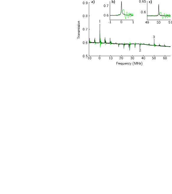
Figure 7: (Color online) a) The hole spectrum of the locking crystal, shown in black, observed after deconvolving the raw transmission, show in green. The peak labeled “1” and shown in inset b) at zero frequency corresponds to the carrier beam. This beam gives rise to several holes and anti-holes in a frequency range of $\pm 36.9$ MHz; the outermost one is labeled “2”. This illustrates that a modulation frequency of $\omega_{\mathrm{m}}=2\pi\cdot 50$ MHz is desirable in order that the side hole, labeled “3” and shown in inset c), does not interfere with the hole spectrum of the carrier beam. The measured line-widths of the peaks shown in insets b) and c) are 60 kHz and 36 kHz for the carrier and sideband holes, respectively. The raw spectrum spanning $-10$ MHz to 70 MHz was collected in 800 µs.

IV.1.2 Phase stability measurement setup

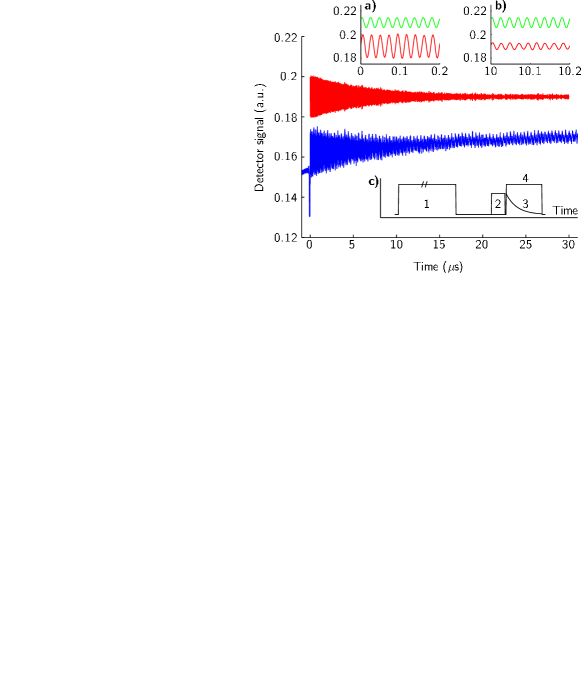
Figure 8: (Color online) Illustration of the phase stability measurements. In the main figure the lower (blue) trace shows the raw detector signal from the heterodyne FID detection. The upper trace (red) shows a filtered version of the lower trace. The lower traces (red) in insets a) and b) show this filtered signal in a 200 ns window around time 0 and 10 µs, respectively. This can be compared to the local oscillator shown by the upper traces (green). We were able to obtain a good SNR for the phase difference of these signals. Inset c) shows the pulse sequence for the experiment: (1) is a 10 ms burn pulse scanning between 40 MHz and 50 MHz (relative to the AOM double-pass center). After waiting 100 µs, pulse (2) with a constant frequency of zero and duration 40 µs sets up a coherence in the atoms which leads to the FID at (3). Finally, pulse (4) at a frequency of 45 MHz beats with the FID signal, leading to the detector signal shown in the main figure (lower, blue trace).

In order to measure the laser stability on short timescales we modified the setup shown in Fig. 6 slightly such that the zeroth-order diffracted beam from AOM 2 (which is not used) is sent to the locking crystal with a beam diameter of roughly 2 mm. AOM 1 is operated around its 200 MHz center frequency and hence, with the frequency shifted around 400 MHz in double pass configuration, the probing beam will not interfere with the laser locking system.

We used optical FID to measure the laser stability and to this end we programmed the pulse sequence shown in Fig. 8(c) and discussed in the figure caption. Referring to this figure, when pulse “2” is applied a coherence is set up in the atomic medium and when pulse “2” is turned off the atoms will keep radiating for a time limited by the optical coherence time, $T_{2}$, (which in our case is around 18 µs) and also by the inverse bandwidth of the actual coherence. This decaying radiation “3” gives a fingerprint of the phase of the laser during pulse “2”. At the same time, we apply another pulse, “4”, shifted 45 MHz in frequency carrying its own phase. The beating of pulses “3” and “4” hence compares the present phase and the past phase, and this allows us to calculate the characteristics of the laser, as discussed in detail in Sec. IV.3.

Fig. 8 illustrates a simple and useful method Takeda1982 of obtaining the amplitude and phase of an oscillating signal, in our case the FID heterodyne signal. The raw detector signal is Fourier transformed and filtered in a 40 MHz bandwidth around the positive 45 MHz component. The fact that the negative frequency components are removed leads (after a subsequent inverse Fourier transform) to a complex representation of the filtered FID signal in the time domain. The phase and amplitude can be read out directly from this complex signal. As an illustration, we show the filtered version of the FID signal in Fig. 8(a,b) together with a 45 MHz local oscillator signal derived from the 1 GHz arbitrary waveform generator. We see that the signals remain in phase over a period of 10 µs. This kind of measurement is repeated 100 times, which allows us to calculate the statistics of the laser stability in a quantitative manner.

IV.2 Long-term drift

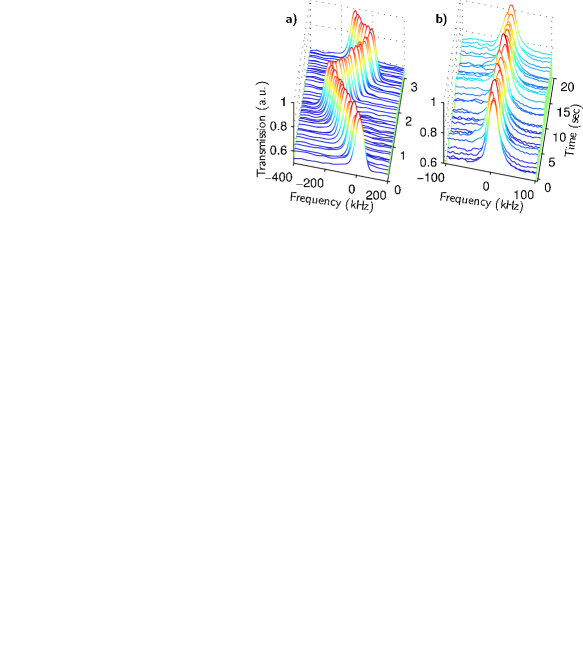
Figure 9: (Color online) Example of drift measurements. a) Total read-out time is 3 seconds and we see a drift rate of roughly 160 kHz/s, while the direction changes occasionally. b) Total read out time is 20 s and the drift is 0.3 kHz/s over this time.

Let us now turn to the experimental results concerning the laser drift and the hole shapes in the locking crystal. In Sec. II.5 we argued that if the spectral holes used for locking are too deep, the laser may be locked but drifting linearly in frequency, which in turn will cause the hole shape to be asymmetric. This is illustrated in Fig. 10(a,b).

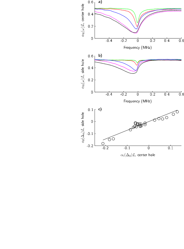
Figure 10: (Color online) In the two upper graphs the measured absorption, $\alpha_{\mathrm{R}}(\omega)L$, is plotted for comparison under different conditions for a number of center holes (a) and side holes (b). With increasing hole depth, the asymmetry of both increases. The imaginary part, $\alpha_{\mathrm{I}}(\Delta_{0})$, of the absorption length at the hole center is a quantitative measure of this asymmetry, and can be calculated from $\alpha_{\mathrm{R}}(\omega)$ using the Kramers-Krönig relations (61). In (c) we see, for several measurements under different conditions, a clear linear relationship between this asymmetry for the center and side holes. The straight line is a fit through the origin with a slope of 0.72, theoretically we expect a slope of unity.

From these measured center and side hole shapes, $\alpha_{\mathrm{R}}(\omega)L$, we can calculate the imaginary parts, $\alpha_{\mathrm{I}}(\omega)L$, by using the Kramers-Krönig relations Jackson1998 . In our case, these relations take a slightly simpler form than usual since in Eq. (4) the only $\omega$-dependence is in the denominator $\frac{\Gamma_{\mathrm{h}}}{2}+i(\Delta-\omega)$. It can be shown that:

$$\begin{split}\alpha_{\mathrm{R}}(\omega_{0})&=+\underset{\delta\rightarrow 0}{\lim}\frac{1}{\pi}\int_{-\infty}^{\infty}\frac{\alpha_{\mathrm{I}}(\omega)(\omega-\omega_{0})d\omega}{(\omega-\omega_{0})^{2}+\delta^{2}},\\ \alpha_{\mathrm{I}}(\omega_{0})&=-\underset{\delta\rightarrow 0}{\lim}\frac{1}{\pi}\int_{-\infty}^{\infty}\frac{\alpha_{\mathrm{R}}(\omega)(\omega-\omega_{0})d\omega}{(\omega-\omega_{0})^{2}+\delta^{2}}.\end{split}$$ (61)

Since $\alpha_{\mathrm{I}}(\omega_{0})$ is an integral of $\alpha_{\mathrm{R}}(\omega)$ times an odd function in $\omega-\omega_{0}$, the value of $\alpha_{\mathrm{I}}(\Delta_{0})$ may be regarded as a convenient measure of the hole asymmetry, which allows us to quantitatively compare the center and side hole shapes. This is shown in Fig. 10(c) for a number of different settings of $T_{\mathrm{10MHz}}$ and $T_{\mathrm{17MHz}}$. We see a clear proportionality, $\alpha_{\mathrm{I}}^{(\mathrm{side})}(\Delta_{0})=0.72\cdot\alpha_{\mathrm{I}}^{(\mathrm{carrier})}(\Delta_{0})$.

We expect $\alpha_{\mathrm{I}}^{(\mathrm{carrier})}(\Delta_{0})$ and $\alpha_{\mathrm{I}}^{(\mathrm{side})}(\Delta_{0})$ to be equal, since from Eq. (6) the phase shifts, of the carrier $\phi_{\mathrm{c}}$ and sideband $\phi_{\mathrm{s}}$ are proportional to $\alpha_{\mathrm{I}}^{(\mathrm{carrier})}(\Delta_{0})$ and $\alpha_{\mathrm{I}}^{(\mathrm{side})}(\Delta_{0})$, respectively, and with a closed laser stabilization feedback loop we must have zero error signal with $\phi_{\mathrm{c}}=\phi_{\mathrm{s}}$. The reason for the slope not being unity is unknown. We have thus shown that the laser may drift linearly, while the feedback loop is still locked. We base this on the direct observations of the drift, as exemplified in Fig. 9(a), on the proportionality in Fig. 10(c), and on the fact that the electronic error signal is small.

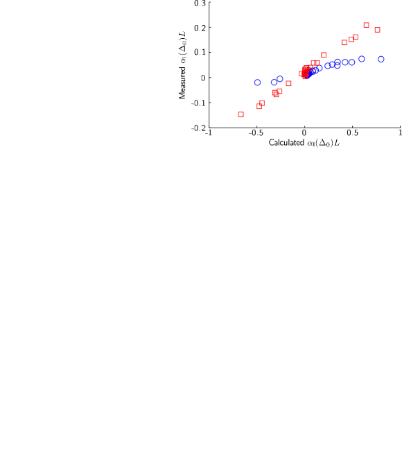
Figure 11: (Color online) Comparison of the measured and calculated imaginary center hole absorption depth, $\alpha_{\mathrm{I}}(\Delta_{0})L$, for different settings of the RF pumping times $T_{\mathrm{17MHz}}=10\cdot T_{\mathrm{10MHz}}$. On the $y$-axis $\alpha_{\mathrm{I}}(\Delta_{0})L$, as inferred from the measured $\alpha_{\mathrm{R}}(\omega)$ via the Kramers-Krönig relations in Eq. (61) is plotted. On the $x$-axis $\alpha_{\mathrm{I}}(\Delta_{0})$ calculated from Eq. (57) with the experimentally inferred values of $\alpha_{0}L$, $\Gamma_{\mathrm{hole,c}}$, $d_{\mathrm{hole,c}}$, $T_{\mathrm{rg}}=T_{\mathrm{gr}}=T_{\mathrm{10MHz}}$, and $\beta$, while $T_{1}=150$ µs and $b_{\mathrm{er}}=0.5$ is plotted. The blue circles and red squares correspond to the data shown in Fig. 12(a) and Fig. 12(c), respectively. These two cases differ by 1 GHz in the position on the inhomogeneous profile, giving background absorptions, $\alpha_{0}L$, of 0.44 and 0.66 for the blue circles and red squares, respectively.

We may also wish to correlate the measured hole asymmetry, $\alpha_{\mathrm{I}}(\Delta_{0})$, with measured drift rate, $\beta$, since these should be related by Eq. (57), at least for small drift rates when the first-order theory is valid. This equation assumes a three-level model, and for our real Pr³⁺:Y₂SiO${}_{5}\,$ions we observe that the $\pm\frac{1}{2},\pm\frac{3}{2}\rightarrow\pm\frac{1}{2},\pm\frac{3}{2}$ transitions with typical branching ratios around 0.5 and hole lifetimes, given mostly by $T_{\mathrm{10MHz}}$, are reasonably representative. Hence, we use $T_{\mathrm{rg}}=T_{\mathrm{gr}}=T_{\mathrm{10MHz}}$ and $b_{\mathrm{er}}=0.5$. Also, from the experimentally measured hole shape parameters, $\Gamma_{\mathrm{hole}}^{(\mathrm{meas})}$ and $d_{\mathrm{hole}}^{(\mathrm{meas})}$, we can estimate $\Gamma_{\mathrm{hole}}$ and $d_{\mathrm{hole}}$ from Eq. (22). Inserting these parameters together with the experimentally determined drift rate, $\beta$, into Eq. (57) we can calculate, to first order, the value of $\alpha_{\mathrm{I}}(\Delta_{0})$ for the center hole. This is plotted on the abscissa in Fig. 11. On the ordinate $\alpha_{\mathrm{I}}(\Delta_{0})$ is plotted, inferred by the Kramers-Krönig relations in Eq. (61) from the measured $\alpha_{\mathrm{R}}(\omega)$. The result shows a proportionality between these two and hence we have demonstrated a clear correlation between measured hole shape asymmetry and measured drift rate as suggested by Eq. (57). The fact that the constant of proportionality is not unity is not alarming since we used a simplified model with only three atomic levels. Also, when the laser is drifting the first-order theory should not be sufficient. The figure shows results from two different experimental runs at two different positions on the inhomogeneous profile. These have a different slope, which is not understood. From the results in Fig. 11 we have demonstrated that the predictions of Eq. (57) show the correct order of magnitude when compared to experiment. It should be borne in mind that a full understanding of the data requires more than our first-order calculations.

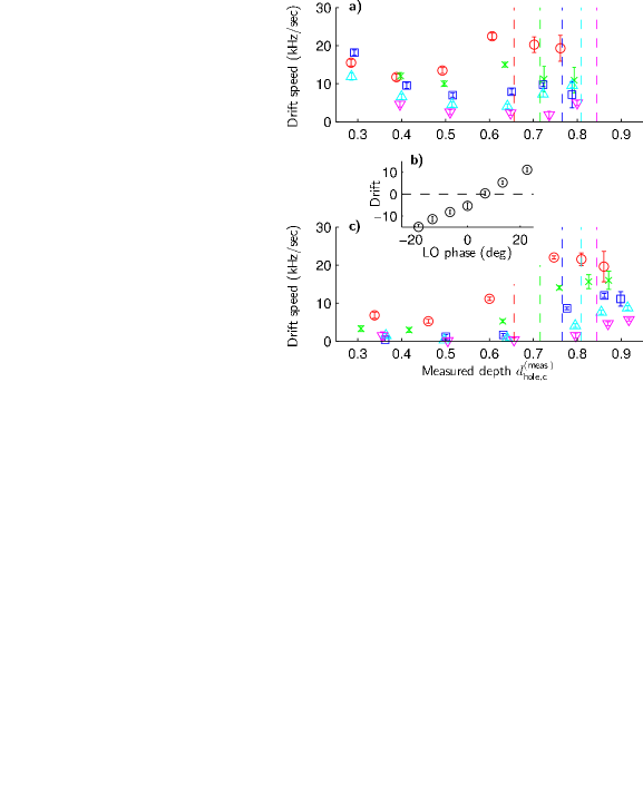
Figure 12: (Color online) Measured drift rates versus measured hole depth. The hole shapes are changed by varying $T_{\mathrm{10MHz}}$ and $T_{\mathrm{17MHz}}$. Red circles, $m=0.56$; green crosses, $m=0.40$; blue squares, $m=0.28$; cyan triangles up, $m=0.20$, purple triangles down, $m=0.14$. The vertical dashed lines indicate the values of the corresponding thresholds shown in Fig. 3. The two graphs differ in that the data shown in (a) were collected before (c) and between the measurements the laser frequency was moved 1 GHz on the inhomogeneous profile, changing the background absorption, $\alpha_{0}L$, from 0.44 to 0.66. In addition, as shown in inset (b), the local oscillator phase (relative to the value used in (a)) to demodulate the error signal, was adjusted in order to minimize the drift rate for shallow holes.

Let us now turn to the measured drift rate, $\beta$, for various parameter settings. The results of these measurements are shown in Fig. 12. The light intensity is kept constant with the saturation parameter $s_{0}\approx 0.09$. The modulation index, $m$, has the values 0.14, 0.20, 0.28, 0.40, and 0.56, and each color in the figure corresponds to one of these values. The hole shapes are controlled by employing $T_{\mathrm{10MHz}}=\frac{1}{10}\cdot T_{\mathrm{17MHz}}$ at the six values 2 ms, 4 ms, 8 ms, 20 ms, 40 ms, and 80 ms. In the figure the six corresponding data points are plotted for each color from left to right since the hole depth $d_{\mathrm{hole,c}}^{(\mathrm{meas})}$ increases with $T_{\mathrm{10MHz}}$.

The results in Fig. 12 are divided into two parts. In Fig. 12(a) we see that the drift rate is lowest for hole depths around 0.5, corresponding to $T_{\mathrm{10MHz}}=8$ ms. For shorter timescales (towards the left) the drift rate tends to increase and this could be caused, for example, by offset errors in the electronics, or by the small signal from the inhomogeneous background if the phase of the local oscillator is set incorrectly. Note, that if the error signal has an offset of $10^{-3}$ times the full-scale value, we would expect the laser to be displaced by $10^{-3}\Gamma_{\mathrm{hole}}$ in frequency. With a hole lifetime of $T_{\mathrm{rg}}$ we can then estimate the drift as $\beta\approx 10^{-3}\Gamma_{\mathrm{hole}}/T_{\mathrm{rg}}$. For our shortest timescales $T_{\mathrm{rg}}\approx 2$ ms, we have $\Gamma_{\mathrm{hole}}/2\pi\approx 40$ kHz leading to an estimate of $\beta/2\pi\approx 20$ kHz/s. This is not far from the experimental values, which we find to be typically a little less than 20 kHz/s and we thus concluded that our relative offset errors are smaller than $10^{-3}$ for the data shown in Fig. 12(a). For longer timescales (towards the right) we can also see an increase in drift rate, which can be explained by the fact that we are approaching the maximum hole depth, discussed around Eq. (59) and Fig. 3. For each color in Fig. 12 this threshold is shown as a vertical dashed line.

The above conclusions become more apparent when we consider Fig. 12(c). Before collecting these data we noted that the drift rate for a shallow hole depends on the position on the inhomogeneous profile, which was then adjusted by 1 GHz. In addition, as shown in the figure inset (b), adjusting the local oscillator phase slightly also has an impact on the drift rate, which we fine tuned to a low value. Fig. 12(c) shows low drift rates in the left part of the figure (the lowest measured being below 0.5 kHz/s). However, the higher drift rates in the right-hand part of the figure remain almost unchanged. A slight change in error signal offset cannot change the fact that zero drift is an unstable solution if the criterion in Eq. (59) is not met. The increase in drift rate on the right-hand side of Fig. 12(c) is now consistent with the vertical lines representing the threshold. The highest drift rate is still below 25 kHz/s which is fairly good.

A very rough order of magnitude estimate of the drift rate can be obtained by noting the fact that the calculations in Sec. II.5 rely on the series expansion in the dimensionless parameter, $\xi=\frac{\beta T_{\mathrm{rg}}}{\Gamma_{\mathrm{hole}}}$. To calculate the threshold condition for $\beta=0$ being a stable solution it is sufficient to assume that $\xi\ll 1$. However, to calculate the actual drift rate when $\beta=0$ is unstable requires higher order theory, where $\xi$ cannot be small. Thus, if we then take for our right-most data points the typical values $T_{\mathrm{rg}}=80$ ms, $\Gamma_{\mathrm{hole}}/2\pi\approx 100$ kHz, and $\beta/2\pi=25$ kHz/s, we obtain $\xi\approx 0.02$, which is actually quite low compared to unity. This is an indication that the fraction of ions resonant on the $\pm\frac{5}{2}\rightarrow\pm\frac{5}{2}$ transition with ten-fold longer hole lifetime, $T_{\mathrm{rg}}=T_{\mathrm{17MHz}}$, and ten-fold higher $\xi$ plays a role in limiting the measured drift rate to a low value. Without having completely searched the very large multi-dimensional parameter space, our experience tells us that $T_{\mathrm{10MHz}}=\frac{1}{10}\cdot T_{\mathrm{17MHz}}$ is a good choice. We have observed examples of much higher drift rates than 25 kHz/s, see e.g. Fig. 9(a) where, in addition to a high drift rate of 160 kHz/s, we also saw that the direction changed occasionally.

IV.3 Short-term phase stability

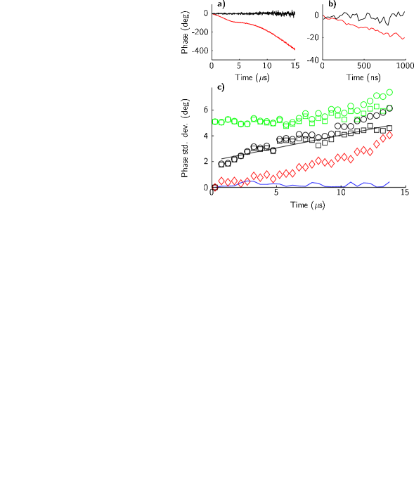
Figure 13: (Color online) (a) A typical single-shot example of the measured FID phase with our stabilization system on (black) and off (red). (b) An enlargement of the first $\mathrm{\SIUnitSymbolMicro}$s of the plot shown in (a). (c) Phase standard deviation versus time, collected in time bins of 500 ns. Red diamonds represent the experimental uncertainty in the measurements, given by Eq. (62). Green circles show the shot-to-shot variations, $\mathrm{std}(x_{i})$. The black circles describe the variation of the phase with respect to the phase of the first time bin, $\mathrm{std}(x_{i}-x_{1})$. The green and black squares show the results when the measurement noise has been subtracted. The blue line shows the absolute value of the mean phase compared to the first time bin. The black line is a linear fit to the black squares, giving $\delta\phi[\mathrm{deg}]=2.0+2.0\cdot 10^{5}t[\mathrm{s}]$.

Fig. 13(a,b) shows the phase evolution of the filtered FID signal for the case when the laser stabilization system is on (black) and off (red). In the latter case, the dye laser is stabilized to a reference cavity by its commercial feedback system. The clear effect of our locking system can be seen, and below we analyze this phase evolution quantitatively.

We note from Fig. 8 that our method based on detection of the FID signal works in practice for times up to around 15 µs. The SNR when determining the phase will decrease with increasing time. Also, referring to Fig. 8(c), the variation in the phase of the laser is present in both the FID signal “3” and in the heterodyning pulse “4”. In order to derive the actual phase stability of the laser we repeated the measurements shown in black in Fig. 13(a) 100 times, divided the measured phase into time bins of length 500 ns, and performed statistical operations on these measured phases. Note, that when discussing the phase of the FID signal we always mean the phase difference between the reference signal and the FID signal (shown in green and red in Fig. 8(a,b), respectively).

In the following, $x_{i,j}$ denotes the measured phase in time bin $i$ for repetition $j=1,\ldots,100$. For each time bin $i$ we may calculate the mean value $\mathrm{bar}{x}_{i}=\frac{1}{n}\sum_{j}x_{i,j}$ and variance $\mathrm{Var}(x_{i})=\frac{1}{n-1}\sum_{j}(x_{i,j}-\mathrm{bar}{x}_{i})^{2}$, where $n=100$. In Fig. 13(c) $\mathrm{abs}(\mathrm{bar}{x}_{i})$ is shown by the blue line and $\mathrm{std}(x_{i})=\sqrt{\mathrm{Var}(x_{i})}$ by the green circles. We see that the average phase deviates less than 1 degree over time, which simply means that there is no phase drift in one particular direction. The $\mathrm{std}(x_{i})$ values describe the repeatability of the experiment, which is within roughly 5 degrees and increases with time. To characterize the measurement noise we now assume a model where the measured values can be written $x_{i,j}=\phi_{i,j}+n_{i,j}$, where $\phi_{i,j}$ is the actual phase of the FID signal and $n_{i,j}$ is a stochastic variable describing the noise in the $i$’th time bin and $j$’th measurement. Since technical laser noise in general is very limited at the heterodyne beating frequency 45 MHz, we assume the noise level to be shot noise or electronic noise in the detector. This is broadband (white) noise and we may assume all the individual $n_{i,j}$ are independent. The mean value is assumed to be equal to zero, and the standard deviation $\mathrm{std}(n_{i})$ will depend on $i$ due to the decaying FID signal. In order to estimate the standard deviation of $n_{i,j}$ we calculate the variance of adjacent time bins for our experimental data:

$$\begin{split}\mathrm{Var}(x_{i}-x_{i-1})&=\mathrm{Var}(\phi_{i}-\phi_{i-1})+\mathrm{Var}(n_{i}-n_{i-1})\\ &\approx\mathrm{const}+2\cdot\mathrm{Var}(n_{i}).\end{split}$$ (62)

In the second step we use the fact that $\mathrm{Var}(\phi_{i}-\phi_{i-1})$ must be time independent since the laser phase is in a steady-state condition. We also use the approximation $\mathrm{Var}(n_{i}-n_{i-1})=\mathrm{Var}(n_{i})+\mathrm{Var}(n_{i+1})\approx 2\mathrm{Var}(n_{i})$, since we assume the detection noise to vary slowly over time. Plotting the variance $\mathrm{Var}(x_{i}-x_{i-1})$ versus time (i.e. plotting Eq. (62) as a function of $i$) will give the measurement noise, $\mathrm{Var}(n_{i})$, and the constant, $\mathrm{Var}(\phi_{i}-\phi_{i-1})$. In Fig. 13(c) $\mathrm{std}(n_{i})=\sqrt{\mathrm{Var}(n_{i})}$ is shown by red diamonds, and is seen to increase from zero to less than 4 degrees at long times.

This noise level can now be used to correct the shot-to-shot variance, shown by the green circles, since $\mathrm{Var}(x_{i})=\mathrm{Var}(\phi_{i})+\mathrm{Var}(n_{i})$. Subtracting the measurement noise, the green squares show the standard deviation, $\mathrm{std}(\phi_{i})$, of the FID signal itself.

When characterizing laser performance it is more interesting to measure the phase evolution over time, i.e. how much the phase of the $i$’th time bin, $\phi_{i}$, deviates from the first one, $\phi_{1}$. To this end we first calculate $\mathrm{Var}(x_{i}-x_{1})=\mathrm{Var}(\phi_{i}-\phi_{1})+\mathrm{Var}(n_{i}-n_{1})$ from the experimental data. The square root of this is $\mathrm{std}(x_{i}-x_{1})$, which is plotted in Fig. 13(c) as black circles. Since $\mathrm{Var}(n_{i}-n_{1})=\mathrm{Var}(n_{i})+\mathrm{Var}(n_{1})=\mathrm{Var}(n_{i})$, we can subtract the measurement noise again to obtain $\mathrm{std}(\phi_{i}-\phi_{1})$, which is plotted as black squares. We see that on short timescales the phase error is around 2 degrees, and it increases linearly with time. The black line in the figure is a linear fit to the black squares, and it can be used to convert the phase stability into a characteristic frequency stability as a function of time. Since the relation between phase and frequency is $\phi[\mathrm{deg}]=360\cdot f[\mathrm{Hz}]\cdot t+\phi_{0}$, the standard deviations of these will be connected by:

$$\mathrm{std}(f)=\frac{\mathrm{std}(\phi)}{360\cdot t}=\frac{2.0+2.0\cdot 10^{5}t}{360\cdot t}$$ (63)

In the second step, we inserted the experimental linear fit shown as the black line in Fig. 13(c). For large $t$ the characteristic frequency standard deviation, $\mathrm{std}(f)$, approaches 0.6 kHz, but we are not allowed to extend $t$ further than the measured 14 µs. Note, for $t=10$ µs, $\mathrm{std}(f)=1.1$ kHz.

The difference between the shot-to-shot standard deviation, plotted in green in Fig. 13(c), and the time separation standard deviation, shown in black in Fig. 13(c), is approximately 3 degrees. The extra noise in the shot-to-shot data arises from the fact that the laser phase also fluctuates during the setup of the coherence in the atoms (pulse “2” in Fig. 8). The practical phase memory time is approximately 10 µs, corresponding to the decay time of the FID signal in Fig. 8. Averaged over 10 µs, the black data points of Fig. 13 actually suggest approximately 3 degrees fluctuation in the laser phase. Thus the data shown in green and black in Fig. 13 are consistent with each other.

The experimental data shown in Fig. 13(c) were obtained with $T_{\mathrm{10MHz}}=\frac{1}{10}\cdot T_{\mathrm{17MHz}}=4$ ms, modulation index $m=0.20$, and saturation parameter $s_{0}\approx 0.09$. This setting is also represented in Fig. 12(c) giving a drift of $(0.34\pm 0.76)$ kHz/s. Hence, we have shown that a slow drift and low phase variations can be obtained at the same time. Of the settings investigated the best general phase stability performance is found for the above RF-eraser time, which gives rise to a measured hole depth, $d_{\mathrm{hole,c}}^{(\mathrm{meas})}$, around 0.5 to 0.6 in Fig. 12. This hole depth corresponds to $x=\frac{\Gamma_{\mathrm{hole}}}{\Gamma_{\mathrm{h}}}\approx 2$, which is the best choice according to the $f$-function (38) shown in Fig. 1. At other settings we still find asymptotic values of Eq. (63) less than 2.5 kHz, which is only four times worse than the value of 0.6 kHz in the example above.

We have also investigated a few different positions on the inhomogeneous profile. These measurements indicate that a transmission above 30% is a good choice. Varying in the local oscillator phase between the values shown in Fig. 12(b) does not change the performance on short timescales.

The performance of the non-stabilized laser, i.e. when the dye laser is operated only with its built-in stabilization unit, is exemplified in Fig. 13(a,b). We see that in this case it takes roughly 13 µs to change the phase by $360^{\circ}$, which can be translated into a characteristic frequency of 75 kHz. Repeating this measurement 100 times shows that these values are typical. In our experience, cooling the laser dye affects this frequency considerably (we typically use temperatures in the range 8  to 12).

The above observation does not mean that the unstabilized laser line-width is 75 kHz, it only means that on short timescales of the order of 10 µs, the frequency deviations are around 75 kHz. In Zhu1993 a typical dye laser line-width of 450 kHz is reported, but it was also indicated that the frequency deviations had a bandwidth $B\ll 190$ kHz, i.e. the deviations occurred on a timescale much longer than 5 µs. Our observations are consistent with this behavior.

As discussed in Sec. III, the group delay of our stabilization feedback loop is approximately 100 ns. To understand how this limits the phase stability of our laser we assumed that the dye laser introduces a frequency error of 75 kHz. It takes 100 ns for the stabilization loop to discover this and start counteracting it, and after this time the phase has evolved roughly $360^{\circ}\cdot 75\>\mathrm{kHz}\cdot 100\>\mathrm{ns}=2.7^{\circ}$. This hand-waving argument is consistent with a standard deviation of the order of 2 degrees, as shown by the data (black squares) in Fig. 13(c) as the limiting case for short timescales. Another way of saying this is that in Fig. 13(b) the typical stabilized phase deviation (shown in black) corresponds to the actual deviation of the non-stabilized laser (shown in red) after a time of the order of the delay time in the feedback loop.

IV.4 Overall laser performance

In summary, we can say that we achieved 1 kHz line-widths on the timescale of 10 µs, and drift stabilities also around 1 kHz on 1 s timescales. We were not able to thoroughly examine the stability on intermediate timescales. If we had had two identical lasers with which to calculate the Allen deviation from beating experiments, our reported line widths should be multiplied by $\sqrt{2}$ for short timescales (with random shifts) and by 2 for long timescales (with linear drift). Then we can compare our laser performance with others reported in the literature.

Laser stabilization using a spectral hole has been reported for semiconductor lasers in several publications Pryde2001 ; Pryde2002 ; Strickland2000 ; Sellin2001 ; Bottger2001 ; Sellin1999 ; Bottger2003 . In these cases the reported Allen deviation on a 10 µs timescale is typically 10 kHz, and around 3 kHz in Strickland2000 . For long timescales a linear drift rate of 10 kHz/s has been observed in pure transient systems Strickland2000 . Stabilities better than our reported 1 kHz/s can be obtained with permanent spectral holes (25 kHz/min) Sellin1999 , ($\approx 1$ kHz/min) Bottger2003 or by incorporating the permanent reference consisting of the inhomogeneous profile (7 kHz/min) Strickland2000 , (1.4 kHz/min, no hole burning) Bottger2007 .

The most important steps in obtaining our short-term phase stability of down to 2 degrees, consist of (1) constructing fast analog electronics to obtain short delays and low noise, (2) using a large sample crystal diameter (19 mm) in order to be able to use a high light power without too high an intensity, and (3) cooling the laser dye in order to improve the passive stability. We should also mention that the optical table is placed on legs with pneumatic vibration dampers, that an improved dye jet nozzle (Radiant Dyes RDSN 02) and an improved nozzle holder and pump mirror adjustment unit (Radiant Dyes RDU 10) have been installed, and that the entire laser system is located inside a clean room (from Terra Universal). In order to obtain the low frequency drift of 1 kHz/s the important steps are: (1) being aware of the drift problem discussed in Secs. II.5 and IV.2 and (2) carefully constructing the electronics so as to ensure low offsets.

IV.4.1 Impacts on quantum gate experiments

As we discussed in the introduction in Sec. I, our main reason for frequency stabilizing the laser is to enable quantum computation experiments. One experimental approach utilizes spectral hole burning to isolate strongly interacting qubits, as described in Nilsson2004 ; Rippe2005 . Such qubit structures will typically have a spectral width of $\approx 200$ kHz, and can be prepared by several hundred cycles of optical pumping. The entire preparation process may take hundreds of milliseconds, and it is important that the laser drift is much less than 200 kHz during this time. With typical drift rates of 1 kHz/s we have fulfilled this requirement.

Let us now consider the effects of laser phase fluctuations on the fidelity of qubit operations. We use two ground state hyperfine levels to represent a qubit, e.g. $\left|0\right>=\left|\pm\frac{1}{2}\right>$ and $\left|1\right>=\left|\pm\frac{3}{2}\right>$. Single qubit operations can be performed by interaction with an excited state $\left|e\right>$ Roos2004 where $\pi$-pulses are used to transfer the population from $\left|0\right>$ or $\left|1\right>$ to $\left|e\right>$ and back again. Such basic operations are also building blocks for more complicated gates, e.g. the CNOT gate Ohlsson2002 ; Roos2004 . Here we will estimate the impact of a phase error in the laser on such a simple operation.

Consider the following scenario. The qubit is in an initial state $\left|\psi_{0}\right>=\alpha\left|0\right>+\beta\left|1\right>$, then a perfect laser drives a $\pi$-pulse on the $\left|1\right>\rightarrow\left|e\right>$ transition such that $\left|\psi_{0}\right>\rightarrow\alpha\left|0\right>+\beta\left|e\right>$. The laser phase is now assumed to change by an amount $\phi$, and we finally drive the excited state back to the final state $\psi_{\mathrm{f}}=\alpha\left|0\right>+\beta e^{i\phi}\left|1\right>$. We have thus gathered all the phase fluctuations in a single step. If there is no phase change ($\phi=0$) we arrive back at the initial state $\left|\psi_{0}\right>$, and the deviation from this can be used to estimate the fidelity of the operation given $\phi$.

However, with an unknown random phase change, $\phi$, the correct description of the final state is given by the density matrix:

$$\begin{split}\hat{\rho}_{\mathrm{f}}&=\int\left|\psi_{\mathrm{f}}\right>\negthickspace\left<\psi_{\mathrm{f}}\right|f(\phi)d\phi=|\alpha|^{2}\left|0\right>\negthickspace\left<0\right|+|\beta|^{2}\left|1\right>\negthickspace\left<1\right|\\ &\quad+\int\left(\alpha\beta^{*}e^{-i\phi}\left|0\right>\negthickspace\left<1\right|+\alpha^{*}\beta e^{i\phi}\left|1\right>\negthickspace\left<0\right|\right)f(\phi)d\phi,\end{split}$$ (64)

where $f(\phi)$ is the probability distribution of the phase change, $\phi$, where $\int f(\phi)d\phi=1$. Given an initial state $\left|\phi_{0}\right>$ the fidelity of the operation is the overlap:

$$\begin{split}F&=\left<\psi_{0}\right|\hat{\rho}_{\mathrm{f}}\left|\phi_{0}\right>=|\alpha|^{4}+|\beta|^{4}+2|\alpha|^{2}|\beta|^{2}\negthickspace\int\negthickspace f(\phi)\cos\phi d\phi\\ &=1-2|\alpha|^{2}|\beta|^{2}\epsilon\qquad\text{with }\epsilon=1-\int\negthickspace f(\phi)\cos\phi d\phi.\end{split}$$ (65)

The parameter $\epsilon$ is zero when there is no phase change ($f(\phi)=\delta(\phi)$) and varies to second order in the phase deviation. To see this clearly we assume a simple top-hat distribution function, $f(\phi)=\frac{1}{2\sqrt{3}\phi_{0}}$ if $-\sqrt{3}\phi_{0}<\phi<\sqrt{3}\phi_{0}$ and zero elsewhere. This distribution function corresponds to a root mean square phase $\phi_{0}$. Inserting this in Eq. (65) gives $\epsilon=\frac{1}{2}\phi_{0}^{2}$ and $F=1-|\alpha|^{2}|\beta|^{2}\phi_{0}^{2}$ when $\phi_{0}\ll 1$.

The phase fluctuation plays no role if the initial state is either of the basis states, $\left|0\right>$ or $\left|1\right>$. The impact is maximal if the initial state is an even superposition with $|\alpha|^{2}=|\beta|^{2}=\frac{1}{2}$. In the latter case, for a phase error with a standard deviation as high as 10 degrees, the fidelity is 98.5%.

More detailed analysis is naturally required to accurately calculate the fidelity loss of entire quantum gate experiments given our laser stability, which is outside the scope of this paper. However, with the above investigations, we are confident that the laser stability is sufficient for our intended quantum gate experiments.

V Outlook

As discussed in Sec. IV.4.1, we have a laser in a sufficiently stable condition for quantum information experiments, which was the main reason for the entire stabilization project. Compared to previous laser stabilization studies on pure transient hole-burning systems, we have achieved better stability, and the understanding of laser drift was very important in this process. However, some compromises had to be made since the absence of linear drift does not necessarily coincide with the maximization of error signals. The presence of both the center and side holes is responsible for this effect, and a number of measures can be taken. (1) An interferometric setup can be considered where only the beam not passing the atoms is modulated in the Pound-Drever-Hall scheme. This, however, requires a very stable or an otherwise stabilized interferometer, since the error signal from the spectral hole locking can not conveniently distinguish whether phase changes occur relative to the atoms or because of instabilities in the interferometer. (2) Moving the modulation side bands outside the inhomogeneous profile. This is inconvenient in our case with Pr³⁺:Y₂SiO${}_{5}\,$since the inhomogeneous broadening is around 5 GHz. However, the system under consideration in Bottger2007 is interesting in this respect. Note, that the drift problem decreases when $\omega_{\mathrm{m}}/\Gamma_{\mathrm{inh}}$ approaches unity, so a combination of the inhomogeneous profile for permanent stability together with hole burning effects for short-term stability may be possible without suffering too strong constraints from the drift criterion when $\omega_{\mathrm{m}}\approx\Gamma_{\mathrm{inh}}$.

In any case, our work has also shown that offset levels and systematic effects must be carefully controlled to achieve low drift rates in pure transient systems. For this reason, the incorporation of permanent effects seems to be the most convenient and competitive solution for obtaining a slow long-term drift. It is our hope that the work presented here will help to further improve the already advanced field of laser stabilization.

VI Conclusions

We have for the first time stabilized a dye laser to a spectral hole in Pr³⁺:Y₂SiO${}_{5}\,$, obtaining 1 kHz frequency stability on a 10 µs timescale, and a long-term drift rate below 1 kHz/s. The use of RF fields to control the hyperfine level populations allowed us to optimize the spectral hole parameters for best laser performance. The stabilities obtained were sufficient for high-fidelity quantum information experiments.

We have contributed to the theoretical understanding of laser stabilization using spectral holes to an extent that we hope will enable other scientists to further improve existing technology. Although a few experimental observations reported in this paper are not fully understood in a quantitative manner, we have provided strong experimental support to the theory describing laser drift.

References

- (1) N. Ohlsson, R. K. Mohan, and S. Kröll, Opt. Commun. 201, 71 (2002).
- (2) I. Roos and K. Mølmer, Phys. Rev. A 69, 022321 (2004).
- (3) J. J. Longdell and M. J. Sellars, Phys. Rev. A 69, 032307 (2004).
- (4) J. J. Longdell, M. J. Sellars, and N. B. Manson, Phys. Rev. Lett. 93, 130503 (2004).
- (5) J. H. Wesenberg, K. Mølmer, L. Rippe, and S. Kröll, e-print quant-ph/0601141.
- (6) R. W. Equall, Y. Sun, R. L. Cone, and R. M. Macfarlane, Phys. Rev. Lett. 72, 2179 (1994).
- (7) R. W. Equall, R. L. Cone, and R. M. Macfarlane, Phys. Rev. B 52, 3963 (1995).
- (8) E. Fraval, M. J. Sellars, and J. J. Longdell, Phys. Rev. Lett. 92, 077601 (2004).
- (9) E. Fraval, M. J. Sellars, and J. J. Longdell, Phys. Rev. Lett. 95, 030506 (2005).
- (10) M. Nilsson et al., Phys. Rev. B 70, 214116 (2004).
- (11) L. Rippe et al., Phys. Rev. A 71, 062328 (2005).
- (12) R. W. P. Drever et al., Appl. Phys. B 31, 97 (1983).
- (13) J. Hough et al., Appl. Phys. B 33, 179 (1984).
- (14) J. Helmcke et al., Appl. Phys. B 43, 85 (1987).
- (15) M. Houssin, M. Jardino, B. Gely, and M. Desaintfuscien, Opt. Lett. 13, 823 (1988).
- (16) R. Kallenbach et al., Opt. Commun. 70, 56 (1989).
- (17) I. Steiner et al., Appl. Phys. B 49, 251 (1989).
- (18) M. Zhu and J. L. Hall, in Proceedings of the 1992 IEEE Frequency Control Symposium (Hershey, Pennsylvania, 1992), pp. 44–55.
- (19) M. Zhu and J. L. Hall, J. Opt. Soc. Am. B 10, 802 (1993).
- (20) M. J. Sellars, Ph.D. thesis, Australian National University, 1995.
- (21) B. C. Young, F. C. Cruz, W. M. Itano, and J. C. Bergquist, Phys. Rev. Lett. 82, 3799 (1999).
- (22) P. B. Sellin, N. M. Strickland, J. L. Carlsten, and R. L. Cone, Opt. Lett. 24, 1038 (1999).
- (23) N. M. Strickland et al., Phys. Rev. B 62, 1473 (2000).
- (24) G. J. Pryde, T. Böttger, and R. L. Cone, J. Lumin. 94-95, 587 (2001).
- (25) G. J. Pryde, T. Böttger, R. L. Cone, and R. C. C. Ward, J. Lumin. 98, 309 (2002).
- (26) P. B. Sellin et al., Phys. Rev. B 63, 155111 (2001).
- (27) T. Böttger et al., J. Lumin. 94, 565 (2001).
- (28) T. Böttger, G. J. Pryde, and R. L. Cone, Opt. Lett. 28, 200 (2003).
- (29) K. D. Merkel et al., Opt. Lett. 25, 1627 (2000).
- (30) L. Rippe, Ph.D. thesis, Division of Atomic Physics, LTH, P.O. Box 118, SE 221 00 Lund, 2006.
- (31) Laser stabilization system documentation, available at http://www.atom.fysik.lth.se/QI/.
- (32) E. D. Black, Am. J. Phys. 69, 79 (2001).
- (33) D. Allen and J. H. Eberly, Optical resonace and two-level atoms (Wiley, New York, 1975).
- (34) P. W. Milonni and J. H. Eberly, Lasers (John Wiley & Sons, New York, 1988).
- (35) L. Mandel and E. Wolf, Optical Coherence and Quantum Optics (Cambridge University Press, New York, 1995).
- (36) M. Abramowitz and I. A. Stegun, Handbook of Mathematical Functions (Dover, New York, 1972).
- (37) A. M. Stoneham, Rev. Mod. Phys. 41, 82 (1969).
- (38) J. H. Wesenberg and K. Mølmer, Phys. Rev. Lett. 93, 143903 (2004).
- (39) G. C. Bjorklund, M. D. Levenson, W. Lenth, and C. Ortiz, Appl. Phys. B 32, 145 (1983).
- (40) T. Böttger, G. J. Pryde, C. W. Thiel, and R. L. Cone, in Proceedings on Ninth International Conference on Hole Burning, Single Molecule and Related Spectroscopies (HBSM 2006), to appear in J. Lumin.
- (41) C. Salomon, D. Hils, and J. L. Hall, J. Opt. Soc. Am. B 5, 1576 (1988).
- (42) N. Hamilton, Radio Communications, p. 39, April 1991.
- (43) K. J. Åström and R. J. Murray, Feedback Systems: An Introduction for Scientists and Engineers, preprint at http://www.cds.caltech.edu/~murray/amwiki/.
- (44) P. C. D. Hobbs, Appl. Opt. 36, 903 (1997).
- (45) F. Wolf, J. Phys. D 27, 1774 (1994).
- (46) T. Chang et al., Opt. Lett. 30, 1129 (2005).
- (47) M. Takeda, H. Ina, and S. Kobayashi, J. Opt. Soc. Am. B 72, 156 (1982).
- (48) J. D. Jackson, Classical Electrodynamics (John Wiley & Sons, New York, 1988).