Semiclassical quantization of an $N$-particle Bose-Hubbard model

Abstract

A semiclassical Bohr-Sommerfeld approximation is derived for an $N$-particle, two-mode Bose-Hubbard system modeling a Bose-Einstein condensate in a double-well potential. This semiclassical description is based on the ‘classical’ dynamics of the mean-field Gross-Pitaevskii equation and is expected to be valid for large $N$. We demonstrate the possibility to reconstruct quantum properties of the $N$-particle system from the mean-field dynamics. The resulting semiclassical eigenvalues and eigenstates are found to be in very good agreement with the exact ones, even for small values of $N$, both for subcritical and supercritical particle interaction strength where tunneling has to be taken into account.

I Introduction

Even for weakly interacting particles, a full many-body treatment of Bose-Einstein condensates (BEC) is only possible for a small number $N$ of particles. Most often a mean-field approximation is used, which describes the system quite well for large $N$ at low temperatures. In this mean-field approach, the bosonic field operators are replaced by c-numbers, the condensate wavefunctions. This constitutes a classicalization and therefore the result of the mean-field approximation, the Gross-Pitaevskii equation (GPE), is often denoted as ‘classical’, despite of the fact that the GPE is manifestly quantum, i.e. it reduces to the usual linear Schrödinger equation for vanishing interparticle interaction. Therefore, in order to avoid misunderstanding, this inversion of the second quantization may be called a second classicalization.

In a number of recent papers, consequences of the classical nature of the mean-field approximation are discussed and semiclassical aspects are introduced. For a two-mode Bose-Hubbard model, Anglin and Vardi Vard01b ; Angl01 consider equations of motion which go beyond the standard mean-field theory by including higher terms in the Heisenberg equations of motion. The classical-quantum correspondence has been studied in terms of phase space (Husimi) distributions Mahm05 for such systems. Mossmann and Jung Moss06 demonstrate for a three-mode Bose-Hubbard model that the organization of the $N$-particle eigenstates follows the underlying classical, i.e. mean-field, dynamics. A generalized Landau-Zener formula for the mean-field description of interacting BECs in a two-mode system has been derived by studying the many particle system 06zener_bec . In Wu06 the commutability between the classical and the adiabatic limit for the same system is studied and first steps towards a semiclassical treatment of the problem are reported.

The purpose of the present paper is to show that the mean-field model is not only capable to approximate the interacting $N$-particle system in the limit of large $N$ and to allow for an interpretation of the organization of the $N$-particle eigenvalues and eigenstates, but can also be used to reconstruct approximately the individual eigenvalues and eigenstates in a semiclassical Bohr-Sommerfeld (or EBK) manner with astounding accuracy even for a small number of particles. This will be demonstrated for $N$ bosonic particles in a two-mode system, a many-particle Bose-Hubbard Hamiltonian, describing for example the low-energy dynamics of a BEC in a (possibly asymmetric) double-well potential. This system is related to a classical non-rigid pendulum in the mean-field approximation (see, e.g., Mahm05 and references therein).

Both the many particle model and its classical version – which is often denoted as the discrete self-trapping equation for reasons which will become obvious in the following – have been studied for decades in different context (see semiMP_Bem2 ). A detailed semiclassical analysis is, however, missing up to now. Previous work in this direction concentrated on the symmetric case, where the permutational symmetry of the system with respect to an interchange of the two modes simplifies an analysis. Semiclassical expressions for the tunneling splittings of the eigenvalues have been derived Enz86 ; Scha87 in context of the spin-system in eqn. (2) below (see also Bern90 ; Gara91 for a perturbative treatment of the splittings and Fran01 for a detailed analysis of the quantum spectrum).

In the following we will first give a short overview of the many particle description of the model, the celebrated mean-field approximation and their correspondence. Afterwards we focus on the question to which extent many particle properties can be extracted from the mean-field system by an inversion of this ‘classical’ approximation in a semiclassical way using the EBK-quantization method Brac97 .

II Two-mode Bose-Hubbard model and mean-field approximation

In a two-mode approximation at low temperatures a BEC in a double-well potential can be described by a second quantized many particle Hamiltonian of Bose-Hubbard type:

$$\hat{H}=\varepsilon(\hat{n}_{1}-\hat{n}_{2})+v(\hat{a}_{1}^{\dagger}\hat{a}_{2}+\hat{a}_{2}^{\dagger}\hat{a}_{1})+g\left(\hat{n}_{1}^{2}+\hat{n}_{2}^{2}\right)\,.$$ (1)

Here $\hat{a}_{j}$, $\hat{a}_{j}^{\dagger}$ are bosonic particle annihilation and creation operators for the jth mode and $\hat{n}_{j}=\hat{a}_{j}^{\dagger}\hat{a}_{j}$ are the mode number operators. The mode energies are $\pm\varepsilon$, $v$ is the coupling constant and $g$ is the strength of the onsite interaction. In order to simplify the discussion, we assume here that $v$ is positive and $g$ is negative semiMP_Bem1 . The Hamiltonian (1) commutes with the total number operator $\hat{N}=\hat{n}_{1}+\hat{n}_{2}$ and the number $N$ of particles, the eigenvalue of $\hat{N}$, is conserved. For a given value of $N$, we have $N+1$ eigenvalues of the Hamiltonian (1). Alternatively, the system can be described in the Schwinger representation by transformation to angular momentum operators $\hat{J}_{x}=(\hat{a}_{1}^{\dagger}\hat{a}_{2}+\hat{a}_{2}^{\dagger}\hat{a}_{1})/2$ , $\hat{J}_{y}=(\hat{a}_{1}^{\dagger}\hat{a}_{2}-\hat{a}_{2}^{\dagger}\hat{a}_{1})/2{\rm i}$ , $\hat{J}_{z}=(\hat{a}_{1}^{\dagger}\hat{a}_{1}-\hat{a}_{2}^{\dagger}\hat{a}_{2})/2$ . The Hamiltonian (1) then takes the form

$$\hat{H}=2\varepsilon\hat{J}_{z}+2v\hat{J}_{x}+2g(\hat{J}_{z}^{2}+N^{2}/4),$$ (2)

where the total angular momentum is $J=N/2$.

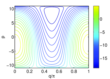
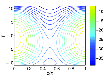
Figure 1: (Color online) Phase space portrait of the mean-field Hamiltonian ${\cal H}(p,q)$ in (5) for $v=1$ and $\varepsilon=-0.5$ in the subcritical ($g=-1/N_{s}$, top) and supercritical ($g=-3/N_{s}$, bottom) region for $N=10$ and $\hbar=1$.

The celebrated mean-field description can be most easily formulated as a replacement of operators by c-numbers $\hat{a}_{j}\rightarrow\psi_{j}$, $\hat{a}_{j}^{\dagger}\rightarrow\psi_{j}^{*}$. Since the c-numbers commute in contrast to the quantum mechanical operators, the transition quantum $\to$ classic and vice versa is not one-to-one. To avoid ambiguities one has to replace symmetrized products of the operators by the corresponding products of c-numbers. Therefore we will start on the many particle side with a symmetrized Bose-Hubbard Hamiltonian in the following, where the $\hat{n}_{j}$ are replaced by $\hat{n}^{s}_{j}=(\hat{a}_{j}^{\dagger}\hat{a}_{j}+\hat{a}_{j}\hat{a}_{j}^{\dagger})/2$ (see also Moss06 ). This symmetrization affects only the nonlinear term in (1) and the symmetrized $\hat{H}$ is related to (1) by an additive constant term depending only on $\hat{N}$. Note that thus the number operator $\hat{N}=\hat{n}_{1}+\hat{n}_{2}=\hat{n}^{s}_{1}+\hat{n}^{s}_{2}-\hat{1}$ is replaced by $|\psi_{1}|^{2}+|\psi_{2}|^{2}-1$ and therefore the mean-field wavefunction is normalized as $|\psi_{1}|^{2}+|\psi_{2}|^{2}=N+1=N_{s}$.

The mean-field time evolution is given by the two level nonlinear Schrödinger equation, resp. GPE,

$${\rm i}\hbar\,\frac{{\rm d}}{{\rm d}t}\begin{pmatrix}\psi_{1}\\ \psi_{2}\end{pmatrix}=\begin{pmatrix}\varepsilon+2g|\psi_{1}|^{2}&v\\ v&-\varepsilon+2g|\psi_{2}|^{2}\end{pmatrix}\begin{pmatrix}\psi_{1}\\ \psi_{2}\end{pmatrix}\,,$$ (3)

where $\psi_{1}$ and $\psi_{2}$ are the amplitudes of the two condensate modes.

The Schrödinger equation, linear or nonlinear, has the canonical structure of classical dynamics Ablo04 ; Fadd87 ; Hesl85 : The time dependence of the complex valued mean-field amplitudes can be written as canonical equations of motion

$${\rm i}\hbar\frac{{\rm d}\psi_{j}}{{\rm d}t}=\frac{\partial{\cal H}}{\partial\psi_{j}^{*}}\quad\text{and}\quad{\rm i}\hbar\frac{{\rm d}\psi_{j}^{*}}{{\rm d}t}=-\frac{\partial{\cal H}}{\partial\psi_{j}}$$ (4)

with a Hamiltonian function ${\cal H}=\epsilon(|\psi_{1}|^{2}-|\psi_{2}|^{2})+v(\psi_{1}^{*}\psi_{2}+\psi_{1}\psi_{2}^{*})+g(|\psi_{1}|^{4}+|\psi_{2}|^{4})$. The conservation of the particle number allows a reduction of the dynamics to an effectively one-dimensional Hamiltonian evolution by an amplitude-phase decomposition $\psi_{j}=\sqrt{n_{j}+1/2}\,{\rm e}^{{\rm i}q_{j}}$ in terms of the canonical coordinate $q=(q_{1}-q_{2})/2$, an angle, and the (angular)momentum $p=(n_{1}-n_{2})\hbar$, with the Hamiltonian function

$${\cal H}(p,q)=\varepsilon\,\frac{p}{\hbar}+v\sqrt{N_{s}^{2}-\frac{p^{2}}{\hbar^{2}}}\,\cos(2q)+\frac{g}{2}\big{(}N_{s}^{2}+\frac{p^{2}}{\hbar^{2}}\big{)}\,,$$ (5)

where $N_{s}$ is the normalization of $\psi$. Introducing the new variables the canonical equations of motion (4) obtain their usual appearance $\dot{q}=\partial{\cal H}/\partial p$ and $\dot{p}=-\partial{\cal H}/\partial q$:

$$\dot{p}= 2v\sqrt{N_{s}^{2}-\frac{p^{2}}{\hbar^{2}}}\sin(2q)$$ (6)

$$\dot{q}= \frac{\varepsilon}{\hbar}-v\frac{p}{\hbar^{2}\sqrt{N_{s}^{2}-\frac{p^{2}}{\hbar^{2}}}}\,\cos(2q)+g\frac{p}{\hbar^{2}}.$$ (7)

This describes the classical dynamics of a non-rigid pendulum where the phase space is finite, $-N_{s}\hbar\leq p\leq N_{s}\hbar$, $0\leq q\leq\pi$, if the lines $q=0$ and $q=\pi$ are identified.

One of the prominent features of the two-mode system is the self-trapping effect, which leads to the emergence of additional stationary states favoring one of the wells above a critical particle interaction strength. For a discussion of the relation between mean-field and $N$-particle behavior see, e.g., Aubr96 ; Milb97 and references therein and Holt01a for its control by external driving fields. The self-trapping transition occurs at $g=-v/N_{s}$ and is connected to a bifurcation of the stationary states, the fixed points of the Hamiltonian (5), in the mean-field approximation. Figure 1 shows phase space portraits of ${\cal H}(p,q)$ for sub- and supercritical particle interaction strength. In the subcritical region one has a maximum, $E^{+}$, at $q=0$ and a minimum, $E^{-}$, at $q=\pi/2$. For the symmetric case $\varepsilon=0$, both are located at $p=0$, which means that the population in both wells is the same. In the supercritical region the minimum bifurcates into two minima, $E^{-}_{\pm}$, and a saddle point, $E^{-}_{\rm saddle}>E^{-}_{\pm}$. Even for the case $\varepsilon=0$ the two minima are located at a finite value of the population imbalance. In these stationary states the condensate mainly populates one of the wells, which leads to the name self-trapping. In phase space, the regions with oscillations around one of the two minima are separated by a separatrix passing through the saddle point. The period of the separatrix motion is infinite.

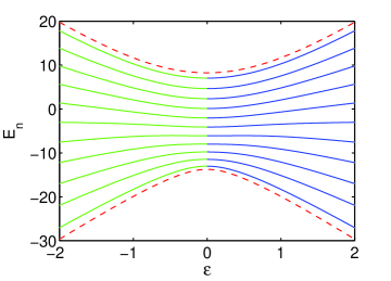
Figure 2: (Color online) Many particle energies $E_{n}$ and mean-field eigenenergies ${\cal H}_{stat}$ (- -) as a function of the onsite energy $\varepsilon$ in the subcritical region ($g=-0.5/N_{s}$) for $v=1$ and $N=10$ particles ($\hbar=1$). The spectrum is organized by the mean-field eigenenergies ${\cal H}_{stat}$ (- -). The exact quantum eigenvalues shown for $\varepsilon\leq 0$ (—) are almost exactly reproduced by the semiclassical ones, $E_{n}^{sc}$, shown for $\varepsilon\geq 0$ (—).

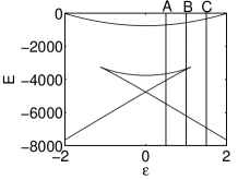
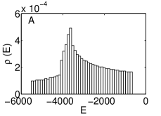
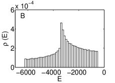
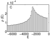
Figure 3: Level density $\varrho(E)$ of the many particle system in comparison to the mean-field energies for $N=1500$ particles for $v=1$, $g=-3/N_{s}$ and $\varepsilon=0.5,1,1.5$ ($\hbar=1$).

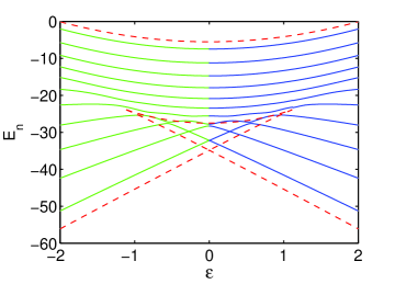
Figure 4: (Color online) Many particle energies $E_{n}$ and mean-field eigenenergies ${\cal H}_{stat}$ (- -) as a function of the onsite energy $\varepsilon$ in the supercritical region ($g=-3/N_{s}$) for $v=1$ and $N=10$ particles ($\hbar=1$). The spectrum is organized by the mean-field eigenenergies ${\cal H}_{stat}$ (- -). The exact quantum eigenvalues shown $\varepsilon\leq 0$ (—) are almost exactly reproduced by the semiclassical ones, $E_{n}^{sc}$, shown for $\varepsilon\geq 0$ (—).

Figure 2 shows an example of the many particle eigenvalues $E_{n}$ in dependence on $\varepsilon$ for a subcritical interaction strength. The pattern of eigenvalues varies smoothly with $\varepsilon$ and is bounded by the stationary mean-field energies shown as red curves. Because of the symmetry of the spectrum for $\varepsilon\rightarrow-\varepsilon$ the exact spectrum is only shown for $\varepsilon\leq 0$, whereas for $\varepsilon\geq 0$ the semiclassical eigenvalues are shown as discussed below. Figure 4 shows a similar plot in the supercritical region. Here we observe a net of avoided crossings clearly organized by a skeleton provided by the stationary mean-field energies, as reported before by several authors Kark02 ; Buon04 ; 06zener_bec . Again, for $\varepsilon\geq 0$ the semiclassical eigenvalues are shown, which closely agree with the quantum ones in all details.

The mean-field eigenenergies (red curves) show a swallowtail structure which forms a caustic of the multi-particle eigenvalue curves in the limit $N\rightarrow\infty$. To illustrate this issue, one can calculate the level density $\varrho(E)$ (normalized to unity) as a function of the energy Aubr96 . Figure 3 shows a histogram of the level density for $N=1500$ particles and different values of $\varepsilon$. The mean-field swallowtail curve between the cusps manifests itself as a peak in the density of the many particle energies. In the limit $N\to\infty$ the density $\varrho(E)$ approaches a smooth curve and the peak develops into a singularity. At the positions of the other mean-field eigenenergies one observes finite steps. Indeed the quantum level densities shown in Fig. 3 for a large value of $N$ are directly related to the classical period $T$ of motion by $T={\rm d}S/{\rm d}E$, where $S$ is the classical action, which we will focus on in more detail in the following. The height of the steps in the density plots are simply given by the period of harmonic oscillation in the vicinity of the extrema and the singularity corresponds to the separatrix motion.

III Semiclassical quantization

III.1 The classical action

The most important ingredient of a semiclassical quantization is the action $S(E)$, i.e. the phase space area enclosed by the directed curve ${\cal H}(p,q)=E$. The action $S(E)$ increases with $E$ from zero at the minimum energy of ${\cal H}(p,q)$ to $2\pi N_{s}\hbar$, the total available phase space area, at the maximum energy of ${\cal H}(p,q)$.

For the generalized pendulum Hamiltonian (5), one can express the position variable $q$ uniquely as a function of $p$ and $E$ and write down the action in momentum space in the form $S(E)=\oint q(p,E)\,{\rm d}p$. It is convenient Brau93 ; Haak01 to introduce two functions $U_{+}(p)={\cal H}(p,0)$ and $U_{-}(p)={\cal H}(p,\pi/2)$, which join smoothly at $p=\pm\hbar N_{s}$ and act as a potential for the variable $p$. The classically allowed energy region is given by $U_{-}(p)\leq E\leq U_{+}(p)$ as illustrated in Fig. 5 in the sub- and supercritical regions. For a given energy $E$ the classical turning points $p_{\pm}$ (with $p_{-}\leq p_{+}$) are determined by $U_{-}(p_{\pm})=E$ or $U_{+}(p_{\pm})=E$. One has to distinguish three basic types of motion and, with $\widetilde{S}=\int_{p_{-}}^{p_{+}}q(p,E)\,{\rm d}p$, we find:

1. Orbits encircling a minimum of ${\cal H}(p,q)$. The classical turning points both lie on $U_{-}$ and we have $S(E)=\pi(p_{+}-p_{-})-2\widetilde{S}$.

2. Orbits encircling a maximum of ${\cal H}(p,q)$. The classical turning points both lie on $U_{+}$ and we have $S(E)=2\pi N_{s}\hbar-2\widetilde{S}$.

3. Rotor orbits extending over all angles $q$. We can find $p_{-}$ on $U_{+}$ and $p_{+}$ on $U_{-}$ with $S(E)=\pi(N_{s}\hbar+p_{+})-2\widetilde{S}$ or $p_{-}$ on $U_{-}$ and $p_{+}$ on $U_{+}$ with $S(E)=\pi(N_{s}\hbar-p_{-})-2\widetilde{S}$.

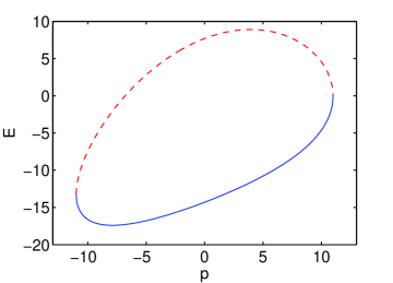
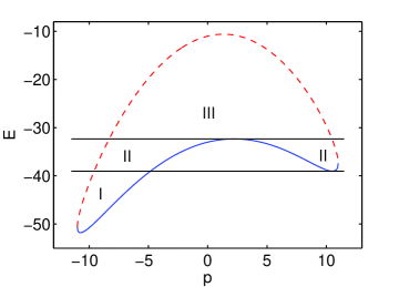
Figure 5: (Color online) The potentials $U_{-}(p)$ (—) and $U_{+}(p)$ (- -), for $N=10$ particles, $v=1$ and $\varepsilon=0.6$ in the subcritical ($g=-0.6/N_{s}$, top) and supercritical ($g=-4/N_{s}$, bottom) region, with $\hbar=1$.

III.2 Energy quantization

In the case of a single classically accessible region, where there are two real turning points for any energy $E$, the semiclassical quantization condition is given by

$$S(E)=h(n+{\textstyle\frac{1}{2}})\ ,\quad n=0,\,1,\,\ldots,N\,.$$ (8)

This simple case is always met in the subcritical region $|g|<v/N_{s}$. A numerical solution of (8) determines the semiclassical energies $E_{n}$, $n=0,\ldots,N$, where the total available phase space area, $0\leq S(E)\leq hN_{s}$, restricts the number of semiclassical eigenvalues to $N_{s}$, exactly as the quantum ones. The resulting semiclassical eigenvalues shown in Fig. 2 for $N=10$ particles ($g=-0.5/N_{s}$, $v=1$, $\hbar=1$) are in excellent agreement with the exact quantum ones.

It should be pointed out, that in the noninteracting case, $g=0$, the action $S(E)$ is a linear function of the energy $E$, and the semiclassical eigenvalues agree with the exact ones

$$E_{n}=\sqrt{\varepsilon^{2}+v^{2}}(2n-N)\ ,\quad n=0,\,1,\,\ldots,N\,.$$ (9)

This can be easily understood by recognizing that in this case the Hamiltonian (1) describes nothing but a system of two coupled harmonic oscillators, which can be transformed to two uncoupled ones by introducing normal coordinates. It may also be of interest to note that (for $g=0$ and $N=2$ or $3$) the classical analog (5) to the quantum Hamiltonian (1) has been suggested many years ago by Miller and coworkers and applied in a semiclassical description of electronic transitions in atom-molecule collisions Mill78 ; Meye79 .

The supercritical region $|g|>v/N_{s}$ is more complicated. Here the energy surface has two minima, hence the potential function $U_{-}(p)$ has two minima as well, separated by a potential barrier. In this case one has to distinguish different regions of the energy. For energies below the upper minimum (region I in Fig. 5), the quantization can be carried out like in the subcritical case by equation (8). For energies between the upper minimum and the barrier $E_{\rm barr}$ (regions II in Fig. 5), there are four real turning points $p^{(l)}_{-}<p^{(l)}_{+}<p^{(r)}_{-}<p^{(r)}_{+}$. In this case one has to consider tunneling through the barrier. The semiclassical quantization condition can be achieved by a more elaborate expression Chil74 (see also Froe72 ; Chil91 ):

$$\sqrt{1+\kappa^{2}}\,\cos(S_{l}+S_{r}-S_{\phi})=-\kappa\,\cos(S_{r}-S_{r}+S_{\theta})$$ (10)

where $S_{l}$ and $S_{r}$ are the action integrals in the left resp. right region in Fig. 5 (note that also here one has to distinguish the different cases a) and c)). The term

$$\kappa={\rm e}^{-\pi S_{\epsilon}}\ ,\ S_{\epsilon}=\frac{1}{\pi}\int_{p_{+}^{(l)}}^{p_{-}^{(r)}}|q(p,E)|\,{\rm d}p$$ (11)

accounts for tunneling through the barrier,

$$S_{\phi}=\arg\Gamma({\textstyle\frac{1}{2}}+{\rm i}S_{\epsilon})-S_{\epsilon}\,\log|S_{\epsilon}|+S_{\epsilon}$$ (12)

is a phase correction, and $S_{\theta}=0$ below the barrier. Deep below the barrier, tunneling can be neglected and the simple semiclassical single well quantization is recovered (see also Wu06 ).

Above the barrier, the inner turning points $p_{+}^{(l)}$, $p_{-}^{(r)}$ turn into a complex conjugate pair and different continuations of the semiclassical quantization have been suggested Chil74 ; Froe72 ; Chil91 . Following Chil74 we replace these turning points by the momentum at the barrier $p_{\rm barr}$ in the formulas for $S_{l,r}$, modify the tunneling integral $S_{\epsilon}$ as

$$S_{\epsilon}=\frac{{\rm i}}{2}(p_{-}^{(r)}-p_{+}^{(l)})-\frac{{\rm i}}{\pi}\int_{p_{+}^{(l)}}^{p_{-}^{(r)}}q(p,E)\,{\rm d}p$$ (13)

and introduce a non-vanishing action integral

$$S_{\theta}=\int_{p_{+}^{(l)}}^{p_{\rm barr}}q(p,E)\,{\rm d}p+\int_{p_{-}^{(r)}}^{p_{\rm barr}}q(p,E)\,{\rm d}p.$$ (14)

The combined semiclassical approximation is continuous if the energy varies across the barrier (from region II to III in Fig. 5) and continuously approaches the simple version with only two turning points $p_{-}^{(l)}$ and $p_{+}^{(r)}$ in region III high above the barrier.

Figure 4 shows the semiclassical many particle energy eigenvalues in dependence on the parameter $\varepsilon$ in the supercritical region for $N=10$ particles ($g=-3/N_{s}$, $v=1$, $\hbar=1$). Also here one observes an almost precise agreement with the exact eigenvalues and the net of avoided level crossings in all details. In particular the level distances at the avoided crossings are reproduced and allow furthermore a direct semiclassical evaluation. Figure 6 shows both exact and semiclassical eigenvalues in dependence on $\varepsilon$ for subcritical interaction for only $N=2$ particles. Even for that small particle number the semiclassical eigenvalues approximate the exact ones quite well. The deviation between the semiclassical and exact quantum eigenvalues decreases with increasing particle number $N$.

For a more quantitative comparison, the exact and semiclassical eigenvalues are listed in Table 1 for $N=20$ particles and selected $\varepsilon$-values. Here the relative error is only about $5\cdot 10^{-4}$.

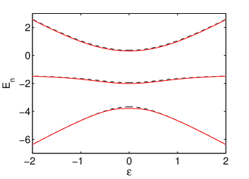
Figure 6: (Color online) Exact (- -), $E_{n}$ and semiclassical (—) many particle energies, $E_{n}^{sc}$, as a function of the onsite energy $\varepsilon$ in the subcritical region ($g=-0.9/N_{s}$) for $v=1$ and $N=2$ particles ($\hbar=1$).

$\varepsilon=0$		$\varepsilon=0.5$		$\varepsilon=1.0$		$\varepsilon=1.5$
$E_{n}$	$E_{n}^{sc}$	$E_{n}$	$E_{n}^{sc}$	$E_{n}$	$E_{n}^{sc}$	$E_{n}$	$E_{n}^{sc}$
12.481	12.469	11.823	11.811	9.859	9.846	6.618	6.600
16.354	16.342	15.692	15.679	13.715	13.702	10.458	10.440
20.097	20.085	19.429	19.417	17.437	17.424	14.161	14.143
23.707	23.695	23.032	23.020	21.021	21.008	17.722	17.703
27.178	27.167	26.496	26.484	24.462	24.449	21.135	21.115
30.508	30.497	29.815	29.804	27.753	27.741	24.391	24.370
33.690	33.679	32.985	32.974	30.888	30.875	27.481	27.458
36.718	36.708	35.997	35.987	33.857	33.844	30.395	30.369
39.585	39.575	38.845	38.835	36.648	36.635	33.115	33.085
42.281	42.272	41.516	41.507	39.246	39.234	35.622	35.583
44.795	44.786	43.999	43.990	41.630	41.618	37.896	37.829
47.111	47.104	46.273	46.265	43.758	43.745	40.090	40.070
49.181	49.176	48.301	48.299	45.649	45.642	43.015	43.023
51.112	51.107	50.031	50.024	46.729	46.739	46.847	46.853
52.193	52.192	51.406	51.406	48.952	48.979	51.439	51.443
54.690	54.687	52.871	52.870	52.760	52.771	56.717	56.720
54.783	54.781	54.680	54.678	57.413	57.419	62.641	62.643
58.828	58.825	56.738	56.750	62.782	62.786	69.187	69.188
58.829	58.826	61.512	61.518	68.813	68.815	76.340	76.341
63.766	63.763	67.009	67.013	75.475	75.477	84.090	84.091
63.766	63.763	73.171	73.173	82.751	82.752	92.432	92.433

Table 1: Exact quantum $E_{n=0...20}$ and semiclassical eigenvalues $E_{n}^{sc}$ for $\varepsilon=0,\,0.5,\,1.0,\,1.5$ for $v=1$ and $N=20$ particles ($\hbar=1$) in the supercritical region ($g=-3/N_{s}$).

III.3 Eigenfunctions

The mean-field approximation allows also a semiclassical construction of the eigenstates $\hat{H}|\Psi_{n}\rangle=E_{n}|\Psi_{n}\rangle$ of the Bose-Hubbard Hamiltonian (1) resp. (2). In the quantum case, the main interest may concentrate on the population imbalance of these states, i.e. the $p$-representation

$$|\Psi_{n}\rangle=\sum_{p=-N:2:N}\Psi_{n}(p)\,|p\rangle\,,$$ (15)

where $p$ runs from $-N$ to $N$ in steps of 2. Based on the (classical) mean-field dynamics, we have to construct a semiclassical approximation in momentum space, which is discussed in some detail in 00mom . The purely classical momentum probability distribution is easily calculated as $w^{cl}(p)=(2T|\partial{\cal H}/\partial q|)^{-1}$, where $T$ is the period of oscillation. Note that the factor 2 arises from the two classical contributions, i.e. the direct path and the path once reflected at the opposite turning point. For our mean-field Hamiltonian (5) this leads to

$$\textstyle w^{cl}(p)=C\Big{[}v^{2}\big{(}N_{s}^{2}-\frac{p^{2}}{\hbar^{2}}\big{)}-\big{(}E^{sc}_{n}-\varepsilon\frac{p}{\hbar}-\frac{g}{2}(N_{s}^{2}+\frac{p^{2}}{\hbar^{2}})\big{)}^{2}\Big{]}^{-\frac{1}{2}}$$ (16)

in the classically allowed region, where $C=1/2T$ takes care of the normalization. The so-called primitive semiclassical wavefunction includes interference of the two classical paths:

$$|\Psi_{n}^{sc}(p)|^{2}=2\,|w_{c}(p)|\,\cos^{2}\big{(}S(p)/\hbar-\pi/4\big{)}$$ (17)

where $S(p)=S(p,E^{sc}_{n})$ is the classical action for an energy equal to the semiclassical eigenenergy $E^{sc}_{n}$ of state number $n$, i.e. the oriented momentum-integral over $q(p)=q(p,E^{sc}_{n})$

$$S(p)=-\int_{p_{-}}^{p}{q(p^{\prime})\,dp^{\prime}}+\frac{\pi}{2}\big{(}p-p_{-}\big{)},$$ (18)

if $p_{-}$ lies on the lower potential curve $U_{-}$ or

$$S(p)=\int_{p_{-}}^{p}{q(p^{\prime})\,dp^{\prime}}.$$ (19)

if $p_{-}$ lies on $U_{+}$. In the classical forbidden region $q(p)$ is complex valued and we can use the usual complex continuation Chil91

$$|\Psi_{n}^{sc}(p)|^{2}=\frac{1}{2}\left|w^{cl}_{n}(p)\exp{(-2{\rm i}S(p)/\hbar)}\right|;$$ (20)

where

$$S(p)=\left\{\begin{matrix}\mp\int_{p}^{p_{-}}{q(p)\,dp},\qquad p<p_{-},\ p_{-}\ \text{on}\ U_{\pm}\\[5.69054pt] \mp\int_{p_{+}}^{p}{q(p)\,dp},\qquad p>p_{+},\ p_{+}\ \text{on}\ U_{\pm}\end{matrix}\right.\,.$$ (21)

Note that these distributions should be renormalized to unity.

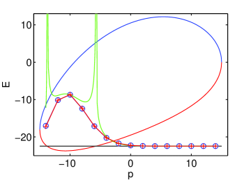
Figure 7: (Color online) Momentum “potentials” $U_{\pm}(p)$ and – plotted at the energy $E_{n}$ – exact (blue circles), primitive semiclassical (green) and uniform semiclassical (red crosses) wavefunctions $|\Psi_{n}(p)|^{2}$ of the lowest eigenstate $n=0$ for $N=14$ particles ($g=-0.6/N_{s}$, $\varepsilon=0.6$, $v=1$ and $\hbar=1$). The solid lines are drawn to guide the eye.

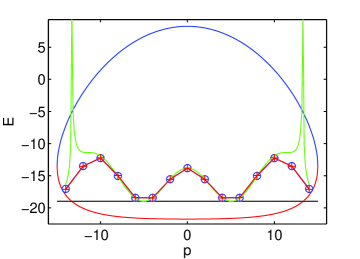
Figure 8: (Color online) Momentum “potentials” $U_{\pm}(p)$ and – plotted at the energy $E_{n}$ – exact (blue circles), primitive semiclassical (green) and uniform semiclassical (red crosses) wavefunctions $|\Psi_{n}(p)|^{2}$ of eigenstate $n=2$ for $N=14$ particles ($g=-0.9/N_{s}$, $\varepsilon=0$, $v=1$ and $\hbar=1$). The solid lines are drawn to guide the eye.

The divergence at the classical turning points $p_{\pm}$ is finally cured by a uniform semiclassical approximation (see e.g. Chil91 ). Here the different turning point scenarios discussed above must be distinguished.In the following we only state the result if $p_{\pm}$ both lie on the lower potential curve $U_{-}(p)$. A mapping onto harmonic oscillator wave functions then yields Chil91

$$|\Psi_{n}^{sc}(p)|^{2}\sim\left|w^{cl}_{n}(p)\sqrt{2n+1-\xi^{2}}\right|\text{H}_{n}(\xi)^{2}\exp{(-\xi^{2})}$$ (22)

where H_n denotes the Hermite polynomial of $n$th order and $\xi$ is determined by

$$\frac{1}{2}\xi\,\sqrt{\xi_{0}^{2}-\xi^{2}}+\frac{1}{2}\xi_{0}^{2}\Big{(}\frac{\pi}{2}+\arcsin{\big{(}\frac{\xi}{\xi_{0}}\big{)}}\Big{)}=S(p)$$ (23)

with $\xi_{0}=\sqrt{2n+1}$.

Up to now, the semiclassical momentum variable $p$ could be treated as continuous in the mean-field approximation, whereas in the quantum system, $p$ is a discrete variable, $p=-N,-N+2,\ldots,+N$. Semiclassically, this is a consequence of the even symmetry and the $\pi$-periodicity of the mean-field Hamiltonian (5) in the coordinate $q$. As in Fourier transformation, this allows only even or odd integer values of $p$.

The final uniform semiclassical wave functions in momentum space are therefore given by (22) at $p=-N,\ldots,N$, normalized as $\sum_{p=-N:2:N}|\Psi_{n}^{sc}(p)|^{2}=1$.

Figures 7 and 8 show a comparison of the primitive semiclassical approximation (normalized to fit the central maximum) and the uniform one with exact quantum results, both in the subcritical region for $N=14$ particles. Shown is the ground state $n=0$ for a biased Bose-Hubbard model ($\varepsilon=0.6$) and the third excited state $n=2$ for a symmetric one ($\varepsilon=0$). As expected, the quantum distributions mainly populate the classically allowed region inside the “potential” curves $U_{\pm}(p)$ and are very well approximated by the primitive semiclassical distributions. In particular, the uniform approximation is almost indistinguishable from the exact values.

IV Conclusion

It is demonstrated for a two-mode Bose-Hubbard model, that the mean-field approximation can be used to reconstruct approximately the individual eigenvalues in a semiclassical Bohr-Sommerfeld (or EBK) manner with astounding accuracy even for a small number of particles. The same holds for the primitive semiclassical approximation of corresponding eigenstates which was shown for the subcritical case. Furthermore the possibility of a uniform approximation was demonstrated for a special case.

For the two-mode Bose-Hubbard system considered here, the classical description provided by the mean-field model has one degree of freedom and is therefore integrable. For three and more modes, the classical dynamics is chaotic (see, e.g., the studies of the three-mode system Moss06 ; 05level3 or tilted optical lattices Thom03 ). Chaoticity also appears in periodically driven two-mode systems Holt01a ; 07kicked or the related kicked tops Haak01 . A semiclassical description of the quasienergy spectrum in these cases is a challenge for future studies.

Finally it should be noted that the semiclassical analysis used in the present paper is based on well-known results which allow, e.g., a straightforward treatment of tunneling corrections. Basically these theories are, however, valid for a flat phase space. More recent developments directly address semiclassical quantization of spin Hamiltonians with a compact phase space (see, e.g., Shan80 ; Garg04 ; Nova05 and references given there). This research is, however, still in progress and applications to Hamiltonians like (2) including tunneling corrections will be the topic of future investigations.

- (1) A. Vardi and J. R. Anglin, Phys. Rev. Lett. 86, 568 (2001).
- (2) J. R. Anglin and A.Vardi, Phys. Rev. A 64, 013605 (2001).
- (3) K. W. Mahmud, H. Perry, and W. P. Reinhardt, Phys. Rev. A 71, 023615 (2005).
- (4) S. Mossmann and C. Jung, Phys. Rev. A 74, 033601 (2006).
- (5) D. Witthaut, E. M. Graefe, and H. J. Korsch, Phys. Rev. A 73, 063609 (2006).
- (6) Biao Wu and Jie Liu, Phys. Rev. Lett. 96, 020405 (2006).
- (7) For a bibliography on the discrete self-trapping equation and its quantized version see http://www.ma.hw.ac.uk/chris/dst/
- (8) M. Enz and R. Schilling, J. Phys. A 19, 1765 (1986); A 19, L711 (1986).
- (9) G. Scharf, W. F. Wreszinski, and J. L. van Hemmen, J. Phys. A 20, 4309 (1987).
- (10) L. Bernstein, J. C. Eilbeck, and A. C. Scott, Nonlinearity 3, 293 (1990).
- (11) D. A. Garanin, J. Phys. A 24, L61 (1991).
- (12) R. Franzosi and V. Penna, Phys. Rev. A 63, 043609 (2001).
- (13) M. Brack and R. K. Bhaduri, Semiclassical Physics (Addison-Wesley, 1997).
- (14) Note that the energy spectrum stays the same if the sign of is altered. If the sign of is altered it is turned upside down. This does not change the subsequent approach in principle.
- (15) M. J. Ablowitz, B. Prinari, and A. D. Trubatch, Discrete and Continuous Nonlinear Schrödinger Systems (Cambridge University Press, Cambridge, 2004).
- (16) L. D. Faddeev and L. A. Takhtajan, Hamiltonian Methods in the Theory of Solitons (Springer, Berlin, Heidelberg, 1987).
- (17) A. Heslot, Phys. Rev. D 31, 1341 (1985).
- (18) S. Aubry, S. Flach, K. Kladko, and E. Olbrich, Phys. Rev. Lett. 76, 1607 (1996).
- (19) G. J. Milburn, J. Corney, E. M. Wright, and D. F. Walls, Phys. Rev. A 55, 4318 (1997).
- (20) M. Holthaus and S. Stenholm, Eur. Phys. J. B 20, 451 (2001).
- (21) Z. P. Karkuszewski, K. Sacha, and A. Smerzi, Eur. Phys. J. D 21, 251 (2002).
- (22) P. Buonsante, R. Franzosi, and V. Penna, J. Phys. B 37, S229 (2004).
- (23) P. A. Braun, Rev. Mod. Phys. 65, 115 (1993).
- (24) F. Haake, Quantum Signatures of Chaos (Springer, Berlin, Heidelberg, New York, 2001).
- (25) W. H. Miller and C. W. McCurdy, J. Chem. Phys. 69, 5163 (1978).
- (26) H. D. Meyer and W. H. Miller, J. Chem. Phys. 70, 3214 (1979); 71, 2156 (1979).
- (27) M. S. Child, J. Molec. Spec. 53, 280 (1974).
- (28) N. Fröman, P. O. Fröman, U. Myhrman, and R. Paulsson, Ann. Phys. (N.Y.) 74, 314 (1972).
- (29) M. S. Child, Semiclassical mechanics with molecular applications (Oxford University Press, Oxford, 1991).
- (30) H. J. Korsch and B. Schellhaaß, Eur. J. Phys. 21, 63 (2000); 21, 73 (2000).
- (31) E. M. Graefe, H. J. Korsch, and D. Witthaut, Phys. Rev. A 73, 013617 (2006).
- (32) Q. Thommen, J. C. Garreau, and V. Zehnlé, Phys. Rev. Lett. 91, 210405 (2003).
- (33) M. P. Strzys, E. M. Graefe, and H. J. Korsch, preprint: quant-ph/0703148 (2007).
- (34) R. Shankar, Phys. Rev. Lett. 45, 1088 (1980).
- (35) A. Garg and M. Stone, Phys. Rev. Lett. 92, 010401 (2004).
- (36) M. Novaea and A. M. de Aguiar, Phys. Rev. A 71, 012104 (2005).