Stationary entanglement between two movable mirrors in a classically driven Fabry-Perot cavity

Abstract

We consider a Fabry-Perot cavity made by two moving mirrors and driven by an intense classical laser field. We show that stationary entanglement between two vibrational modes of the mirrors, with effective mass of the order of micrograms, can be generated by means of radiation pressure. The resulting entanglement is however quite fragile with respect to temperature.

Keywords: Mechanical effects of light, Entanglement

1 Introduction

Quantum entanglement is a physical phenomenon in which the quantum states of two or more systems can only be described with reference to each other. It is now intensively studied not just because of its critical role in setting the boundary between classical and quantum world, but also because it is an important physical resource that allows performing communication and computation tasks with an efficiency which is not achievable classically [1]. In particular, both from a conceptual and a practical point of view, it is important to investigate under which conditions entanglement between macroscopic objects, each containing a large number of the constituents, can arise. Entanglement between two atomic ensembles has been successfully demonstrated in Ref. [2] by sending pulses of coherent light through two atomic vapor cells. More recently Ref. [3] has shown spectroscopic evidence for the creation of entangled macroscopic quantum states in two current-biased Josephson-junction qubits coupled by a capacitor. The interest has been also extended to micro- and nano-mechanical oscillators, which have been shown to be highly controllable [4] and represent natural candidates for quantum limited measurements and for testing decoherence theories [5]. Recent proposals suggested to entangle a nano-mechanical oscillator with a Cooper-pair box [6], arrays of nano-mechanical oscillators [7], two mirrors of an optical ring cavity [8], or two mirrors of two different cavities illuminated with entangled light beams [9]. These two latter proposals employed the optomechanical coupling provided by radiation pressure, which has been demonstrated to provide a useful tool to manipulate the quantum state of light [10, 11, 12, 13, 14, 15, 16].

Here we study the simplest scheme in which one can test the entangling capabilities of radiation pressure, that is, a linear Fabry-Perot cavity with two vibrating mirrors (see Fig. 1). This system corresponds to a simplified version of the system of Ref. [17], where a double-cavity set-up formed by a linear Fabry-Perot cavity and a “folded” ring cavity is considered. Similarly to what has been done in Ref. [17], we determine here the exact steady state of the system and show that if the cavity is appropriately detuned, one can generate stationary entanglement between macroscopic oscillators (effective mass $\sim 100$ ng). As it will be discussed below, the main advantages of the present scheme with respect to that of Ref. [17] are its simplicity and the fact that steady-state entanglement is achievable even with purely classical driving light, while Ref. [17] considered the limiting case of large mechanical frequencies where entanglement can be generated only by injecting nonclassical squeezed light into the two cavities.

The paper is organized as follows. In Section II we describe the dynamics of the system in terms of quantum Langevin equations. In Section III we solve the dynamics and derive the correlation matrix of the steady state of the system. In Section IV we quantify the mechanical entanglement in terms of the logarithmic negativity, while in Section V we compare the present scheme with other recent proposals for the generation of mechanical entanglement and discuss how one can detect it. Section VI is for concluding remarks.

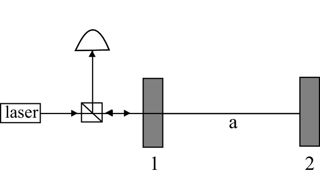
Figure 1: Schematic description of the system under study. The cavity (with mode $a$) is driven by a laser, and the vibrating mirrors 1 and 2 are the ones we want to entangle.

2 The system

We consider an optical Fabry-Perot cavity in which both mirrors can move under the effect of the radiation pressure force (see Fig. 1). The motion of each mirror is described by the excitation of several degrees of freedom which have different resonant frequencies. However, a single frequency mode can be considered for each mirror when a bandpass filter in the detection scheme is used [19] and mode-mode coupling is negligible. Therefore we will consider a single mechanical mode for each mirror, modeled as an harmonic oscillator with frequency $\Omega_{k}$ and effective mass $M_{k}$, $k=1,2$, so that the mechanical Hamiltonian of the mirrors is given by

$$H_{m}=\frac{P_{1}^{2}}{2M_{1}}+\frac{P_{2}^{2}}{2M_{2}}+\frac{1}{2}M_{1}\Omega_{1}^{2}Q_{1}^{2}+\frac{1}{2}M_{2}\Omega_{2}^{2}P_{2}^{2},$$ (1)

with $[Q_{k},P_{j}]=i\hbar\delta_{kj}$. In the adiabatic limit in which the mirror frequencies are much smaller than the cavity free spectral range $c/2L$ ($L$ is the cavity length in the absence of the intracavity field) [20], one can focus on one cavity mode only because photon scattering into other modes can be neglected, and one has the following total Hamiltonian

$$H=H_{m}+\hbar\omega_{c}a^{\dagger}a+\hbar\frac{\omega_{c}}{L}a^{\dagger}a(Q_{1}-Q_{2})+\imath\hbar E(e^{-\imath\omega_{L}t}a^{{\dagger}}-e^{\imath\omega_{L}t}a),$$ (2)

where $a$ and $a^{{\dagger}}$ ($[a,a^{{\dagger}}]=1$) are the annihilation and creation operators of the cavity mode with frequency $\omega_{c}$ and decay rate $\kappa$, and the last two terms in Eq. (2) describe the driving laser with frequency $\omega_{L}$ and $E$ is related to the input laser power $P$ by $|E|=\sqrt{2P\kappa/\hbar\omega_{L}}$. In general the mirror potential is also determined by the additional static Casimir term $V_{Cas}=-\hbar\pi/\left[24(Q_{2}-Q_{1}+L)\right]$ [20], which however is negligible for typical optical cavities with $L\sim 1$ cm and mirrors with effective masses in the $\mu$g–ng range.

The full dynamics of the system is described by a set of nonlinear Langevin equations, including the effects of vacuum radiation noise and the quantum Brownian noise acting on the mirrors. In the interaction picture with respect to $\hbar\omega_{L}a^{{\dagger}}a$

$$\dot{a}=-(\kappa+i\Delta_{0})a-i\frac{\omega_{c}}{L}a(Q_{1}-Q_{2})+E+\sqrt{2\kappa_{1}}a^{in},$$ (3)

$$\dot{Q}_{k}=P_{k}/M_{k},\;\;k=1,2,$$ (4)

$$\dot{P}_{k}=-M_{k}\Omega_{k}^{2}Q_{k}-\gamma_{k}P_{k}+(-1)^{k}\hbar\frac{\omega_{c}}{L}a^{\dagger}a+M_{k}W_{k}\;\;k=1,2,$$ (5)

where $\Delta_{0}=\omega_{c}-\omega_{L}$ and $\gamma_{k}$ is the mechanical damping rate of mirror $k$. We have introduced the radiation input noise $a^{in}(t)$, whose only nonzero correlation function is [21]

$$\langle a^{in}(t)a^{in,{\dagger}}(t^{\prime})\rangle=\delta(t-t^{\prime}),$$ (6)

and the Hermitian Brownian noise operators $W_{j}(t)$, with zero mean value and possessing the following correlation functions [22, 23]

$$\left\langle W_{i}(t)W_{j}(t^{\prime})\right\rangle=\delta_{ij}\frac{\hbar\gamma_{j}}{M_{j}}\int_{-\infty}^{\infty}\frac{d\omega}{2\pi}e^{-i\omega(t-t^{\prime})}\omega\left[\coth\left(\frac{\hbar\omega}{2k_{B}T}\right)+1\right],$$ (7)

where $k_{B}$ is the Boltzmann constant and $T$ is the equilibrium temperature, assumed to be equal for the two mirrors.

We are interested in the dynamics of the quantum fluctuations around the steady state of the system. We can rewrite each Heisenberg operator as a c-number steady state value plus an additional fluctuation operator with zero mean value, $a=\alpha_{s}+\delta a$, $Q_{k}=Q_{k}^{s}+\delta Q_{k}$, $P_{k}=P_{k}^{s}+\delta P_{k}$. Inserting these expressions into the Langevin equations of Eqs. (3), these latter decouple into a set of nonlinear algebraic equations for the steady state values and a set of quantum Langevin equations for the fluctuation operators. The steady state values are given by $P_{k}^{s}=0$, ($k=1,2$), $Q_{k}^{s}=(-1)^{k}(\hbar\omega_{c}/M_{k}\Omega_{k}^{2}L)|\alpha_{s}|^{2}$, $\alpha_{s}=E/(\kappa+i\Delta)$, where the latter equation is in fact a nonlinear equation determining the stationary intracavity field amplitude $\alpha_{s}$, because the effective cavity detuning $\Delta$, including radiation pressure effects, is given by

$$\Delta=\Delta_{0}+\frac{\omega_{c}}{L}\left(Q_{1}^{s}-Q_{2}^{s}\right)$$ (8)

$$=\Delta_{0}-\hbar\left(\frac{\omega_{c}}{L}\right)^{2}|\alpha_{s}|^{2}\left(\frac{1}{M_{1}\Omega_{1}^{2}}+\frac{1}{M_{2}\Omega_{2}^{2}}\right).$$ (9)

The exact quantum Langevin equations for the fluctuations are

$$\delta\dot{a}=-(\kappa+i\Delta)\delta a-i\frac{\omega_{c}}{L}\left(\alpha_{s}+\delta a\right)\left(\delta Q_{1}-\delta Q_{2}\right)+\sqrt{2\kappa}a^{in},$$ (10)

$$\delta\dot{Q_{k}}=\delta P_{k}/M_{k}\;\;k=1,2,$$ (11)

$$\delta\dot{P_{k}}=-M_{k}\Omega_{k}^{2}\delta Q_{k}-\gamma_{k}\delta P_{k}+(-1)^{k}\hbar\frac{\omega_{c}}{L}\left(\alpha_{s}\delta a^{\dagger}+\alpha_{s}^{*}\delta a\right)$$

$$+\delta a^{\dagger}\delta a+M_{k}W_{k}\;\;k=1,2.$$ (12)

From a physical point of view the strong driving regime is the most relevant one. In this regime, the intracavity amplitude is very large, $|\alpha_{s}|\gg 1$, and, as shown by Eqs. (10) and (12), one has a large effective optomechanical coupling constant $\alpha_{s}\omega_{c}/L$ between the field quadrature fluctuations and the oscillator. When $|\alpha_{s}|\gg 1$, one can safely neglect the cavity field fluctuation operator $\delta a$ with respect to $\alpha_{s}$ in Eqs. (10) and (12) and consider linearized Langevin equations. Notice that this amounts to linearize only with respect to the cavity mode and not with respect to the mechanical oscillator, whose operators appear linearly in the dynamical equations from the beginning and therefore are not approximated in the linearized treatment.

It is evident that the cavity mode is coupled only to the relative motion of the two mirrors and it is therefore convenient to rewrite the above equations in terms of the fluctuations of the relative and center-of-mass coordinates, i.e.,

$$\delta Q_{cm} = \frac{M_{1}}{M_{T}}\delta Q_{1}+\frac{M_{2}}{M_{T}}\delta Q_{2},\hskip 14.22636pt\delta P_{cm}=\delta P_{1}+\delta P_{2},$$ (13)

$$\delta Q_{r} = \delta Q_{2}-\delta Q_{1},\hskip 14.22636pt\frac{\delta P_{r}}{\mu}=\frac{\delta P_{2}}{M_{2}}-\frac{\delta P_{1}}{M_{1}},$$ (14)

where $M_{T}=M_{1}+M_{2}$ and $\mu=M_{1}M_{2}/M_{T}$ are the total and reduced mass of the two oscillators. The linearized Langevin equations for these coordinates are

$$\delta\dot{a} = -(\kappa+i\Delta)\delta a+i\frac{\omega_{c}}{L}\alpha_{s}\delta Q_{r}+\sqrt{2\kappa}a^{in},$$ (15)

$$\delta\dot{Q}_{r} = \delta P_{r}/\mu,$$ (16)

$$\delta\dot{P}_{r} = -\mu\Omega_{r}^{2}\delta Q_{r}-\gamma_{r}\delta P_{r}-\mu\left(\Omega_{2}^{2}-\Omega_{1}^{2}\right)\delta Q_{cm}$$ (17)

$$-\frac{\mu}{M_{T}}\left(\gamma_{2}-\gamma_{1}\right)\delta P_{cm}+\hbar\frac{\omega_{c}}{L}\left(\alpha_{s}^{*}\delta a+\alpha_{s}\delta a^{\dagger}\right)+\mu W_{r},$$

$$\delta\dot{Q}_{cm} = \delta P_{cm}/M_{T},$$ (18)

$$\delta\dot{P}_{cm} = -M_{T}\Omega_{cm}^{2}\delta Q_{cm}-\gamma_{cm}\delta P_{cm}$$ (19)

$$-\mu\left(\Omega_{2}^{2}-\Omega_{1}^{2}\right)\delta Q_{r}-\left(\gamma_{2}-\gamma_{1}\right)\delta P_{r}+M_{T}W_{cm},$$

where we have defined the center-of-mass frequency $\Omega_{cm}^{2}=\left(M_{1}\Omega_{1}^{2}+M_{2}\Omega_{2}^{2}\right)/M_{T}$, damping rate $\gamma_{cm}=\left(M_{1}\gamma_{1}+M_{2}\gamma_{2}\right)/M_{T}$, and Brownian noise $W_{cm}=\left(M_{1}W_{1}+M_{2}W_{2}\right)/M_{T}$, and also the relative motion frequency $\Omega_{r}^{2}=\left(M_{2}\Omega_{1}^{2}+M_{1}\Omega_{2}^{2}\right)/M_{T}$, damping rate $\gamma_{r}=\left(M_{2}\gamma_{1}+M_{1}\gamma_{2}\right)/M_{T}$ and Brownian noise $W_{r}=W_{2}-W_{1}$. Thanks to these definitions, the center-of-mass and relative motion Brownian noise possess correlation functions analogous to those of Eq. (7), with the corresponding damping rate and mass. The two noises are however correlated in general, because

$$\left\langle W_{cm}(t)W_{r}(t^{\prime})\right\rangle=\left\langle W_{r}(t)W_{cm}(t^{\prime})\right\rangle$$

$$=\frac{\hbar(\gamma_{2}-\gamma_{1})}{M_{T}}\int_{-\infty}^{\infty}\frac{d\omega}{2\pi}e^{-i\omega(t-t^{\prime})}\omega\left[\coth\left(\frac{\hbar\omega}{2k_{B}T}\right)+1\right].$$ (20)

The above equations show that, even though the cavity mode directly interacts only with the relative motion, the three modes are all coupled because of the center-of-mass–relative-motion coupling, which is present whenever $\Omega_{1}\neq\Omega_{2}$ or $\gamma_{1}\neq\gamma_{2}$.

2.1 Equal frequencies and damping rates

The dynamics considerably simplify when $\Omega_{1}=\Omega_{2}=\Omega$ and $\gamma_{1}=\gamma_{2}=\gamma$. In fact, in such a case $\Omega_{cm}=\Omega_{r}=\Omega$ and $\gamma_{cm}=\gamma_{r}=\gamma$ and the center-of-mass motion fully decouples from the cavity mode and the relative motion, even if the masses are different. The center-of-mass becomes an isolated quantum oscillator with mass $M_{T}$ and subject to quantum Brownian noise, i.e.,

$$\delta\dot{Q}_{cm}=\delta P_{cm}/M_{T},$$ (21)

$$\delta\dot{P}_{cm}=-M_{T}\Omega^{2}\delta Q_{cm}-\gamma\delta P_{cm}+M_{T}W_{cm},$$ (22)

while the relative position of the two mirrors and the linearized fluctuations of the cavity mode form a system of two interacting modes described by the following linear Langevin equations

$$\delta\dot{Q}_{r}=\delta P_{r}/\mu,$$ (23)

$$\delta\dot{P}_{r}=-\mu\Omega^{2}\delta Q_{r}-\gamma\delta P_{r}+\frac{\sqrt{2}\hbar\omega_{c}\alpha_{s}}{L}X+\mu W_{r},$$ (24)

$$\dot{X}=-\kappa X+\Delta Y+\sqrt{2\kappa}X^{in},$$ (25)

$$\dot{Y}=-\kappa Y-\Delta X+\frac{\sqrt{2}\omega_{c}\alpha_{s}}{L}\delta Q_{r}+\sqrt{2\kappa}Y^{in},$$ (26)

where we have chosen the phase reference of the cavity field so that $\alpha_{s}$ is real, we have defined the cavity field quadratures $X\equiv(\delta a+\delta a^{{\dagger}})/\sqrt{2}$ and $Y\equiv(\delta a-\delta a^{{\dagger}})/i\sqrt{2}$, and the corresponding Hermitian input noise operators $X^{in}\equiv(a^{in}+a^{in,{\dagger}})/\sqrt{2}$ and $Y^{in}\equiv(a^{in}-a^{in,{\dagger}})/i\sqrt{2}$. Notice that Eqs. (23) coincide with the linearized equations of a Fabry-Perot cavity with only one movable mirror with mass $\mu$.

It is convenient to switch to dimensionless dynamical variables for the mechanical oscillators. If we define

$$\delta Q_{k}=\sqrt{\frac{\hbar}{M_{k}\Omega}}q_{k},\hskip 14.22636pt\delta P_{k}=\sqrt{\hbar M_{k}\Omega}p_{k},\;k=1,2,$$ (27)

$$\delta Q_{cm}=\sqrt{\frac{\hbar}{M_{T}\Omega}}q_{cm},\hskip 14.22636pt\delta P_{cm}=\sqrt{\hbar M_{T}\Omega}p_{cm},$$ (28)

$$\delta Q_{r}=\sqrt{\frac{\hbar}{\mu\Omega}}q_{r},\hskip 14.22636pt\delta P_{r}=\sqrt{\hbar\mu\Omega}p_{r},$$ (29)

such that $[q_{j},p_{k}]=i\delta_{jk}$, either for $j,k=1,2$ and for $j,k=r,cm$, definitions (13)-(14) become

$$q_{cm} = r_{1}q_{1}+r_{2}q_{2},\hskip 14.22636ptp_{cm}=r_{1}p_{1}+r_{2}p_{2},$$ (30)

$$q_{r} = r_{1}q_{2}-r_{2}q_{1},\hskip 14.22636ptp_{r}=r_{1}p_{2}-r_{2}p_{1},$$ (31)

where $r_{k}=\sqrt{M_{k}/M_{T}}$, $k=1,2$. The quantum Langevin equations become in terms of these dimensionless continuous variables

$$\dot{q}_{cm}=\Omega p_{cm},$$ (32)

$$\dot{p}_{cm}=-\Omega q_{cm}-\gamma p_{cm}+\xi_{cm},$$ (33)

$$\dot{q}_{r}=\Omega p_{r},$$ (34)

$$\dot{p}_{r}=\Omega q_{r}-\gamma p_{r}+GX+\xi_{r},$$ (35)

$$\dot{X}=-\kappa X+\Delta Y+\sqrt{2\kappa}X^{in},$$ (36)

$$\dot{Y}=-\kappa Y-\Delta X+Gq_{r}+\sqrt{2\kappa}Y^{in},$$ (37)

where we have defined the effective optomechanical coupling constant

$$G=\sqrt{\frac{2\hbar}{\mu\Omega}}\frac{\alpha_{s}\omega_{c}}{L}=\frac{2\omega_{c}}{L}\sqrt{\frac{P\kappa}{\mu\Omega\omega_{L}\left(\kappa^{2}+\Delta^{2}\right)}},$$ (38)

which, being proportional to the square root of the input power, can be made quite large, and the zero-mean scaled Brownian noise operators $\xi_{r}(t)$ and $\xi_{cm}(t)$, with correlation functions

$$\left\langle\xi_{j}(t)\xi_{k}(t^{\prime})\right\rangle=\delta_{jk}\frac{\gamma}{\Omega}\int_{-\infty}^{\infty}\frac{d\omega}{2\pi}e^{-i\omega(t-t^{\prime})}\omega\left[\coth\left(\frac{\hbar\omega}{2k_{B}T}\right)+1\right]\;,$$ (39)

where $j,k=$r,cm.

3 Stationary correlation matrix of the two mirrors

When the three-mode system is stable, it reaches a unique steady state, independently from the initial condition. Since the quantum noises $\xi_{cm}$, $\xi_{r}$, $X^{in}$ and $Y^{in}$ are zero-mean quantum Gaussian noises and the dynamics is linearized, the quantum steady state for the fluctuations is a zero-mean Gaussian state, fully characterized by its $6\times 6$ correlation matrix (CM) $V^{(6)}_{ij}=\langle u_{i}(\infty)u_{j}(\infty)+u_{j}(\infty)u_{i}(\infty)\rangle/2$, where $u^{T}(\infty)=(q_{1}(\infty),p_{1}(\infty),q_{2}(\infty),p_{2}(\infty),X(\infty),Y(\infty))$ is the vector of continuous variables (CV) fluctuation operators at the steady state ($t\to\infty$). We are interested in the stationary reduced state of the two mirrors, which is obtained by tracing out the cavity mode. This state is obviously still Gaussian and fully characterized by the $4\times 4$ matrix $V_{ij}$ formed by the first four rows and columns of $V^{(6)}_{ij}$. The general form of $V$ is quite simple. First of all it is $V_{12}=V_{34}=0$. In fact, since $p_{j}=\dot{q}_{j}/\Omega$, $j=1,2$, it is

$$V_{12}=\frac{\langle q_{1}(\infty)p_{1}(\infty)+p_{1}(\infty)q_{1}(\infty)\rangle}{2}=\frac{1}{2\Omega}\lim_{t\to\infty}\frac{d}{dt}\langle q_{1}^{2}(t)\rangle=0,$$ (40)

and the same happens for $V_{34}$. Moreover, thanks to the decoupling between center-of-mass and relative motion it is $V_{14}=V_{23}=0$, because

$$V_{14}=\frac{\langle q_{1}(\infty)p_{2}(\infty)+p_{2}(\infty)q_{1}(\infty)\rangle}{2}$$

$$=\frac{r_{1}r_{2}}{2}\left[\langle q_{cm}(\infty)p_{cm}(\infty)+p_{cm}(\infty)q_{cm}(\infty)\rangle\right.$$

$$-\left.\langle q_{r}(\infty)p_{r}(\infty)+p_{r}(\infty)q_{r}(\infty)\rangle\right]$$

$$=\frac{r_{1}r_{2}}{2\Omega}\lim_{t\to\infty}\frac{d}{dt}\left[\langle q_{cm}^{2}(t)\rangle-\langle q_{r}^{2}(t)\rangle\right]=0,$$ (41)

and the same happens for $V_{23}$. The final form of $V$ is

$$V=\left(\begin{array}[]{cccc}V_{11}&0&V_{13}&0\\ 0&V_{22}&0&V_{24}\\ V_{13}&0&V_{33}&0\\ 0&V_{24}&0&V_{44}\end{array}\right),$$ (42)

where

$$V_{11} = r_{1}^{2}\langle q_{cm}^{2}\rangle_{st}+r_{2}^{2}\langle q_{r}^{2}\rangle_{st},\hskip 14.22636ptV_{22}=r_{1}^{2}\langle p_{cm}^{2}\rangle_{st}+r_{2}^{2}\langle p_{r}^{2}\rangle_{st},$$ (43)

$$V_{33} = r_{2}^{2}\langle q_{cm}^{2}\rangle_{st}+r_{1}^{2}\langle q_{r}^{2}\rangle_{st},\hskip 14.22636ptV_{44}=r_{2}^{2}\langle p_{cm}^{2}\rangle_{st}+r_{1}^{2}\langle p_{r}^{2}\rangle_{st},$$ (44)

$$V_{13} = r_{1}r_{2}\left(\langle q_{cm}^{2}\rangle_{st}-\langle q_{r}^{2}\rangle_{st}\right),\hskip 14.22636ptV_{24}=r_{1}r_{2}\left(\langle p_{cm}^{2}\rangle_{st}-\langle p_{r}^{2}\rangle_{st}\right),$$ (45)

that is, it depends upon the mass ratios $r_{k}$ and the four stationary variances $\langle u^{2}\rangle_{st}\equiv\lim_{t\to\infty}\langle u^{2}(t)\rangle$, $u=q_{cm},p_{cm},q_{r},p_{r}$.

3.1 Calculation of the stationary variances

The center-of-mass and relative motion stationary variances can be obtained by solving Eqs. (32) and considering the limit $t\to\infty$. Defining the six-dimensional vector of variables $v^{T}(t)=(q_{cm}(t),p_{cm}(t),q_{r}(t),p_{r}(t),X(t),Y(t))$, the vector of noises $n^{T}(t)=(0,\xi_{cm}(t),0,\xi_{r}(t),\sqrt{2\kappa}X^{in}(t),\sqrt{2\kappa}Y^{in}(t))$ and the matrix

$$A=\left(\begin{array}[]{cccccc}0&\Omega&0&0&0&0\\ -\Omega&-\gamma&0&0&0&0\\ 0&0&0&\Omega&0&0\\ 0&0&-\Omega&-\gamma&G&0\\ 0&0&0&0&-\kappa&\Delta\\ 0&0&G&0&-\Delta&-\kappa\end{array}\right),$$ (46)

Eqs. (32) can be rewritten in compact form as $\dot{v}(t)=Av(t)+n(t)$, whose solution is

$$v(t)=M(t)v(0)+\int_{0}^{t}dsM(s)n(t-s),$$ (47)

where $M(t)=\exp\{At\}$. The system is stable and reaches its steady state when all the eigenvalues of $A$ have negative real parts so that $M(\infty)=0$. The stability conditions can be derived by applying the Routh-Hurwitz criterion [26], yielding the following two nontrivial conditions on the system parameters,

$$s_{1}=2\gamma\kappa\left[\Delta^{4}+\Delta^{2}(\gamma^{2}+2\gamma\kappa+2\kappa^{2}-2\Omega^{2})\right.$$ (48)

$$\left.+(\gamma\kappa+\kappa^{2}+\Omega^{2})^{2}\right]+\Omega G^{2}\Delta(\gamma+2\kappa)^{2}>0,$$

$$s_{2}=\Omega\left(\Delta^{2}+\kappa^{2}\right)-G^{2}\Delta>0,$$ (49)

which will be considered to be satisfied from now on. If we consider the variables $v_{j}(t)$, we can construct the stationary correlation matrix

$$C_{ij}=\frac{\langle v_{i}(\infty)v_{j}(\infty)+v_{j}(\infty)v_{i}(\infty)\rangle}{2},$$ (50)

which is the quantity of interest because $C_{11}=\langle q_{cm}^{2}\rangle_{st}$, $C_{22}=\langle p_{cm}^{2}\rangle_{st}$, $C_{33}=\langle q_{r}^{2}\rangle_{st}$, and $C_{44}=\langle p_{r}^{2}\rangle_{st}$. When the system is stable, using Eq. (47) one gets

$$C_{ij}=\sum_{k,l}\int_{0}^{\infty}ds\int_{0}^{\infty}ds^{\prime}M_{ik}(s)M_{jl}(s^{\prime})\Phi_{kl}(s-s^{\prime}),$$ (51)

where $\Phi_{kl}(s-s^{\prime})=\left(\langle n_{k}(s)n_{l}(s^{\prime})+n_{l}(s^{\prime})n_{k}(s)\rangle\right)/2$ is the matrix of the stationary noise correlation functions. Due to Eq. (39), the mirror Brownian noises are not delta-correlated and therefore do not describe in general a Markovian process. However, as we shall see, mechanical entanglement is achievable only using oscillators with a very good mechanical quality factor $\mathcal{Q}=\Omega/\gamma$. In this weak damping limit, $\gamma\to 0$, the quantum Brownian noises $\xi_{r}(t)$ and $\xi_{cm}(t)$ become delta-correlated, [27]

$$\left\langle\xi_{j}(t)\xi_{k}(t^{\prime})+\xi_{k}(t^{\prime})\xi_{j}(t)\right\rangle/2\simeq\delta_{jk}\gamma\left(2\bar{n}+1\right)\delta(t-t^{\prime}),$$ (52)

where $\bar{n}=\left(\exp\{\hbar\Omega/k_{B}T\}-1\right)^{-1}$, is the mean thermal excitation number, and one recovers a Markovian process. Using the definitions of $X_{in}$ and $Y_{in}$ and Eq. (6), we finally get $\Phi_{kl}(s-s^{\prime})=D_{kl}\delta(s-s^{\prime})$, where

$$D=\left(\begin{array}[]{cccc}0&0&0&0\\ 0&\gamma(2\bar{n}+1)&0&0\\ 0&0&\kappa&0\\ 0&0&0&\kappa\end{array}\right).$$ (53)

As a consequence, Eq. (51) becomes

$$C=\int_{0}^{\infty}dsM(s)DM(s)^{T},$$ (54)

which, when the stability conditions are satisfied so that $M(\infty)=0$, is equivalent to the following equation for the CM,

$$AC+CA^{T}=-D.$$ (55)

Eq. (55) is a linear equation for $C$ and it can be straightforwardly solved. The center-of-mass is decoupled from the other two modes and Eq. (55) trivially gives

$$C_{11}=C_{22}=\langle q_{cm}^{2}\rangle_{st}=\langle p_{cm}^{2}\rangle_{st}=\frac{1}{2}+\bar{n}.$$ (56)

The relative motion is instead coupled with the cavity mode and consequently the final expression of the stationary variances are much more involved. One has

$$C_{33} = \langle q_{r}^{2}\rangle_{st}=\frac{1}{2}+b_{q}+d_{q}\bar{n},$$ (57)

$$C_{44} = \langle p_{r}^{2}\rangle_{st}=\frac{1}{2}+b_{p}+d_{p}\bar{n},$$ (58)

where

$$b_{p} = [s_{1}]^{-1}G^{2}\kappa\left\{\Delta^{2}(\gamma+\kappa)+\kappa(\gamma\kappa+\kappa^{2}+\Omega^{2})-\Delta\Omega(\gamma+2\kappa)\right\},$$ (59)

$$d_{p} = 1-[s_{1}]^{-1}2G^{2}\kappa\Omega\Delta(\gamma+2\kappa),$$ (60)

$$b_{q} = [2s_{1}s_{2}]^{-1}G^{2}\left\{2\kappa\left(\Delta^{2}+\kappa^{2}\right)\left\{\left[\Delta^{2}+{\left(\gamma+\kappa\right)}^{2}\right]\left(\kappa\Omega+\gamma\Delta\right)\right.\right.$$

$$+ \left.\left.\Omega^{2}\left(\gamma+\kappa\right)\left(\Omega-2\Delta\right)\right\}\Delta G^{2}\Omega^{2}\left(\gamma+2\kappa\right)\left[\Delta\gamma-\kappa\left(\Omega-2\Delta\right)\right]\right\},$$

$$d_{q} = 1+[s_{1}s_{2}]^{-1}\Delta G^{2}\left[s_{1}-2\gamma\kappa\Omega^{2}\left(\Omega^{2}+2\gamma\kappa+4\kappa^{2}\right)\right.$$ (62)

$$- \left.4\kappa^{2}\Omega^{2}\left(\Delta^{2}+\kappa^{2}\right)\right].$$

4 Conditions for stationary entanglement

Simon’s separability PPT (positive partial transpose) criterion is necessary and sufficient for bipartite Gaussian CV states [24]. It assumes a particularly simple form for the CM of the two mirrors of Eq. (42). In fact, after some algebra, one gets the following necessary and sufficient condition for the presence of mechanical entanglement between the two mirrors in the stationary state,

$$\left[\langle q_{r}^{2}\rangle_{st}\langle p_{cm}^{2}\rangle_{st}-\frac{1}{4}\right]\left[\langle p_{r}^{2}\rangle_{st}\langle q_{cm}^{2}\rangle_{st}-\frac{1}{4}\right]<\left(1-\frac{1}{\eta}\right)$$

$$\times\left[\langle q_{cm}^{2}\rangle_{st}\langle p_{cm}^{2}\rangle_{st}-\frac{1}{4}\right]\left[\langle q_{r}^{2}\rangle_{st}\langle p_{r}^{2}\rangle_{st}-\frac{1}{4}\right],$$ (63)

where we have defined $\eta=4r_{1}^{2}r_{2}^{2}=4\mu/M_{T}$. For very different masses $\eta\to 0$ and the right hand side of Eq. (63) tends to $-\infty$, i.e., the criterion is never satisfied and the mirrors are never entangled. It is evident therefore that stationary entanglement is better achieved for equal mirrors, i.e., $\eta=1$, when the right hand side of Eq. (63) is equal to zero and the necessary and sufficient entanglement condition becomes equivalent to a “product” of sufficient criteria analogous to those derived in [8, 25], that is, $\langle q_{r}^{2}\rangle_{st}\langle p_{cm}^{2}\rangle_{st}<1/4$ or $\langle p_{r}^{2}\rangle_{st}\langle q_{cm}^{2}\rangle_{st}<1/4$. Since the center-of-mass of the two mirror is unaffected by the optomechanical coupling (see Eq. (56)), this means that the two mirror vibrational modes are entangled if and only if their relative motion is sufficiently squeezed, i.e.,

$$\langle q_{r}^{2}\rangle_{st}\;\;{\rm or}\;\;\langle p_{r}^{2}\rangle_{st}<\frac{1}{2(1+2\bar{n})}.$$ (64)

This equation provides an intuitive picture of how the entanglement between the two mirrors is generated by the radiation pressure of the light bouncing between them. If the cavity is strongly driven, the radiation pressure coupling becomes very large and the fluctuations of the mirror relative motion can be significantly squeezed. If such a squeezing is large enough to overcome even the thermal noise acting on the center-of-mass, Eq. (64) guarantees that the two mirrors are entangled. Eq. (64) also points out the main limit of the proposed scheme: the mirrors center-of-mass is not affected by radiation pressure and cannot be squeezed. This suggests that the generated entanglement is not robust against temperature because satisfying Eq. (64) becomes prohibitive at large $\bar{n}$.

One can quantify the stationary mechanical entanglement by considering the logarithmic negativity $E_{\mathcal{N}}$ [28], which in the CV case $E_{\mathcal{N}}$ can be defined as [29]

$$E_{\mathcal{N}}=\max[0,-\ln 2\nu^{-}],$$ (65)

where $\nu^{-}$ is given by

$$\nu^{-}\equiv 2^{-1/2}\left[\Sigma(V)-\left(\Sigma(V)^{2}-4\det V\right)^{1/2}\right]^{1/2},$$ (66)

with $\Sigma(V)\equiv\det N_{1}+\det N_{2}-2\det N_{12}$ and we have used the $2\times 2$ block form of the CM

$$V\equiv\left(\begin{array}[]{cc}N_{1}&N_{12}\\ N_{12}^{T}&N_{2}\end{array}\right).$$ (67)

Therefore, a Gaussian state is entangled if and only if $\nu^{-}<1/2$, which is equivalent to Simon’s necessary and sufficient entanglement criterion for Gaussian states [24] of Eq. (63), and which can be written as $4\det V<\Sigma(V)-1/4$. In the case of the stationary matrix $V$ of Eq. (42), one has

$$\det V=\langle q_{r}^{2}\rangle_{st}\langle p_{r}^{2}\rangle_{st}\langle q_{cm}^{2}\rangle_{st}\langle p_{cm}^{2}\rangle_{st}$$ (68)

$$\Sigma(V)=(1-\eta)\left[\langle q_{r}^{2}\rangle_{st}\langle p_{r}^{2}\rangle_{st}+\langle q_{cm}^{2}\rangle_{st}\langle p_{cm}^{2}\rangle_{st}\right]$$

$$+\eta\left[\langle q_{r}^{2}\rangle_{st}\langle p_{cm}^{2}\rangle_{st}+\langle q_{cm}^{2}\rangle_{st}\langle p_{r}^{2}\rangle_{st}\right].$$ (69)

Therefore, in the most convenient condition for entanglement, i.e., identical mirrors $\Leftrightarrow\eta=1$, one has $\Sigma(V)=\langle q_{r}^{2}\rangle_{st}\langle p_{cm}^{2}\rangle_{st}+\langle q_{cm}^{2}\rangle_{st}\langle p_{r}^{2}\rangle_{st}$, yielding

$$\nu^{-}=\min\left\{\sqrt{\langle q_{r}^{2}\rangle_{st}\langle p_{cm}^{2}\rangle_{st}},\sqrt{\langle q_{cm}^{2}\rangle_{st}\langle p_{r}^{2}\rangle_{st}}\right\},$$ (70)

so that in this case of equal masses, the logarithmic negativity assumes the particularly simple form

$$E_{\mathcal{N}}=\max\left\{0,-\ln\left[2\sqrt{\langle q_{r}^{2}\rangle_{st}\langle p_{cm}^{2}\rangle_{st}}\right],-\ln\left[2\sqrt{\langle q_{cm}^{2}\rangle_{st}\langle p_{r}^{2}\rangle_{st}}\right]\right\}.$$ (71)

Using Eqs. (56)-(58), and (71) one has stationary entanglement if one of the two following conditions is satisfied

$$b_{q}+d_{q}\bar{n}<-\frac{\bar{n}}{2\bar{n}+1},$$ (72)

$$b_{p}+d_{p}\bar{n}<-\frac{\bar{n}}{2\bar{n}+1},$$ (73)

which, as expected, are better satisfied in the zero temperature limit, $\bar{n}\to 0$, since $d_{q},d_{p}\geq 0$ whenever the stability conditions are satisfied (otherwise one could have negative variances at large enough temperatures).

These two equations lead us to the main result of the paper, i.e., it is possible to realize an entangled stationary state of two macroscopic movable mirrors of a classically driven Fabry-Perot cavity. However, such a stationary mechanical entanglement turns out to be fragile with respect to temperature, as it can be easily grasped from Eqs. (72)-(73). This is illustrated in Figs. 2-3, where we have considered a parameter region very close to that of recently performed experiments employing optical Fabry-Perot cavities with at least one micromechanical mirror [11, 12, 13, 14]. Figs. 2-3 refer to the case of an optical cavity of length $L=1$ cm, finesse $\mathcal{F}=1.9\times 10^{5}$, so that $\kappa\simeq 5\times 10^{5}$ s^-1, driven by a laser with wavelength $1064$ nm and power $P=50$ mW. The two identical mechanical oscillators have angular frequency $\Omega/2\pi=10$ MHz, damping rate $\gamma=3\times 10^{5}$ s^-1, and mass $m=100$ ng. Fig. 2 refers to the zero temperature limit and shows that stationary entanglement is present only within a small interval of values of $\Delta$ around $\Delta\simeq\Delta_{opt}$ where

$$\Delta_{opt}=\Omega\frac{\gamma+2\kappa}{2\gamma+2\kappa}.$$ (74)

This value is essentially the optimal value for the detuning for achieving entanglement. This can be understood from the expression of $\langle p_{r}^{2}\rangle_{st}$. In fact, at zero temperature entanglement is obtained when $b_{p}<0$ (see Eq. (73)), which is satisfied when the numerator of Eq. (59) is negative, since $s_{1}>0$ due to stability. This condition is obtained by considering the minimum of the second order polynomial in $\Delta$ in the numerator and by imposing that it is negative. The minimum value of this polynomial is obtained just at $\Delta=\Delta_{opt}$ and it is negative when

$$\gamma\Omega>2\kappa(\gamma+\kappa).$$ (75)

Therefore $\Delta=\Delta_{opt}$ and Eq. (75) are sufficient conditions for achieving entanglement at zero temperature. This parameter regime is the optimal for entanglement because when $\Delta\simeq\Delta_{opt}\simeq\Omega$, $s_{1}$ is also close to its minimum value, implying therefore a large negative value of $b_{p}$ (see Eq. (59)) and also a value of $d_{p}$ very close to zero (see Eq. (60)), which means an improved robustness of entanglement with respect to temperature. In Fig. 3 we study the resistance to thermal effects by plotting $E_{\mathcal{N}}$ evaluated at the optimal detuning, i.e., corresponding to the maximum of Fig. 2, versus temperature. We see that this entanglement vanishes for $T>100$ $\mu$K. This behavior is valid in general, even in parameter regions different from that of Figs. 2, 3: whenever one finds a regime with a nonzero stationary entanglement, this entanglement quickly tends to zero for increasing temperatures. As discussed above (see below Eq. (64)) this is due to the fact that in this simple Fabry-Perot cavity system, the mirror center-of-mass is unaffected by the radiation pressure of the cavity mode and remains at thermal equilibrium. One could achieve a larger and more robust entanglement by adopting the double-cavity setup considered in [17], where the optical mode of the second, “folded” cavity couples just to the center-of-mass of the mirrors of interest, which is then also squeezed, independently from the relative motion. In this latter scheme therefore robustness against temperature is achieved at the price of a much more involved experimental setup.

Eq. (71) shows that mechanical entanglement at zero temperature could be realized as well when $\langle q_{r}^{2}\rangle_{st}<1/2$. However, it is possible to see through numerical calculations that this condition is much more difficult to realize with respect to $\langle p_{r}^{2}\rangle_{st}<1/2$. This fact is not easily seen from the analytical expressions of $b_{q}$ and $d_{q}$ (Eqs. (3.1)-(62)), which are more difficult to analyze with respect to those of $b_{p}$ and $d_{p}$ (Eqs. (59)-(60)).

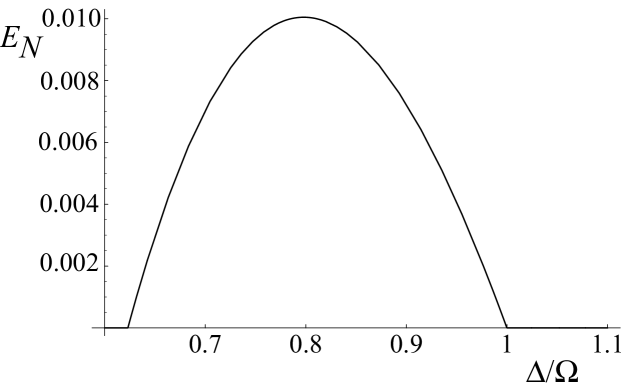
Figure 2: Logarithmic negativity $E_{\mathcal{N}}$ as a function of the normalized detuning $\Delta/\Omega$ in the case of an optical cavity of length $L=1$ cm, finesse $\mathcal{F}=1.9\times 10^{5}$, driven by a laser with wavelength $1064$ nm and power $P=50$ mW. The identical movable mirrors have a frequency $\Omega/2\pi=10$ MHz, damping rate $\gamma=3\times 10^{5}$ s^-1, mass $m=100$ ng and their temperature is $T=0$.

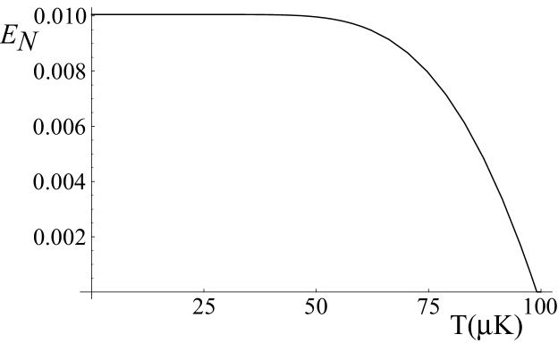
Figure 3: Logarithmic negativity $E_{\mathcal{N}}$ evaluated at $\Delta=\Delta_{opt}\simeq 0.8\Omega$ (see Eq. 74)) as a function of temperature. The other parameter values are the same as in Fig. 2.

5 Comparison with other proposals and experimental detection of the entanglement

It is interesting to compare the present proposal with other recent schemes for entangling two micro-mechanical mirrors, especially with Refs. [8, 9, 17, 18], which are all based on the optomechanical coupling provided by the radiation pressure. Refs. [8, 9, 17] considered the steady state of different systems of driven cavities: Ref. [8] focused on two mirrors of a ring cavity and considered the situation in the frequency domain; Ref. [9] assumed to drive two independent linear cavities with two-mode squeezed light and stationary mechanical entanglement is achieved by transferring the entanglement of the two driving beams to the end-mirrors of the two cavities.

We have already partially compared the present scheme with that of Ref. [17], to which is strongly related. In fact, the double-cavity scheme of Ref. [17] coincides with the single Fabry-Perot cavity scheme considered here when the “folded” cavity of Ref. [17] is not driven. The additional folded cavity couples to the center-of-mass of the two vibrational modes and if it is appropriately driven by squeezed light, it is able to transfer this squeezing to the center-of-mass. This has the advantage of increasing the entanglement and making it more robust against temperature (see Eq. (71)), but this is obtained at the price of a more involved apparatus, requiring the preparation of an additional ring cavity and the use of nonclassical driving. Moreover, Ref. [17] evaluated the stationary state of the two mechanical modes approximately, by considering the resonant case $\Delta=\Omega$ and solving the dynamics of the system only in the limit when $\Omega$ is much larger than the other parameters, $G$, $\kappa$, so that fast terms rotating at frequency $\Omega$ can be neglected in the equations of motion. In this limit, Ref. [17] finds that the steady state of the two mirrors is entangled only if the input field is squeezed, while is never entangled for a classical coherent input. Here we determine the steady state of the system exactly in the Markovian limit of weak mechanical damping and we find that when fast terms rotating at frequency $\Omega$ cannot be neglected, one can entangle the mirror even using classical driving. As expected, it is possible to check that the present exact solution reproduces the results of Ref. [17] in the same limiting conditions (no input squeezing, large mechanical frequency, and no folded cavity). In fact, if we consider $\Delta=\Omega\gg G,\kappa,\gamma$ in Eqs. (59)-(62), one gets

$$b_{p}=b_{q}\simeq 0,$$ (76)

$$d_{p}=d_{q}=\frac{\gamma\left(G^{2}+2\gamma\kappa+4\kappa^{2}\right)}{\left(\gamma+2\kappa\right)\left(G^{2}+2\gamma\kappa\right)},$$ (77)

so that

$$\langle q_{r}^{2}\rangle_{st}=\langle p_{r}^{2}\rangle_{st}=\frac{1}{2}+\bar{n}\frac{\gamma\left(G^{2}+2\gamma\kappa+4\kappa^{2}\right)}{\left(\gamma+2\kappa\right)\left(G^{2}+2\gamma\kappa\right)}\geq\frac{1}{2},$$ (78)

coinciding with Eq. (23) of Ref. [17] in the case of no input squeezing, and implying absence of mechanical entanglement. Therefore we see that the “resonance” condition $\Delta=\Omega$ is very close to the optimal condition for generating mechanical entanglement, and that if one leaves the regime of vary large mechanical frequencies $\Omega\gg G,\kappa,\gamma$, one can achieve stationary mechanical entanglement even without input squeezing. In fact, the parameter regime considered in Figs. 2-3 corresponds to $\Omega\simeq G\gg\kappa\simeq\gamma$.

Another recent proposal employing radiation pressure effects for entangling two vibrating micro-mirrors is Ref. [18], where the radiation pressure of an intense laser field first generates optomechanical entanglement between a mirror vibrational mode and an optical sideband. Such an entanglement is then swapped to two separated micro-mechanical oscillators via homodyne measurements on the optical modes, representing Bell measurements in this continuous variable setting. In this latter proposal, macroscopic mechanical entanglement is generated when the homodyne measurement is performed and it is therefore a transient phenomenon, with a lifetime which is severely limited by the mirror thermal reservoir [18]. In the present scheme, on the contrary, mechanical entanglement has an infinite lifetime because it is generated at the steady state, and therefore its experimental detection becomes much easier.

We also notice that the system studied here is similar to the one considered in Ref. [15], where a Fabry-Perot cavity with only one vibrating mirror is considered. In Ref. [15] a quantum Langevin treatment analogous to the one adopted here is used to quantify the amount of bipartite entanglement between the vibrational mode of the mirror and the intracavity field at the steady state of the system.

We finally discuss the experimental detection of the generated mechanical entanglement. The measurement of $E_{\mathcal{N}}$ at the steady state is quite involved because one has to measure all the ten independent entries of the steady state correlation matrix $V$. This has been recently experimentally realized (see Ref. [30] and references therein) for the case of two entangled optical modes at the output of a parametric oscillator. Instead, one does not have direct access to the vibrational modes and therefore it is not clear how to measure them. However Ref. [15] showed that, apart from additional detection shot noise, the motional state of the mirror can be read from the output of an adjacent Fabry-Perot cavity, formed by the mirror to be detected and another “fixed” (i.e. with large mass) mirror. In fact, it is possible to adjust the parameters of this second cavity so that both position and momentum of the mirror can be experimentally determined by homodyning the cavity output light [15]. In particular, if the readout cavity is driven by a much weaker laser so that its back-action on the mechanical mode can be neglected, its detuning $\Delta_{2}$ is chosen to be equal to the mechanical frequency $\Omega$, and its bandwidth $\kappa_{2}$ is large enough so that the cavity mode adiabatically follows the mirror dynamics, the output of the readout cavity $a_{2}^{out}$ is given by

$$a_{2}^{out}=i\frac{G_{2}}{\sqrt{\kappa_{2}}}b+a_{2}^{in},$$ (79)

where $b$ is the annihilation operator of the vibrational mode, $G_{2}$ is the effective optomechanical coupling of the readout cavity (see Eq. (38)), and $a_{2}^{in}$ is the input noise entering the readout cavity. Therefore using a readout cavity for each mirror, changing the phases of the two local oscillators and measuring the correlations between the two readout cavity output one can then detect all the entries of the correlation matrix $V$ and from them numerically extract the logarithmic negativity $E_{\mathcal{N}}$ by means of Eqs. (65) and (66).

6 Conclusions

We have considered a system formed by a linear cavity with two vibrating mirrors, driven by an intense classical light field. The two mirror vibrational modes interact thanks to the radiation pressure of the light bouncing between them. We have determined the steady state of the system and we have seen that, in the case of identical mechanical oscillators, the two vibrational modes become entangled if the cavity detuning is close to the mechanical frequency. The resulting mechanical entanglement is however quite fragile with respect to temperature and this suggests that, in order to generate macroscopic mechanical entanglement which is more robust with respect to thermal effects, it is convenient to drive the cavity with nonclassical light (see e.g., [17].)

7 Acknowledgments

This work has been partly supported by the European Commission through the Integrated Project Qubit Applications (QAP) funded by the IST directorate, Contract No 015848 and by MIUR through PRIN- 2005 “Generation, manipulation and detection of entangled light for quantum communications”.

References

References

- [1] M. A. Nielsen and I. L. Chuang, Quantum Computation and Quantum Information Cambridge University Press, Cambridge, 2000).
- [2] B. Julsgaard et al., Nature (London) 413, 400 (2001).
- [3] A. J. Berkley et al., Science 300, 1548 (2003).
- [4] M.D. LaHaye et al., Science 304, 74 (2004).
- [5] W. Marshall et al., Phys. Rev. Lett. 91 130401 (2003).
- [6] A. D. Armour et al., Phys. Rev. Lett. 88, 148301 (2002).
- [7] J. Eisert et al., Phys. Rev. Lett. 93, 190402 (2004).
- [8] S. Mancini, V. Giovannetti, D. Vitali and P. Tombesi, Phys. Rev. Lett. 88, 120401 (2002).
- [9] J. Zhang et al., Phys. Rev. A 68, 013808(2003).
- [10] A. Dorsel, J. D. McCullen, P. Meystre, E. Vignes, and H. Walther, Phys. Rev. Lett. 51, 1550 (1983); A. Gozzini, F. Maccarone, F. Mango, I. Longo, and S. Barbarino, J. Opt. Soc. Am. B 2, 1841 (1985).
- [11] D. Kleckner et al., Phys. Rev. Lett. 96, 173901 (2006).
- [12] O. Arcizet, P.-F. Cohadon, T. Briant, M. Pinard, A. Heidmann, J.-M. Mackowski, C. Michel, L. Pinard, O. Francais and L. Rousseau, Phys. Rev. Lett. 97 133601 (2006).
- [13] S. Gigan, H. R. Böhm, M. Paternostro, F. Blaser, G. Langer, J. B. Hertzberg, K. Schwab, D. Bäuerle, M. Aspelmeyer, A. Zeilinger, Nature (London) 444, 67 (2006).
- [14] O. Arcizet, P.-F. Cohadon, T. Briant, M. Pinard, and A. Heidmann, Nature (London) 444, 71 (2006).
- [15] D. Vitali, S. Gigan, A. Ferreira, H. R. Böhm, P. Tombesi, A. Guerreiro, V. Vedral, A. Zeilinger, and M. Aspelmeyer, Phys. Rev. Lett. 98 030405 (2007); M. Paternostro, D. Vitali, S. Gigan, M. S. Kim, C. Brukner, J. Eisert, and M. Aspelmeyer, e-print quant-ph/0609210.
- [16] T.J. Kippenberg, H. Rokhsari, T. Carmon, A. Scherer and K.J. Vahala, Phys. Rev. Lett. 95 033901 (2005); A. Schliesser, P. Del’ Haye, N. Nooshi, K.J. Vahala, T.J. Kippenberg, Phys. Rev. Lett. 97 243905 (2006).
- [17] M. Pinard, A. Dantan, D. Vitali, O. Arcizet, T. Briant and A. Heidmann, Europhys. Lett. 72, 747 (2005).
- [18] S. Pirandola, D. Vitali, P. Tombesi, S. Lloyd, Phys. Rev. Lett. 97, 150403 (2006).
- [19] M. Pinard, Y. Hadjar, A. Heidmann, Eur. Phys. J. D 7, 107 (1999).
- [20] C. K. Law, Phys. Rev. A 51, 2537 (1995).
- [21] C. W. Gardiner and P. Zoller, Quantum Noise, (Springer, Berlin, 2000).
- [22] L. Landau, E. Lifshitz, Statistical Physics (Pergamon, New York, 1958).
- [23] V. Giovannetti, D. Vitali, Phys. Rev. A 63, 023812 (2001).
- [24] R. Simon, Phys. Rev. Lett. 84, 2726 (2000).
- [25] V. Giovannetti, S. Mancini, D. Vitali and P. Tombesi, Phys. Rev. A 67, 022320 (2003).
- [26] I. S. Gradshteyn and I. M. Ryzhik, Table of Integrals, Series and Products, Academic Press, Orlando, 1980, pag. 1119.
- [27] R. Benguria, and M. Kac, Phys. Rev. Lett, 46, 1 (1981).
- [28] G. Vidal and R. F. Werner, Phys. Rev. A 65, 032314 (2002).
- [29] G. Adesso, A. Serafini, and F. Illuminati, Phys. Rev. A 70, 022318 (2004).
- [30] J. Laurat, G. Keller, J. A. Oliveira-Huguenin, C. Fabre, T. Coudreau, A. Serafini, G. Adesso, and F. Illuminati, J. Opt. B: Quantum Semiclass. Opt. 7, S577 (2005).