Properties of a coupled two species atom-heteronuclear molecule condensate

Abstract

We study the coherent association of a two species atomic condensate into a condensate of heteronuclear diatomic molecules, using both a semiclassical treatment and a quantum mechanical approach. The differences and connections between the two approaches are examined. We show that, in this coupled nonlinear atom-molecule system, the population difference between the two atomic species play significant roles in the ground state stability properties as well as in coherent population oscillation dynamics.

I Introduction

After the experimental realization of the trapped atomic Bose-Einstein condensates (BECs), achieving molecular BEC has been regarded as another milestone in the field of ultracold atomic physics. As molecules are inherently much more complex in energy spectrum than their constitutes-atoms, direct laser cooling methods popular with atoms are ineffective with molecules. Much recent activities, both in experiments szsrk04 ; igotbj04 ; oohesb06 ; kssbd04 ; hkbb04 ; wqs04 ; wieman and in theory dkh98 ; lps04 ; kvv01 ; mkj00 ; ummm05 ; nmm06 ; icn04 ; vya01 ; wc02 ; jkn05 ; stfl06 ; obc04 ; jm99 ; sl03 ; heizen ; tonel , have been focused primarily on converting ultracold atoms into ultracold molecules by means of magneto- (Feshbach resonance) or photo-association, in which two atoms are combined into a diatomic molecule mediated by either a magnetic field or an optical field. Both ultracold degenerate bosonic and fermionic atoms have been successfully converted into molecules. Considerable theoretical efforts have been devoted to improving the conversion efficiency lps04 ; kvv01 ; mkj00 ; nmm04 ; nmm06 and understanding the molecular association dkh98 ; ummm05 ; icn04 ; vya01 ; wc02 ; jkn05 ; stfl06 ; obc04 ; jm99 ; sl03 ; heizen ; tonel as well as the dissociation dynamics jp05 ; taka ; karen of the atom-molecule coupling model.

It needs to be emphasized that most of the aforementioned studies, with the notable exception of Refs. nmm06 and tonel , concern homonuclear molecules. The interest of this paper is, however, the heteronuclear molecules in the coupled atom-molecule systems with two different atomic species. As a natural progression, quantum degenerate heteronuclear molecules are expected to be the next challenge to the atomic physics community, because heteronuclear molecules possess intriguing properties that will open up many new avenues of research. For example, unlike their homonuclear counterpart which are always bosonic, heteronuclear diatomic molecules can be either bosons or fermions, hence quantum statistics will play important roles in such systems nmm06 . Furthermore, large electric dipole moment can be induced in heteronuclear molecules with the prospect of creating dipolar superfluid dst03 and with potential applications in quantum computing d02 , quantum simulation micheli and test of fundamental symmetry kl95 . For these reason, heteronuclear molecules have recently received much theoretical and experimental attention. Already, Feshbach resonances have been observed in various quantum degenerate Bose-Fermi atomic mixtures szsrk04 ; igotbj04 ; oohesb06 , and heteronuclear molecules from both Bose-Fermi and Bose-Bose mixtures have been produced through the photoassociation technique kssbd04 ; hkbb04 ; wqs04 .

In this paper, we consider, within a three-mode model, a system of bosonic diatomic heternuclear molecules coupled to its constituent atoms, both types of which are also assumed to be bosonic. Besides the collisional strengths and the detuning (bare energy difference between the molecular and the atomic modes), due to the presence of two types of atoms, we have a new “control knob” — the population imbalance between the two species — which we shall pay special attention to. We note in passing that recent experiments on two-component degenerate Fermi gases with population imbalance ketterle ; randy have generated great excitement due to its rich phase diagram with various exotic quantum phases in which the population imbalance plays a critical role. We will study our system using both a mean-field semiclassical and a full quantum mechanical method. The differences as well as the connections between the two approaches will be examined.

The paper is organized as follows. In Sec. II we present our model in both full quantum and the mean-field version. In Sec. III we study the ground state properties and their relevance in creating the molecules from the atoms by adiabatically sweeping the detuning. The population dynamics is presented in Sec. IV and finally we conclude in Sec. V. Our work differs from Refs. nmm06 and tonel in the following ways: Ref. nmm06 focuses on the quantum statistical properties of the molecules and does not consider the effect of population imbalance; while Ref. tonel uses a very different quantum approach (Bethe ansatz) from ours and does not pay much attention to the atom-molecule conversion process.

II Quantum Model and Mean-field Approximation

We adopt a simple three-mode model in which we describe our atom-molecule system with two atomic modes (1 and 2) and one molecular mode ($m$). The basic assumption here is that the spatial wave functions for these modes are fixed so that we can associate each mode with an annihilation operator $\hat{a}_{i}$ of a particle in mode $i$($=1,2$ and $m$). Similar models have been extensively used in the studies of condensates in double-well potentials double ; milburn ; tonel2 , coupled atom-molecule condensates jm99 ; mkj00 ; nmm06 ; icn04 ; vya01 ; wc02 ; jkn05 ; stfl06 ; tonel ; nmm04 , as well as spinor condensates lawpu .

Within the three-mode approximation, the second quantized Hamiltonian reads

$$\hat{H}=\delta\,\hat{a}_{m}^{\dagger}\hat{a}_{m}+g\left(\hat{a}_{m}^{\dagger}\hat{a}_{1}\hat{a}_{2}+h.c.\right)+\sum_{i,j}\chi_{ij}\hat{a}_{i}^{\dagger}\hat{a}_{j}^{\dagger}\hat{a}_{j}\hat{a}_{i}\,,$$ (1)

where the detuning $\delta$ represents the energy difference between the molecular and atomic levels which can be tuned by external field, $g$ is the atom-molecule coupling strength and $\chi_{ij}=\chi_{ji}$ is the $s$-wave collisional strength between modes $i$ and $j$. Without the collisional terms our model will reduce to the trilinear Hamiltonian describing the nondegenerate parametric down-conversion in quantum optics djb93 ; ma98 .

There are two obvious constants of motion from Hamiltonian (1):

$$\hat{N}=\hat{a}_{1}^{\dagger}\hat{a}_{1}+\hat{a}_{2}^{\dagger}\hat{a}_{2}+2\hat{a}_{m}^{{\dagger}}\hat{a}_{m},\;\;\;\hat{D}=\hat{a}_{1}^{\dagger}\hat{a}_{1}-\hat{a}_{2}^{\dagger}\hat{a}_{2}\,,$$ (2)

which account for the total particle number and the number difference between the two atomic species, respectively. Taking advantage of the constants of motion, the Hamiltonian (1) can be simplified as

$$\hat{H} = \frac{G}{\sqrt{2N}}\left(\hat{a}_{m}^{{\dagger}}\hat{a}_{1}\hat{a}_{2}+h.c.\right)+\frac{\Lambda G}{4N}\left(\hat{a}_{1}^{\dagger}\hat{a}_{1}+\hat{a}_{2}^{\dagger}\hat{a}_{2}\right)^{2}$$ (3)

$$-\frac{\Delta G}{2}\left(\hat{a}_{1}^{\dagger}\hat{a}_{1}+\hat{a}_{2}^{\dagger}\hat{a}_{2}\right)\,,$$

where we have introduced two dimensionless quantities

$$\Lambda = N\left(\chi_{11}+\chi_{22}+\chi_{mm}+2\chi_{12}-2\chi_{m1}-2\chi_{m2}\right)/G\,,$$

$$\Delta = \left[\delta-\left(D-1\right)\chi_{11}+\left(D+1\right)\chi_{22}+\left(N-1\right)\chi_{mm}\right.$$

$$\left.-\left(N-D\right)\chi_{m1}-\left(N+D\right)\chi_{m2}\right]/G\,,$$

with $G=g\sqrt{2N}$ as the rescaled atom-molecule coupling strength.  In writing (3), we have neglected the constant terms proportional to $D$ and $N$.

To complement the quantum study, we develop a semiclassical description of our system by following the usual mean-field approach, which has proven to be a powerful tool for the study of Bose-Einstein condensates. As a first step, we apply the Heisenberg equation to arrive at the operator equation for $\hat{a}_{i}$ and then replace $\hat{a}_{i}$ with the corresponding c-number $a_{i}$. Next, we change the equation for $a_{i}$ into the ones for $N_{i}$ and $\varphi_{i}$ through the transformation $a_{i}=\sqrt{N_{i}}e^{i\varphi_{i}}$, where $N_{i}$ and $\varphi_{i}$ represent the number and phase of the bosonic field for the particles in species $i$, respectively. Finally, we take advantage of the existence of the two conserved quantities $N$ and $D$, and simplify our problem into a one described by two variables: the normalized population in the two atomic modes

$$x=\left(N_{1}+N_{2}\right)/N\,,$$

and the phase difference

$$\varphi=\varphi_{1}+\varphi_{2}-\varphi_{m}\,.$$

The equations of motion for $x$ and $\varphi$ can be easily obtained as

$$\frac{dx}{d\tau} = -\sqrt{\left(1-x\right)\left(x^{2}-d^{2}\right)}\sin\varphi\,,$$ (4a)

$$\frac{d\varphi}{d\tau} = \Delta-\Lambda x-\frac{d^{2}+2x-3x^{2}}{2\sqrt{\left(1-x\right)\left(x^{2}-d^{2}\right)}}\cos\varphi\,,$$ (4b)

where $$\tau=Gt d=D/N d\in[0,1]$$ is the dimensionless time and the normalized atomic population imbalance. Without loss of generality, we will assume a non-negative .

In the language of Hamiltonian mechanics, $x$ and $\varphi$ form a pair of canonically conjugate variables satisfying the equations

$$\frac{dx}{d\tau}=\frac{\partial H}{\partial\varphi}\,,\;\;\;\frac{d\varphi}{d\tau}=-\frac{\partial H}{\partial x}\,,$$

with the dimensionless mean-field Hamiltonian $H$ given by

$$H=\frac{\Lambda}{2}x^{2}-\Delta x+\sqrt{\left(1-x\right)\left(x^{2}-d^{2}\right)}\cos\varphi\,.$$ (5)

We note that if $d=0$, i.e., when the two atomic modes have the same population, Hamiltonian (5) would have the same form as the corresponding Hamiltonian describing homonuclear molecule association from a single atomic mode jkn05 ; stfl06 . The quantum mechanical Hamiltonian (3) and its semiclassical counterpart (5) serve as the starting point of our study.

III Steady States and Rapid Adiabatic Passage

Semiclassically, the fixed points $\left(x_{0},\varphi_{0}\right)$ are the steady-state solutions to Eqs. (4), and the ground state corresponds to the ones that give rise to the smallest energy. Obviously $x\in[d,1]$. For convenience, we also introduce a variable

$$y=1-x\,,$$

which lies in the range of $[0,1-d]$ and has the physical meaning that $y/2$ represents the normalized molecular population. For clarity, we will separately discuss the two cases: $\Lambda=0$ and $\Lambda\neq 0$.

III.1 Case 1: $\Lambda=0$

In order to illustrate the effect of atomic population imbalance, we first present the results for $d=0$. The ground state in this case is given by

$$\left\{\begin{array}[]{ll}y_{0}=1,\;\varphi_{0}\;\mathrm{undefined}\,,&\mathrm{for}\;\Delta\leq-1\\ y_{0}=\frac{1}{9}(\sqrt{\Delta^{2}+3}-\Delta)^{2},\;\varphi_{0}=\pi\,,&\mathrm{for}\;\Delta>-1\end{array}\right.$$

from which one can see that although $y_{0}$ is continuous throughout the $\Delta$-space, the derivative $dy_{0}/d\Delta$ has a discontinuous jump at $\Delta=-1$. Therefore $\Delta=-1$ represents a critical point that separates the pure molecule phase ($y_{0}=1$) from the atom-molecule mixture phase in the semiclassical theory.

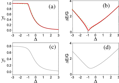
Figure 1: (Color online) Ground state molecular population $y_{0}$ and energy gap $\Delta E$ as functions of $\Delta$. For (a) and (b), $d=0$, the thin black lines represent the semiclassical results, dashed green lines are quantum results for $N=10$, and thick red lines are quantum result for $N=100$. For (c) and (d), $d=0.2$ and only the semiclassical results are shown.

To study the corresponding quantum behavior and its connection with the semiclassical approach, we expand the Hamiltonian (3) using Fock state basis for a given set of $N$ and $D$ and diagonalize the resulting Hamiltonian matrix. Both the quantum and the semiclassical results of ground state molecular population are shown in Fig. 1(a). The quantum calculation always results in a smooth $y_{0}$ curve although it also shows a rapid change from 0 to 1 in a small region near $\Delta=-1$. As expected, the quantum results approach the semiclassical limit as $N$ increases.

Further insights into the properties of the system can be gained by studying the excitations above the ground state. The quantum many-body excited states are obtained in the same manner as above through the diagonalization of the Hamiltonian matrix. We are particularly interested in the “energy gap”, $\Delta E$, defined as the energy difference between the first excited state and the ground state, which is plotted in Fig. 1(b) for several different $N$. The energy gap shows a minimum, which is always finite, at the value of $\Delta$ around which $y_{0}$ rapidly approaches 1. The semiclassical energy gap can be obtained through the following linearization procedure: Substituting $x=x_{0}+\delta x$ and $\varphi=\varphi_{0}+\delta\varphi$ into Eqs. (4) where $(x_{0},\varphi_{0})$ are the steady-state solution and $(\delta x,\delta\varphi)$ represent the small fluctuations away from the steady state, keeping terms up to first order in fluctuations, we have

$$\frac{d}{d\tau}\delta x = -\sqrt{\left(1-x_{0}\right)\left(x_{0}^{2}-d^{2}\right)}\cos\varphi_{0}\delta\varphi,$$

$$\frac{d}{d\tau}\delta\varphi = \left\{-\Lambda-\frac{\left(1-3x_{0}\right)}{\sqrt{\left(1-x_{0}\right)\left(x_{0}^{2}-d^{2}\right)}}\cos\varphi_{0}\right.$$ (6)

$$\left.+\frac{\left(d^{2}+2x_{0}-3x_{0}^{2}\right)^{2}}{4\left[\left(1-x_{0}\right)\left(x_{0}^{2}-d^{2}\right)\right]^{3/2}}\cos\varphi_{0}\right\}\delta x\,,$$

where, in anticipation of later studies, we have not made the assumption of $\Lambda=0$. The oscillation frequency of $\delta x$ and $\delta\varphi$ can be derived straightforwardly as

$$\omega^{2} = \left[\frac{\left(d^{2}+2x_{0}-3x_{0}^{2}\right)^{2}}{4\left(1-x_{0}\right)\left(x_{0}^{2}-d^{2}\right)}+3x_{0}-1\right]\cos^{2}\varphi_{0}$$ (7)

$$-\Lambda\sqrt{\left(1-x_{0}\right)\left(x_{0}^{2}-d^{2}\right)}\cos\varphi_{0}\,.$$

For ground state in the case of $\Lambda=0$, the semiclassical excitation frequency reduces to

$$\omega=\sqrt{\Delta^{2}+3x_{0}-1}\,,$$

which is the semiclassical energy gap. In particular, for $d=0$, we have

$$\omega=\left\{\begin{array}[]{ll}\sqrt{\Delta^{2}-1}\,,&\mathrm{for}\;\Delta\leq-1\\ \left[\Delta^{2}+2-(\sqrt{\Delta^{2}+3}-\Delta)^{2}/3\right]^{1/2}\,,&\mathrm{for}\;\Delta>-1\end{array}\right.$$

which is plotted in Fig. 1(b). The semiclassical energy gap vanishes at the critical point $\Delta=-1$ with a discontinuous jump in its derivative.

Figure 1(a) and (b) clearly show that the quantum result approaches the semiclassical limit as $N\rightarrow\infty$ and hence the much simpler semiclassical theory is reliable for large $N$. Furthermore, there is a critical point at $\Delta=-1$ for $d=0$ in the semiclassical theory which is absent in the quantum calculations with finite $N$, indicating the fact that no true quantum phase transition can occur in a finite system.

We now discuss the case with finite atomic population imbalance, i.e., $d\neq 0$. Although semiclassical solutions to ground state population and excitation can be obtained analytically in the same fashion as in the previous case for $d=0$, the expressions are generally too messy to be instructive. We therefore simply display the results in Fig. 1(c) and (d). Again we find that the semiclassical calculation reproduces the quantum result (not shown in the figure) in the large $N$ limit. One major difference between $d\neq 0$ and $d=0$ is that in the former there is no quantum phase transition even in the semiclassical limit: both the population and the energy gap changes smoothly as $\Delta$ varies, and the energy gap never becomes zero.

From Fig. 1, we can also see that starting from a pure two species atomic condensate, we can coherently create molecular condensate using the method of rapid adiabatic passage, e.g., by tuning $\Delta$ from a large positive value to a large negative value. Near perfect atom-to-molecule conversion footnote is achieved when $\Delta$ is swept adiabatically adiabaticity which is confirmed by our numerical calculations. However, as we demonstrate next, such a smooth conversion of atoms into molecules by a slow sweeping of $\Delta$ cannot be taken for granted when $\Lambda\neq 0$.

III.2 Case 2: $\Lambda\neq 0$

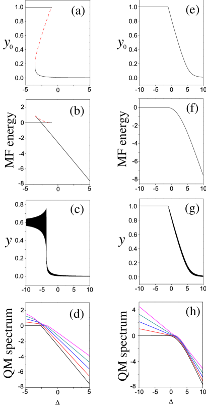
Figure 2: (Color online) Left panel shows an example of dynamical instability with $d=0$ and $\Lambda=-5$. (a) Molecular population in the low lying semiclassical steady states as functions of $\Delta$; the state represented by the red dashed curve is dynamically unstable. (b) Corresponding dimensionless semiclassical mean-field energies as calculated using Eq. (5) ; (c) Molecular population as $\Delta$ is linearly swept; (d) The corresponding quantum many-body energy spectrum for $N=20$, only the lowest five eigenenergies are shown. As the classical Hamiltonian (5) represents energy per pair of atoms, the quantum eigenenergy (in units of $G$) has been rescaled by a factor of $(N/2)^{-1}$. Right panel is the same as the left except for $\Lambda=5$ where there is no dynamical instability.

With a finite $\Lambda$, the algebra becomes much more complicated. We resort to numerical calculations in this case. Consider first the semiclassical situation. The left panel of Fig. 2 illustrates the properties of the system with $d=0$ and $\Lambda=-5$. Fig. 2 (a) and (b) show the molecular population and mean-field energy for the semiclassical steady states. In the region $\Delta\in[-3.56,-1]$, there exist three steady states with similar energies as shown in the figure note . The mean-field energy exhibits a swallowtail loop structure. Similar structures have been observed in condensates moving in optical lattice potentials tail1 and in two-component condensates tail2 under certain conditions, and are associated with dynamical instability.

In our system, by calculating the excitation frequency using Eqs. (6) and (7), we find that one of the three steady states, represented by the red dashed lines in Fig. 2 (a) and (b), possesses imaginary excitation frequency, a signature of dynamical instability. This unstable state links the two stable ones, representing a classical example of bistability which has been intensely studied in the context of nonlinear optics and laser theory note2 . The existence of such a state is the key to the development of atom-molecule switch, the matter wave analog jan of optical bistable switch, for controlling matter waves by matter waves in a coherent and bistable fashion. Under such a bistable situation, no matter how slow we tune $\Delta$, the system will not be able to follow the ground state — when we enter the dynamical unstable region, a discontinuous jump will necessarily occur and the atom-molecule conversion efficiency will suffer. This is confirmed in our numerical simulation as shown in Fig. 2(c) where we linearly sweep $\Delta$ from a large positive to a large negative value starting from a pure two species atomic condensate. In this example, only about 60% of the initial atoms will associate into molecules.

It is instructive to examine the situation from the quantum many-body point of view. Fig. 2(d) shows the five lowest eigenenergies of the quantum Hamiltonian (3) for $N=20$. The quantum mechanical energy spectrum exhibits a net of anticrossings enveloped by a swallowtail loop structure that will morph into the semiclassical energy diagram as shown in Fig. 2(b). Similar semiclassical-quantum correspondence was observed in two-component condensates loop1 ; loop2 and condensates in double-well potentials milburn ; tonel2 .

In comparison, the right panel of Fig. 2 shows a situation without dynamical instability. In this case, rapid adiabatic passage results in a near perfect atom-molecule conversion, and the system follows the ground state closely as $\Delta$ is tuned.

Figure 2 shows that in order to create molecular condensate with high efficiency using the rapid adiabatic passage method, it is of crucial importance to avoid the unstable regimes lps04 . Fig. 3 shows the stability phase diagram in the $\Lambda$-$\Delta$ parameter space. We find that dynamical instability occurs in the region of $\Lambda<-1$ and $\Delta<-1$ and is quite sensitive to atomic population imbalance $d$: With the increase of $d$, the unstable region shrinks. Therefore tuning the population imbalance provides us with a handle to control the dynamical stability of the system.

Figure 3: Stability phase diagram in the $\Lambda$-$\Delta$ parameter space. The black region are dynamically unstable. (a) $d=0$; (b) $d=0.2$.

IV Coherent Atom-Molecule Population Oscillations

Coherent population oscillation has been predicted jm99 ; icn04 ; vya01 ; jkn05 ; stfl06 ; obc04 ; heizen ; sl03 and experimentally measured wieman in systems of homonuclear molecules coupled to atomic condensate. Besides proving the phase coherence between atoms and molecules, a measurement of the oscillation frequency can tell us many properties of the system such as the molecular binding energy, atom-molecule coupling strength, etc. We therefore want to study in this section the population oscillation dynamics in our system starting from a pure atomic cloud, focusing again on the effect of atomic population imbalance.

In a dissipationless system, the total energy is conserved so that the Hamiltonian represents another constant of motion and the semiclassical problem becomes integrable. For an initial state with pure atoms, i.e., $x=1$, the energy constant according to Eq. (5) is $E=-\Delta+\Lambda/2$. By inserting

$$\cos\varphi=\frac{\Delta x-\frac{\Lambda}{2}x^{2}+E}{\sqrt{\left(1-x\right)\left(x^{2}-d^{2}\right)}}\,,$$ (8)

which is obtained from Eq. (5), into Eqs. (4), we can easily find that

$$\left(\frac{dy}{d\tau}\right)^{2} = y\left[1-d^{2}-\left(\Delta^{\prime 2}+2\right)y\right.$$ (9)

$$\left.+\left(1-\Delta^{\prime}\Lambda\right)y^{2}-\Lambda^{2}y^{3}/4\right]\,,$$

where $\Delta^{\prime}=\Delta-\Lambda$ and $y=1-x$ as before.

The solution to Eq. (9) can be expressed in terms of the elliptical functions and strongly depends on the roots of the cubic equations inside the square bracket. A discussion of the solution for the model with homonuclear molecules $\left(d=0\right)$ can be found in Refs. icn04 ; sl03 . Here, in order to gain physical insight into the effect of the population imbalance on the oscillation dynamics, we will focus on the simpler case with $\Lambda=0$. Under this condition, Eq. (9) reduces to

$$\left(\frac{dy}{d\tau}\right)^{2}=y\left[\left(1-y\right)^{2}-d^{2}\right]-\frac{1}{4}\Delta^{2}y^{2}\,,$$

whose solution, when expressed in terms of Jacobi’s elliptic function, has the form

$$y=y_{-}\,\text{sn}^{2}\left(\sqrt{y_{+}}\,\tau/2,\sqrt{y_{-}/y_{+}}\right)\,,$$ (10)

where

$$y_{-} = \frac{1}{2}\frac{1-d^{2}}{1+\frac{\Delta^{2}}{4}+\sqrt{d^{2}-1+\left(1+\frac{\Delta^{2}}{4}\right)^{2}}},$$

$$y_{+} = \frac{1-d^{2}}{4y_{-}}.$$ (11)

Equation (10) describes an undamped oscillation in which $y$ changes from 0 to the peak value $y_{-}$ with a period

$$T=\frac{4F\left(\frac{\pi}{2},\sqrt{y_{-}/y_{+}}\right)}{\sqrt{y_{+}}}\,,$$ (12)

where $F\left(\pi/2,k\right)$ is the complete elliptic integral of the first kind.

Figure 4:  (a) and (b), molecular population oscillation amplitude and period, respectively. The three curves correspond to $d=0$, 0.2 and 0.5 in descending order. (c) Molecular population dynamics for $\Lambda=\Delta=d=0$. Solid line: semiclassical result; dashed and dotted lines: quantum result for $N=100$ and $N=1000$, respectively. (d) On resonance semiclassical oscillation period as a function of $d$.

We plot the amplitude $y_{-}$ and period $T$ of the molecular population oscillation with respect to $\Delta$ for different $d$ in Fig. 4(a) and (b), respectively. The figure is symmetric with respect to $\Delta=0$ so we only present the case with $\Delta\geq 0$. From Eq. (11), we find that for any given $d$, the oscillation reaches a maximum value of

$$y_{-}=1-d\,,$$

at resonance, i.e., $\Delta=0$.

One peculiarity from the semiclassical calculation is that when $d=0$, the oscillation period diverges at $\Delta=0$. In this case we have $y_{+}=y_{-}=1$ and Eq. (10) becomes

$$y=\text{tanh}^{2}\left(\tau/2\right)\,,$$

which shows that atomic (molecular) population decreases (increases) monotonically until all the atoms are converted to molecules. The quantum mechanical calculation, however, does show damped population oscillations under the same condition, as illustrated in Fig. 4(c). The difference between the semiclassical and the quantum results arises because the former does not take atom-molecule entanglement into account. The same behavior will also occur in homonuclear molecule association and has been studied in Ref. vya01 . In heteronuclear molecule association with finite $d$, the period $T$ as given by Eq. (12) never diverges. Using the asymptotic formula for $F(\pi/2,k)$, one can show that, on resonance,

$$T\approx\frac{2}{\sqrt{1+d}}\,\ln\frac{16}{d}\,,$$

for small $d$. The resonant oscillation period as a function of $d$ is shown in Fig. 4(d).

The situation becomes much more complicated in the case of $\Lambda\neq 0$ and in general no simple analytic formula for population oscillation can be found. The general features are nevertheless still preserved: semiclassical result shows undamped oscillation while quantum calculation yields damped oscillation, and the quantum result approaches the semiclassical limit as $N$ increases.

V Conclusion

In conclusion, we have studied coherent association of a two species atomic condensate into heteronuclear molecular condensate using a three-mode model, emphasizing the effect of atomic population imbalance. In particular, the population imbalance, together with detuning and collisional interaction strength, will significantly affect the excitation and stability properties as well as coherent population oscillations of the system. We have also carefully analyzed the differences and connections between the semiclassical and the quantum many-body treatments.

- (1) C. A. Stan, M. W. Zwierlein, C. H. Schunck, S. M. F. Raupach and W. Ketterle, Phys. Rev. Lett. 93, 143001 (2004).
- (2) S. Inouye, J. Goldwin, M. L. Olsen, C. Ticknor, J. L. Bohn and D. S. Jin, Phys. Rev. Lett. 93, 183201 (2004).
- (3) C. Ospelkaus, S. Ospelkaus, L. Humbert, P. Ernst, K. Sengstock and K. Bongs, Phys. Rev. Lett. 97, 120402 (2006); S. Ospelkaus, C. Ospelkaus, L. Humbert, K. Sengstock, and K. Bongs, Phys. Rev. Lett. 97, 120403 (2006).
- (4) A. J. Kerman, J. M. Sage, S. Sainis, T. Bergeman and D. Demille, Phys. Rev. Lett. 92, 153001 (2004).
- (5) C. Haimberger, J. Kleinert, M. Bhattacharya and N. P. Bigelow, Phys. Rev. A 70, 021402(R) (2004).
- (6) D. Wang, J. Qi, M. F. Stone, O. Nikolayeva, H. Wang, B. Hattaway, S. D. Gensemer, P. L. Gould, E. E. Eyler, and W. C. Stwalley, Phys. Rev. Lett. 93, 243005 (2004).
- (7) E. A. Donley, N. R. Claussen, S. T. Thompson, and C. E. Wieman, Nature 417, 529 (2002).
- (8) H. Y. Ling, H. Pu and B. Seaman, Phys. Rev. Lett. 93, 250403 (2004); H. Y. Ling, P. Maenner, and H. Pu, Phys. Rev. A 72, 013608 (2005).
- (9) S. J. J. M. F. Kokkelmans, H. M. J. Vissers and B. J. Verhaar, Phys. Rev. A 63, 031601 (2001).
- (10) M. Mackie, R. Kowalski and J. Javananinen, Phys. Rev. Lett. 84, 3803 (2000).
- (11) C. P. Search and P. Meystre, Phys. Rev. Lett. 93, 140405 (2004).
- (12) A. Nunnenkamp, D. Meiser and P. Meystre, New J. of Phys. 8, 88 (2006).
- (13) M. Duncan, A. Foerster, J. Links, E. Mattei, N. Oelkers, A. P. Tonel, Nucl. Phys. B 767, 227 (2007).
- (14) Y. Wu and R. Côté, Phys. Rev. A 65, 053603 (2002).
- (15) J. Javananinen and M. Mackie, Phys. Rev. A 59, 3186(R) (1999).
- (16) A. Ishkhanyan, G. P. Chernikov and H. Nakamura, Phys. Rev. A 70, 053611 (2004).
- (17) A. Vardi, V. A. Yurovsky and J. R. Anglin, Phys. Rev. A 64, 063611 (2001).
- (18) G.-R. Jin, C. K. Kim and K. Nahm, Phys. Rev. A 72, 045602 (2005).
- (19) G. Santos, A. Tonel, A. Foerster and J. Links, Phys. Rev. A 73, 023609 (2006).
- (20) B. Seaman and Hong Y. Ling, Opt. Comm. 226, 267 (2003).
- (21) D. J. Heinzen, R. Wynar, P. D. Drummond, and K. V. Kheruntsyan, Phys. Rev. Lett. 84, 5029 (2000).
- (22) M. K. Olsen, A. S. Bradley and S. B. Cavalcanti, Phys. Rev. A 70, 033611 (2004).
- (23) P. D. Drummond, K. V. Kheruntsyan and H. He, Phys. Rev. Lett. 81, 3055 (1998).
- (24) H. Uys, T. Miyakawa, D. Meiser and P. Meystre, Phys. Rev. A 72, 053616 (2005).
- (25) M. W. Jack and H. Pu, Phys. Rev. A 72, 063625 (2005).
- (26) T. Miyakawa and P. Meystre, Phys. Rev. A 74, 043615 (2006).
- (27) C. M. Savage, P. E. Schwenn and K. V. Kheruntsyan, Phys. Rev. A 74, 033620 (2006); K. V. Kheruntsyan, Phys. Rev. Lett. 96, 110401 (2006).
- (28) B. Damski, L. Santos, E. Tiemann, M. Lewenstein, S. Kotochigova, P. Julienne, and P. Zoller, Phys. Rev. Lett. 90, 110401 (2003).
- (29) D. DeMille, Phys. Rev. Lett. 88, 067901 (2002).
- (30) A. Micheli, G. K. Brennen, and P. Zoller, Nature Phys. 2, 341 (2006).
- (31) M. G. Kozlov, and L. N. Labzowsky, J. Phys. B 28, 1933 (1995).
- (32) M. W. Zwierlein, A. Schirotzek, C. H. Schunch, and W. Ketterle, Science 311, 492 (2006).
- (33) G. B. Patridge, W. Li, R. I. Kamar, Y. A. Liao, and R. G. Hulet, Science 311, 503 (2006); G. B. Patridge, W. Li, Y. A. Liao, R. G. Hulet, M. Haque, and H. T. C. Stoof, Phys. Rev. Lett. 97, 190407 (2006).
- (34) See, for example, J. R. Anglin, and A. Vardi, Phys. Rev. A 64, 013605 (2001) and references therein.
- (35) C. K. Law, H. Pu and N. P. Bigelow, Phys. Rev. Lett. 81, 5257 (1998).
- (36) G. Drobný, I. Jex and V. Bužek, Phys. Rev. A 48, 569 (1993).
- (37) K.-P. Marzlin and J. Audretsch, Phys. Rev. A 57, 1333 (1998).
- (38) One can measure the atom-molecule conversion efficiency by the final molecular population, . In the presence of atomic population imbalance, the maximum possible value for is . Therefore one can define as the conversion efficiency.
- (39) H. Pu, P. Maenner, W. Zhang, and H. Y. Ling, Phys. Rev. Lett. 98, 050406 (2007).
- (40) Except for the steady state with whose relative phase is undefined, for the other two steady states. There also exsit one or more steady states with . These states have higher energies and are not shown in the figure.
- (41) B. Wu, R. B. Diener, and Q. Niu, Phys. Rev. A 65, 025601 (2002); D. Diakonov, L. M. Jensen, C. J. Pethick, and H. Smith, Phys. Rev. A 66, 013604 (2002).
- (42) B. Wu, and Q. Niu, Phys. Rev. A 61, 023402 (2000).
- (43) See for example, H. Gibbs, Optical Bistability (Academic Press, 1985).
- (44) J. Heurich, H. Pu, M. G. Moore, and P. Meystre, Phys. Rev. A 63, 033605 (2001).
- (45) Z. P. Karkuszewski, K. Sacha, and A. Smerzi, Eur. Phys. J. D 21, 251 (2002).
- (46) B. Wu, and J. Liu, Phys. Rev. Lett. 96, 020405 (2006).
- (47) G. J. Milburn, J. Corney, E. M. Wright and D. F. Walls, Phys. Rev. A 55, 4318 (1997).
- (48) A. P. Tonel, J. Links and A. Foerster, J. Phys. A 38, 6879 (2005).