Monogamy of Bell correlations and Tsirelson’s bound

Abstract

We consider three parties, A, B, and C, each performing one of two local measurements on a shared quantum state of arbitrary dimension. We characterize the trade-off between the nonlocality of the Bell correlations observed by AB and of those observed by AC. This generalizes Tsirelson’s bound on the quantum value of the CHSH inequality, the latter being recovered when C is completely uncorrelated with AB. We also discuss the trade-off between Bell violations and local expectation values of observables that anticommute with the ones used in the Bell test.

The existence of Bell inequalities Bell (1964); Clauser et al. (1969) and their observed violation in experiments has had a very deep impact on the way we look at quantum mechanics. On the one hand, it has led to a study of the precise meaning of nonlocality and opened up the field of entanglement theory. On the other, it has led to the observation that Bell violations can be exploited in the design of cryptographic protocols Ekert (1991). In that case, an eavesdropper (C) tries to gain access to some quantum correlations shared by Alice (A) and Bob (B). If the Bell correlations between A and B are strong, it can happen that C’s outcomes will be almost uncorrelated with them, and A and B will be able to execute a purification protocol so as to create private randomness. In the present paper, we will make a precise quantitative statement about the following monogamy property: Suppose A and B violate a Bell inequality by a certain amount. How does that bound the possible Bell correlations between A and C? This is also interesting from the point of view of entanglement theory, as it provides monogamy relations independent of the size of the local Hilbert spaces. For the Clauser-Horne-Shimony-Holt (CHSH) inequality, the region of accessible Bell correlations between AB and AC turns out to be very simple (see Figure 1).

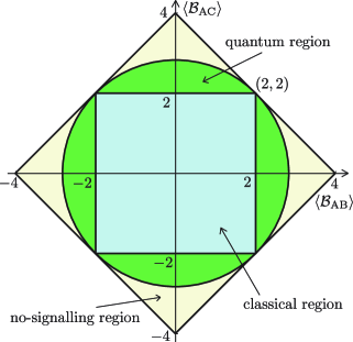
Figure 1: Accessible values of $\langle\mathcal{B}_{\text{AB}}\rangle$ and $\langle\mathcal{B}_{\text{AC}}\rangle$ for classical theories (interior of square), quantum theory (interior of circle), and no-signalling theories (interior of diamond). Note that both quantum and no-signalling theories obey monogamy constraints; classical local hidden variable theories do not.

In the setting where two parties, A and B, share a quantum state $\rho$, and each has the choice of two local measurements, there is just one relevant Bell inequality, the CHSH inequality Clauser et al. (1969). Define the CHSH operator

$${\cal B}_{\text{AB}}={A}_{1}\otimes\left({B}_{1}+{B}_{2}\right)+{A}_{2}\otimes\left({B}_{1}-{B}_{2}\right),$$ (1)

where ${A}_{1}$ and ${A}_{2}$ (${B}_{1}$ and ${B}_{2}$) are A’s (B’s) observables and are Hermitian operators with spectrum in $[-1,+1]$. For particular measurements and a particular state $\rho$, the quantum value of the CHSH inequality is defined as $\langle\mathcal{B}_{\text{AB}}\rangle=\operatorname{tr}\left({\cal B}_{\text{AB}}\rho\right)$. All correlations described by local hidden variable (LHV) models satisfy the CHSH inequality, $\left|\langle\mathcal{B}_{\text{AB}}\rangle_{\text{LHV}}\right|\leq 2$, but in the case of entangled quantum systems, this bound can be violated. For example, on the singlet state of two qubits there exist operators $A_{i},B_{i}$ such that $\langle\mathcal{B}_{\text{AB}}\rangle=\langle\psi^{-}|{\cal B}_{\text{AB}}|\psi^{-}\rangle=2\sqrt{2}$.

We do not yet know how to calculate a bound on the maximum quantum value of an arbitrary Bell inequality, but a number of ad hoc techniques have been developed Cirel’son (1980); Tsirelson (1987); Toner (2006); Navascues et al. . In the case of the CHSH inequality, Tsirelson has proved that $\left|\operatorname{tr}\left({\cal B}_{\text{AB}}\rho\right)\right|\leq 2\sqrt{2}$ for all observables ${A}_{1}$, ${A}_{2}$, ${B}_{1}$, ${B}_{2}$, and all states $\rho$ Cirel’son (1980). This Tsirelson bound can itself be violated if we consider more general hypothetical no-signalling theories: a nonlocal box violates the CHSH inequality maximally, $\langle\mathcal{B}_{\text{AB}}\rangle_{\text{NL}}=4$ Popescu and Rohrlich (1994). Tsirelson’s bound is a simple mathematical consequence of the axioms of quantum theory, but is there some deeper reason why a violation greater than $2\sqrt{2}$ is unphysical? For example, a violation greater than $\sqrt{32/3}\approx 3.27$ would imply that any communication complexity problem can be solved using a constant amount of communication van Dam (2005). As will be clear from the following results, the bound $2\sqrt{2}$ is very natural if one considers the possible Bell violations in a three-party setup.

We establish the following monogamy trade-off:

Theorem 1.

Suppose that three parties, A, B, and C, share a quantum state (of arbitrary dimension) and each chooses to measure one of two observables. Then

$$\langle\mathcal{B}_{\text{AB}}\rangle^{2}+\langle\mathcal{B}_{\text{AC}}\rangle^{2}\leq 8.$$ (2)

Here, $\mathcal{B}_{\text{AC}}$ is defined as in Eq. (1), but with B’s observables replaced by C’s. Note that we obtain Tsirelson’s bound, $\langle\mathcal{B}_{\text{AB}}\rangle^{2}\leq 8$, as a simple corollary. Note also that A’s measurements are the same in $\langle\mathcal{B}_{\text{AB}}\rangle$ and $\langle\mathcal{B}_{\text{AC}}\rangle$: otherwise we could have $\langle\mathcal{B}_{\text{AB}}\rangle=\langle\mathcal{B}_{\text{AC}}\rangle=2\sqrt{2}$ and there would be no trade-off. Theorem 1 is analogous to the Coffman-Kundu-Wootters theorem that describes the trade-off between how entangled A is with B, and how entangled A is with C Coffman et al. (2000). Eq. (2) is the best possible bound: there are states and measurements achieving any values of $\langle\mathcal{B}_{\text{AB}}\rangle$ and $\langle\mathcal{B}_{\text{AC}}\rangle$ that satisfy it. Previously the best bound known was $\left|\langle\mathcal{B}_{\text{AB}}\rangle\right|+\left|\langle\mathcal{B}_{\text{AC}}\rangle\right|\leq 4$, which is tight for correlations that arise from no-signalling theories Toner (2006); Masanes et al. (2006). We illustrate the monogamy trade-offs for various theories in Figure 1.

We prove Theorem 1 in two parts. We first show that is sufficient to restrict to states with support on a qubit at each site. We can then relax the requirement that A’s measurements be the same in $\langle\mathcal{B}_{\text{AB}}\rangle$ and $\langle\mathcal{B}_{\text{AC}}\rangle$, maximizing over the measurements in $\langle\mathcal{B}_{\text{AB}}\rangle$ and $\langle\mathcal{B}_{\text{AC}}\rangle$ separately, but keeping the state fixed. Our proof suggests a connection between anticommutation and Bell inequality violation, which we then explore more deeply.

Dimensional reduction.—We start by establishing a bound on the dimension of the quantum state required to maximally violate certain Bell inequalities. A similar result was proved by Masanes Masanes (2005). The main ingredient—a canonical decomposition for a pair of subspaces of $\mathbb{C}^{n}$—is described in more detail in, e.g., Ref. Bhatia (1996).

Lemma 2.

Consider any Bell inequality in the setting where $m$ parties each choose from two two-outcome measurements. Then the maximum quantum value of the Bell inequality is achieved by a state that has support on a qubit at each site. Furthermore, we can assume this state has real coefficients and that the observables are real and traceless.

Proof.

For $i\in\{1,2\}$, assume party $k$ has observables ${M}_{k,i}$, acting on a Hilbert space ${\cal H}_{k}$. By extending the local Hilbert spaces ${\cal H}_{k}$, we can assume for all $k$ and for all $i=1,2$ that (i) ${\cal H}_{k}=\mathbb{C}^{2d}$ for some fixed $d$, (ii) ${M}_{k,i}$ has eigenvalues $\pm 1$, and (iii) $\operatorname{tr}{M}_{k,i}=0$. The first condition states that all local spaces have the same dimension $2d$, the latter two that each observable corresponds to a projective measurement onto a $d$-dimensional subspace and its complement. We also define ${M}_{k,0}=\leavevmode\hbox{\small 1\normalsize\kern-3.30002pt1}_{2d}$, the identity operator on ${\cal H}_{k}$. We can write a generic Bell operator in the setting stated in the lemma as

$${\cal B}=\sum_{i_{1}=0}^{2}\sum_{i_{2}=0}^{2}\cdots\sum_{i_{m}=0}^{2}c_{i_{1}i_{2}\cdots i_{m}}\bigotimes_{k=1}^{m}{M}_{k,i_{k}},$$ (3)

where the coefficients $c_{i_{1}i_{2}\cdots i_{m}}$ are arbitrary real numbers. Our goal is find the quantum value of this Bell operator, which is maximum of $B\equiv\langle\psi|\cal B|\psi\rangle$ over states $|\psi\rangle$ and measurements ${M}_{k,i}$.

We now choose a local basis for each ${\cal H}_{k}$ such that party $k$’s observables have a simple form. We start by taking ${M}_{k,1}=\left[\vbox{\hbox{\kern-1.15198pt\raise 0.0pt\hbox{\kern 28.16283pt}\kern 0.0pt\vbox{}\kern-1.15198pt}}\right]$. This leaves us the freedom to specify the basis within the two $d\times d$ blocks on which ${M}_{k,1}$ is constant. Let ${M}_{k,2}=2{P}{P}^{\dagger}-\leavevmode\hbox{\small 1\normalsize\kern-3.30002pt1}_{2d}$ (we suppress the dependence on $k$), where ${P}$ is a $2d\times d$ matrix with orthonormal columns, which span the $+1$–eigenspace of ${M}_{k,2}$). Write ${P}=\left[\vbox{\hbox{\kern-1.15198pt\raise 0.0pt\hbox{\kern 10.60904pt}\kern 0.0pt\vbox{}\kern-1.15198pt}}\right]$, where ${P}_{1}$ and ${P}_{2}$ are $d\times d$ matrices. The rows of $P$ are orthonormal, which implies ${P}^{\dagger}{P}={P}_{1}^{\dagger}{P}_{1}+{P}_{2}^{\dagger}{P}_{2}=\leavevmode\hbox{\small 1\normalsize\kern-3.30002pt1}_{d}$, so ${P}_{1}^{\dagger}{P}_{1}$ and ${P}_{2}^{\dagger}{P}_{2}$ are simultaneously diagonalizable. This means there is a singular value decomposition of the form ${P}_{1}={U}_{1}^{\dagger}{D}_{1}{V}$, ${P}_{2}={U}_{2}^{\dagger}{D}_{2}{V}$, where ${U}_{1}$, ${U}_{2}$ and $V$ are $d\times d$ unitary matrices and ${D}_{1}$ and ${D}_{2}=\sqrt{\leavevmode\hbox{\small 1\normalsize\kern-3.30002pt1}_{d}-{D}_{1}^{2}}$ are nonnegative (real) diagonal matrices. Changing basis according to the unitary ${U}_{1}\oplus{U}_{2}$, which leaves ${M}_{k,1}$ invariant, it follows that ${M}_{k,2}=\left[\vbox{\hbox{\kern-1.15198pt\raise 0.0pt\hbox{\kern 64.21008pt}\kern 0.0pt\vbox{}\kern-1.15198pt}}\right]$, where each of the $d\times d$ blocks is diagonal. We relabel our basis vectors so that ${M}_{k,1}=\bigoplus_{j=1}^{d}{Z}$, $M_{k,2}=\bigoplus_{j=1}^{d}\left(\cos\theta_{j}{Z}+\sin\theta_{j}{X}\right)$, where $2{D}_{1}^{2}-\leavevmode\hbox{\small 1\normalsize\kern-3.30002pt1}_{d}=\mathrm{diag}(\cos\theta_{1},\cos\theta_{2},\ldots,\cos\theta_{d})$ and $X$ and $Z$ are the usual Pauli operators. Hence our operators are real and preserve a $\oplus_{j=1}^{d}\mathbb{C}^{2}$ subspace of ${\cal H}_{k}$. They are traceless on each $\mathbb{C}^{2}$ space.

We wish to maximize $B=\langle\psi|\cal B|\psi\rangle$ over the state $|\psi\rangle$ and the measurements ${M}_{k,i}$. Fix $k$, and let $\rho_{k,j}$ be the reduced density matrix obtained by projecting $|\psi\rangle$ onto the $j$’th $\mathbb{C}^{2}$ factor of the $\oplus_{j=1}^{d}\mathbb{C}^{2}$ subspace induced by $M_{k,1}$ and $M_{k,2}$ at site $k$. Then $B=\sum_{j=1}^{d}\operatorname{tr}{\cal B}\rho_{k,j}$ is a convex sum over the $\mathbb{C}^{2}$ factors, whereupon it follows that the maximum is achieved by a state with support on a qubit at site $k$. Since this argument works for all $k$, the maximum of $B$ is achieved by a state that has support on a qubit on each site.

Finally, write $|\psi\rangle=|\psi_{1}\rangle+i|\psi_{2}\rangle$, where $|\psi_{1}\rangle$ and $|\psi_{2}\rangle$ are real. Then $\langle\psi|{\cal B}|\psi\rangle=\langle\psi_{1}|{\cal B}|\psi_{1}\rangle+\langle\psi_{2}|{\cal B}|\psi_{2}\rangle$ since $\cal B$ is real, which is the same expression we would obtain if the state were a real mixture of $|\psi_{1}\rangle$ and $|\psi_{2}\rangle$. Hence the maximum of $B$ is achieved by a state with real coefficients. ∎

Monogamy trade-off relation.—The region $\cal R$ of allowed values of $\left(\langle\mathcal{B}_{\text{AB}}\rangle,\langle\mathcal{B}_{\text{AC}}\rangle\right)$ is convex and can therefore be described by an (infinite) family of half-space inequalities,

$$c_{\text{AB}}\langle\mathcal{B}_{\text{AB}}\rangle+c_{\text{AC}}\langle\mathcal{B}_{\text{AC}}\rangle\leq d,$$ (4)

with $c_{\text{AB}},c_{\text{AC}},d\in\mathbb{R}$. The left-hand side of Eq. (4) is a Bell operator, as defined in Eq. (3), which means we can apply Lemma 2 to conclude that extreme points of $\cal R$ are achieved by real states on three qubits, with measurements of the form ${M}=\cos\theta{Z}+\sin\theta{X}$. Theorem 1 will emerge as a corollary of:

Lemma 3.

Let $|\psi\rangle$ be a pure state in $\mathbb{C}^{2}\otimes\mathbb{C}^{2}\otimes\mathbb{C}^{2}$ with real coefficients. Then the maximum of $\left\langle\mathcal{B}_{\mathrm{AB}}\right\rangle$ over real traceless observables ${A}_{1},{A}_{2},{B}_{1},{B}_{2}$ is

$$2\sqrt{1+\left\langle{{Y}}_{\mathrm{A}}{{Y}}_{\mathrm{B}}\right\rangle^{2}-\left\langle{{Y}}_{\mathrm{A}}{{Y}}_{\mathrm{C}}\right\rangle^{2}-\left\langle{{Y}}_{\mathrm{B}}{{Y}}_{\mathrm{C}}\right\rangle^{2}},$$ (5)

where $Y$ is the usual Pauli operator, $\left\langle{{Y}}_{\mathrm{A}}{{Y}}_{\mathrm{B}}\right\rangle=\operatorname{tr}\left(Y_{A}\otimes Y_{B}\otimes\leavevmode\hbox{\small 1\normalsize\kern-3.30002pt1}\,\rho\right)$, and so on. Cyclic permutations of Eq. (5) hold for $\langle\mathcal{B}_{\mathrm{AC}}\rangle$ and $\langle\mathcal{B}_{\mathrm{BC}}\rangle$.

Proof.

We consider $\rho_{AB}=\operatorname{tr}_{C}|\psi\rangle\langle\psi|$, which is a real state on $\mathbb{C}^{2}\otimes\mathbb{C}^{2}$. Horodecki and family have calculated the maximum quantum value of the CHSH operator for a state on $\mathbb{C}^{2}\otimes\mathbb{C}^{2}$ Horodecki et al. (1996). Their analysis simplifies in our case because the state and measurements are real. Define

$$T_{\text{AB}}=\left[\begin{matrix}\langle X_{A}X_{B}\rangle&\langle X_{A}Z_{B}\rangle\\ \langle Z_{A}X_{B}\rangle&\langle Z_{A}Z_{B}\rangle\end{matrix}\right].$$ (6)

For $i=1,2$, write ${A}_{i}=\hat{a}_{i}\cdot\vec{\sigma}_{r}$, ${B}_{i}={\hat{b}}_{i}\cdot\vec{\sigma}_{r}$, where $\hat{a}_{i}$ and $\hat{b}_{i}$ are two-dimensional unit vectors and $\vec{\sigma}_{r}=({X},{Z})$. Define

$$\hat{b}_{1}+\hat{b}_{2}=2\cos\theta\hat{d}_{1},\ \ \hat{b}_{1}-\hat{b}_{2}=2\sin\theta\hat{d}_{2},$$ (7)

where $\theta\in[0,\pi/2]$ and $\hat{d}_{1}$ and $\hat{d}_{1}$ are orthogonal unit vectors. Then

$$\frac{1}{2}\max_{{A}_{i},{B}_{j}}\left\langle\mathcal{B}_{\mathrm{AB}}\right\rangle = \max_{\hat{d}_{i},\theta,\hat{a}_{i}}\cos\theta\hat{a}_{1}^{t}T_{\text{AB}}\hat{d}_{1}+\sin\theta\hat{a}_{2}^{t}T_{\text{AB}}\hat{d}_{2}$$ (8)

$$= \max_{\hat{d}_{i},\theta}\cos\theta\left\|T_{\text{AB}}\hat{d}_{1}\right\|+\sin\theta\left\|T_{\text{AB}}\hat{d}_{2}\right\|$$

$$= \max_{\hat{d}_{i}}\sqrt{\left\|T_{\text{AB}}\hat{d}_{1}\right\|^{2}+\left\|T_{\text{AB}}\hat{d}_{2}\right\|^{2}}$$

$$= \sqrt{\operatorname{tr}\left({T_{\text{AB}}}{T_{\text{AB}}}^{t}\right)}.$$ (9)

This is just the Frobenius norm of $T_{\text{AB}}$ and it is straightforward to check that, for pure states on $\mathbb{C}^{2}\otimes\mathbb{C}^{2}\otimes\mathbb{C}^{2}$ with real coefficients, it is equal to half of Eq. (5).∎

Lemma 4.

For a pure state $|\psi\rangle$ with real coefficients in $\mathbb{C}^{2}\otimes\mathbb{C}^{2}\otimes\mathbb{C}^{2}$,

$$\max_{{A}_{i},{B}_{j},{C}_{k}}\left\langle\mathcal{B}_{\mathrm{AB}}\right\rangle^{2}+\left\langle\mathcal{B}_{\mathrm{AC}}\right\rangle^{2}=8\left(1-\left\langle{{Y}}_{\mathrm{B}}{{Y}}_{\mathrm{C}}\right\rangle^{2}\right).$$ (10)

Proof.

Lemma 3, applied to $\langle\mathcal{B}_{\text{AB}}\rangle$ and $\langle\mathcal{B}_{\text{AC}}\rangle$ separately, immediately implies:

$$\max_{{A}_{i},{B}_{j},{C}_{k}}\left\langle\mathcal{B}_{\mathrm{AB}}\right\rangle^{2}+\left\langle\mathcal{B}_{\mathrm{AC}}\right\rangle^{2} \leq \max_{{A}_{i},{B}_{j}}\left\langle\mathcal{B}_{\mathrm{AB}}\right\rangle^{2}+\max_{{A}_{i},{C}_{k}}\left\langle\mathcal{B}_{\mathrm{AC}}\right\rangle^{2}$$ (11)

$$= 8\left(1-\left\langle{{Y}}_{\mathrm{B}}{{Y}}_{\mathrm{C}}\right\rangle^{2}\right).$$

The reason we do not have equality is that the measurements $A_{i}$ achieving the maximum in $\langle\mathcal{B}_{\text{AB}}\rangle$ and $\langle\mathcal{B}_{\text{AC}}\rangle$ may be different. We have to show they can be chosen to be the same. Define $T_{\text{AC}}$ in analogy with Eq. (6) and write the vectors corresponding to C’s measurements as

$$\hat{c}_{1}+\hat{c}_{2}=2\cos\theta\hat{e}_{1},\ \ \hat{c}_{1}-\hat{c}_{2}=2\sin\theta\hat{e}_{2},$$ (12)

in analogy with Eq. (7) for B’s observables. One can check that $\left[T_{\text{AB}}T_{\text{AB}}^{t},T_{\text{AC}}T_{\text{AC}}^{t}\right]=0$ for all pure states $|\psi\rangle$ with real coefficients. Hence there are orthonormal vectors $a^{\prime}_{1}$ and $a^{\prime}_{2}$ that are simultaneous eigenvectors of $T_{\text{AB}}T_{\text{AB}}^{t}$ and $T_{\text{AC}}T_{\text{AC}}^{t}$. Next, note that the term being maximized in Eq. (8), $\|T_{\text{AB}}\hat{d}_{1}\|^{2}+\|T_{\text{AB}}\hat{d}_{2}\|^{2}$, is actually independent of the $\hat{d}_{i}$ (recall that $\hat{d}_{1}\cdot\hat{d}_{2}=0$), so we are free to choose the $\hat{d}_{i}$ as we please. Take $\hat{d}_{i}=T^{t}_{\text{AB}}\hat{a}_{i}^{\prime}$ for $i=1,2$ and, similarly, take $\hat{e}_{i}=T^{t}_{\text{AC}}\hat{a}_{i}^{\prime}$. Alice’s measurement vector $\hat{a}_{i}$ in the AB maximization of the previous lemma was taken to be the unit vector along $T_{\text{AB}}\hat{d}_{i}$, but this is $T_{\text{AB}}T^{t}_{\text{AB}}\hat{a}^{\prime}_{i}\propto\hat{a}^{\prime}_{i}$ so $\hat{a}_{i}=\hat{a}^{\prime}_{i}$. The same will hold in the AC maximization. Hence we can choose A’s measurement vectors to be the same in both cases, and we have equality in Eq. (10). ∎

Combining Lemmas 2 and 4, we obtain Theorem 1.

The monogamy trade-off is tight.—Lemma 4 also implies that any $\langle\mathcal{B}_{\text{AB}}\rangle$ and $\langle\mathcal{B}_{\text{AC}}\rangle$ compatible with Eq. (10) are achievable. In particular, the state

$$|\psi\rangle=c_{-}\left(|010\rangle+|011\rangle\right)+c_{+}\left(|100\rangle+|101\rangle\right),$$ (13)

where

$$c_{\pm}=\frac{1}{2}\,\sqrt{1\pm\sqrt{2}\sin t},$$ (14)

and $0\leq t\leq\pi/4$, gives $\langle\mathcal{B}_{\text{AB}}\rangle=2\sqrt{2}\,\cos t$, $\langle\mathcal{B}_{\text{AC}}\rangle=2\sqrt{2}\,\sin t$.

Extensions.—In the case of the CHSH inequality we can, in principle, obtain monogamy trade-offs when there are more than three parties via Lemma 2, which converts the problem into a finite optimization problem. In the three-party setting, if we are interested in $\langle\mathcal{B}_{\text{BC}}\rangle$ as well as $\langle\mathcal{B}_{\text{AB}}\rangle$ and $\langle\mathcal{B}_{\text{AC}}\rangle$ then we can obtain the trade-off surface numerically. The technique of Lemma 4—to allow A’s measurements to be different in $\langle\mathcal{B}_{\text{AB}}\rangle$ and $\langle\mathcal{B}_{\text{AC}}\rangle$ and then show that they could be the same anyway—does not work. It predicts that the trade-off surface be the intersection of the three cylinders, $\langle\mathcal{B}_{\text{AB}}\rangle^{2}+\langle\mathcal{B}_{\text{AC}}\rangle^{2}\leq 8$, $\langle\mathcal{B}_{\text{AB}}\rangle^{2}+\langle\mathcal{B}_{\text{BC}}\rangle^{2}\leq 8$, and $\langle\mathcal{B}_{\text{AC}}\rangle^{2}+\langle\mathcal{B}_{\text{BC}}\rangle^{2}\leq 8$, but one can show, for example by using the multipartite generalization of Navascues, Pironio and Acín’s semidefinite programming bounds Navascues et al. , that there are points on this surface that are not achievable. It would be interesting to extend the semidefinite programming technique to obtain monogamy inequalities for other Bell inequalities.

Bell inequality violation and anticommutation.—The precise form of Eq. (10) suggests a general connection between the trade-off of Bell inequality violation and the expectation values of anticommuting observables; indeed, the operator $Y_{B}Y_{C}$ anticommutes with all observables $B_{j},C_{k}$ measured in the Bell test. We now give a more general result, restricting for simplicity to the two party case.

Theorem 5.

Let ${\cal B}=\sum_{i,j=1}^{n}p_{ij}A_{i}\otimes B_{j}$ be a 2-party 2-outcome correlation Bell operator such that $\operatorname{tr}\rho{\cal B}\leq{\cal Q}$ for all shared states $\rho$ and all observables $A_{i}$, $B_{j}$ (with spectrum in $[-1,+1]$). Let $W$ be any observable (with spectrum in $[-1,+1]$) on Bob’s Hilbert space that anticommutes with $B_{j}$ for all $j$. Then

$$\operatorname{tr}\rho{\cal B}\leq{\cal Q}\sqrt{1-\left(\operatorname{tr}\rho W\right)^{2}}.$$ (15)

Proof.

We start by noting that it is sufficient to restrict to the case where $\rho$ is pure, i.e., $\rho=|\psi\rangle\langle\psi|$. The general case then follows by applying Jensen’s inequality to the concave function $f(x)=\sqrt{1-x^{2}}$.

If $|w\rangle$ is an eigenvector of $W$ with eigenvalue $w$, $B_{j}|w\rangle$ is either 0 or an eigenvector of $W$ with eigenvalue $-w$, since $B_{j}$ and $W$ anticommute. This means that there is a decomposition ${\cal H}_{B}={\cal W}_{0}\oplus{\cal W}_{1}\oplus{\cal W}_{2}$, where $W$ annihilates vectors in ${\cal W}_{0}$, every $B_{j}$ annihilates vectors in ${\cal W}_{1}$, and ${\cal W}_{2}$ is spanned by eigenvectors of $W$ with nonzero eigenvalues, which occur in positive/negative pairs.

Denote the distinct positive eigenvalues associated with eigenvectors of $W$ in ${\cal W}_{2}$ as $0<w_{2}<w_{3}<\cdots<w_{m}\leq 1$ and let $V_{i}^{\pm}$ be the subspace in ${\cal W}_{2}$ corresponding to eigenvalue $\pm w_{i}$. Decompose $|\psi\rangle$ as $|\psi\rangle=\sum_{i=0}^{m}\sqrt{p_{i}}|\psi_{i}\rangle$, where $\sum_{i}p_{i}=1$, $|\psi_{0}\rangle\in{\cal W}_{0}$, $|\psi_{1}\rangle\in{\cal W}_{1}$, $\langle\psi_{0}|\psi_{0}\rangle=\langle\psi_{1}|\psi_{1}\rangle=1$, and for $i\geq 2$, $|\psi_{i}\rangle=\left(\cos\theta_{i}|w_{i}^{+}\rangle+\sin\theta_{i}|w_{i}^{-}\rangle\right)$, $|w_{i}^{\pm}\rangle\in V_{i}^{\pm}$, and $\langle w_{i}^{\pm}|w_{i}^{\pm}\rangle=1$. Then ${\cal B}|w_{i}^{\pm}\rangle\in V_{i}^{\mp}$ for $i\geq 2$. It follows that

$$\langle\psi|{\cal B}|\psi\rangle = p_{0}\langle\psi_{0}|{\cal B}|\psi_{0}\rangle+\sum_{i=2}^{m}p_{i}\mathrm{Re}\left(\langle w_{i}^{+}|{\cal B}|w_{i}^{-}\rangle\right)\sin 2\theta_{i},$$

$$\langle\psi|W|\psi\rangle = p_{1}\langle\psi_{1}|W|\psi_{1}\rangle+\sum_{i=2}^{m}p_{i}w_{i}^{2}\cos 2\theta_{i}.$$ (16)

But these are the same expressions we would obtain with the mixed state $\rho=\sum_{i}p_{i}|\psi_{i}\rangle\langle\psi_{i}|$. It therefore follows from our initial remark that it is sufficient to prove the claim for each state $|\psi_{i}\rangle$. For $i=0,1$, the result is trivial. Fix $i\geq 2$, set $\chi=\mathrm{Re}\left(\langle w_{i}^{+}|{\cal B}|w_{i}^{-}\rangle\right)$ and let $x\in\{\pm 1\}$ be the sign of $\chi$. Set $|\phi\rangle=\frac{1}{\sqrt{2}}|w_{i}^{-}\rangle+x\frac{1}{\sqrt{2}}|w_{i}^{+}\rangle$. Then $\langle\phi|{\cal B}|\phi\rangle=\chi<Q$ by assumption, while

$$\langle\psi_{i}|{\cal B}|\psi_{i}\rangle \leq \chi\sin 2\theta_{i}$$ (17)

$$\leq \chi\sqrt{1-\langle\psi_{i}|W|\psi_{i}\rangle^{2}}$$ (18)

$$\leq Q\sqrt{1-\langle\psi_{i}|W|\psi_{i}\rangle^{2}}.$$ (19)

This completes the proof. ∎

We now apply Theorem 5 to the CHSH inequality. If $B_{1}$ and $B_{2}$ are observables with $\pm 1$ eigenvalues, then they both anticommute with their commutator $i[B_{1},B_{2}]/2$ (the factor of $i/2$ makes this an observable). Applying Theorem 5 to both Alice and Bob’s observables, it follows that

$$\langle\mathcal{B}_{\text{AB}}\rangle \leq 2\sqrt{2-\left|\langle[B_{1},B_{2}]\rangle\right|^{2}}.$$ (20)

$$\langle\mathcal{B}_{\text{AB}}\rangle \leq 2\sqrt{2-\left|\langle[A_{1},A_{2}]\rangle\right|^{2}}.$$ (21)

These are local analogues of Tsirelson’s bound Cirel’son (1980),

$$\langle\mathcal{B}_{\text{AB}}\rangle\leq\sqrt{4+\left|\langle[A_{1},A_{2}][B_{1},B_{2}]\rangle\right|}.\\$$ (22)

In particular, for maximal quantum violation of the CHSH inequality, the local observables corresponding to the commutators must be locally random $\langle[A_{1},A_{2}]\rangle=\langle[B_{1},B_{2}]\rangle=0$ but perfectly correlated $\left|\langle[A_{1},A_{2}][B_{1},B_{2}]\rangle\right|=4$. This is a clear manifestation of the fact that entanglement goes hand in hand with local randomness.

In conclusion, we investigated Bell correlations in a tripartite setting and obtained tight monogamy bounds on the trade-off between them. The main message is depicted in Figure 1, which gives a universal picture of nonlocal correlations valid for quantum systems of any dimension.

Acknowledgments.—We thank Richard Cleve, Wim van Dam, Andrew Doherty, Nicolas Gisin, and Oded Regev for discussions. This work was supported in part by the NSF under Grants PHY-0456720 and CCF-0524828, the ARO under Grant W911NF-05-1-0294, EU project QAP 015848, and NWO VICI project 639-023-302.

References

Bell (1964)
J. S. Bell,
Physics 1, 195
(1964).
Clauser et al. (1969)
J. F. Clauser,
M. A. Horne,
A. Shimony, and
R. A. Holt,
Phys. Rev. Lett. 23,
880 (1969).
Ekert (1991)
A. K. Ekert,
Phys. Rev. Lett. 67,
661 (1991);
C. H. Bennett and
G. Brassard, in
Proceedings of IEEE International Conference on
Computers, Systems, and Signal Processing (IEEE,
1984), pp. 175–179;
J. Barrett,
L. Hardy, and
A. Kent,
Phys. Rev. Lett. 95,
010503 (2005);
A. Acín,
N. Gisin, and
Ll. Masanes, quant-ph/0510094.
Cirel’son (1980)
B. S. Cirel’son,
Lett. Math. Phys. 4,
93 (1980).
Tsirelson (1987)
B. S. Tsirelson,
J. Soviet Math. 36,
557 (1987);
B. Tsirelson,
Hadronic J. Suppl. 8,
329 (1993);
R. Cleve,
P. Høyer,
B. Toner, and
J. Watrous, in
Proceedings of the 19th IEEE Conference on
Computational Complexity (CCC 2004), pp.
236–249;
H. Buhrman and
S. Massar, quant-ph/0409066;
S. Wehner,
Phys. Rev. A 73,
022110 (2006).
Toner (2006)
B. F. Toner, quant-ph/0601172.
(7)
M. Navascues,
S. Pironio, and
A. Acin,
quant-ph/0607119.
Popescu and Rohrlich (1994)
S. Popescu and
D. Rohrlich,
Found. Phys. 24,
379 (1994);
L. A. Khalfin and
B. S. Tsirelson, in
Symposium on the Foundations of Modern Physics,
edited by P. Lahti
and
P. Mittelstaedt
(World Scientific, Singapore,
1985), pp. 441–460.
van Dam (2005)
W. van Dam, quant-ph/0501159;
G. Brassard,
H. Buhrman,
N. Linden,
A. A. Methot,
A. Tapp, and
F. Unger,
Phys. Rev. Lett. 96,
250401 (2006).
Coffman et al. (2000)
V. Coffman,
J. Kundu, and
W. K. Wootters,
Phys. Rev. A 61,
052306 (2000);
T. J. Osborne and
F. Verstraete,
Phys. Rev. Lett. 96,
220503 (2006).
Masanes et al. (2006)
Ll. Masanes,
A. Acín,
and N. Gisin,
Phys. Rev. A 73,
012112 (2006).
Masanes (2005)
Ll. Masanes, quant-ph/0512100.
Bhatia (1996)
R. Bhatia,
Matrix Analysis, vol. 169 of
Graduate texts in mathematics
(Springer-Verlag, New York,
1996), section VII.1.
Horodecki et al. (1996)
M. Horodecki,
P. Horodecki,
and
R. Horodecki,
Phys. Lett. A 223,
1 (1996).