Demonstration of three-photon de Broglie wavelength by projection measurement

Abstract

Two schemes of projection measurement are realized experimentally to demonstrate the de Broglie wavelength of three photons without the need for a maximally entangled three-photon state (the NOON state). The first scheme is based on the proposal by Wang and Kobayashi (Phys. Rev. A 71, 021802) that utilizes a couple of asymmetric beam splitters while the second one applies the general method of NOON state projection measurement to three-photon case. Quantum interference of three photons is responsible for projecting out the unwanted states, leaving only the NOON state contribution in these schemes of projection measurement.

I Introduction

Photonic de Broglie wavelength of a multi-photon state is the equivalent wavelength of the whole system when all the photons in the system act as one entity. Early work by Jacobson et al Jac utilized a special beam splitter that sends a whole incident coherent state to either one of the outputs thus creating a Schödinger-cat like state. The equivalent de Broglie wavelength in this case was shown to be $\lambda/\langle n\rangle$ with $\langle n\rangle$ as the average photon number of the coherent state. Such a scheme can be used in precision phase measurement to achieve the so called Heisenberg limit hei ; hol ; bol ; ou of $1/\langle n\rangle$ in phase uncertainty.

Perhaps, the easiest way to demonstrate the de Broglie wavelength is to use the maximally entangled photon number state or the so called NOON state of the form bol ; ou ; kok

$$|NOON\rangle={1\over\sqrt{2}}\Big{(}|N\rangle_{1}|0\rangle_{2}+|0\rangle_{1}|N\rangle_{2}\Big{)},$$ (1)

where 1,2 denote two different modes of an optical field. The $N$ photons in this state stick together either all in mode 1 or in mode 2. Indeed, if we recombine modes 1 and 2 and make an N-photon coincidence measurement, the coincidence rate is proportional to

$$R_{N}\propto 1+\cos(2\pi N\Delta/\lambda),$$ (2)

where $\Delta$ is the path difference between the two modes and $\lambda$ is the single-photon wavelength. Eq.(2) shows an equivalent de Broglie wavelength of $\lambda/N$ for $N$ photons.

NOON state of the form in Eq.(1) for $N=2$ case was realized with two photons from parametric down-conversion, which led to the demonstrations of two-photon de Broglie wavelength ou2 ; rar . For $N>2$, however, it is not easy to generate the NOON state. The difficulty lies in the cancellation of all the unwanted terms of $|k,N-k\rangle$ with $k\neq 0,N$ in an arbitrary N-photon entangled state of

$$|\Phi_{N}\rangle=\sum_{k=0}^{N}c_{k}|k,N-k\rangle.$$ (3)

A number of schemes have been proposed hof ; sha ; liub and demonstrated wal ; mit which were based on some sort of multi-photon interference scheme for the cancellation.

Without exceptions, the proposed and demonstrated schemes hof ; sha ; liub ; wal ; mit for the NOON state generation rely on multi-photon coincidence measurement for revealing the phase dependent relation in Eq.(2). Since coincidence measurement is a projective measurement, it may not respond to all the terms in Eq.(3). Indeed, Wang and Kobayashi wan applied this idea to a three-photon state and found that only the NOON state part of Eq.(3) contribute to a specially designed coincidence measurement with asymmetric beam splitters. The coincidence rate shows the signature dependence in the form of Eq.(2) on the path difference for the three-photon de Broglie wavelength. Another projective scheme was recently proposed by Sun et al sun1 and realized experimentally by Resch et al res for six photons and by Sun et al sun2 for four photons. This scheme directly projects an arbitrary N-photon state of the form in Eq.(3) onto an N-photon NOON state and thus can be scaled up to an arbitrary N-photon case.

In this paper, we will apply the two projective schemes to the three-photon case. The three-photon state is produced from two pairs of photons in parametric down-conversion by gating on the detection of one photon among them san . We find that because of the asymmetric beam splitters, the scheme by Wang and Kabayashi wan has some residual single-photon effect under less perfect situation while the NOON state projection scheme cancels all lower order effects regardless the situation.

The paper is organized as follows: in Sect.II, we will discuss the scheme by Wang and Kobayashi wan and its experimental realization. In Sect.III, we will investigate the NOON state projection scheme for three-photon case and implement it experimentally. In both sections, we will deal with a more realistic multi-mode model to cover the imperfect situations. We conclude with a discussion.

II Projection by asymmetric beam splitters

This scheme for three-photon case was first proposed by Wang and Kobayashi wan to use asymmetric beam splitter to cancel the unwanted $|2,1\rangle$ or $|1,2\rangle$ term and is a generalization of the Hong-Ou-Mandel interferometer ou2 ; rar ; hon for two-photon case. But different from the two-photon case, the state for phase sensing is not a three-photon NOON state since only one unwanted term can be cancelled and there is still another one left there. So a special arrangement has to be made in the second beam splitter to cancel the contribution from the other term. The following is the detail of the scheme.

II.1 Principle of Experiment

We first start with a single mode argument by Wang and Kobayashi. The input state is a three-photon state of $|2\rangle_{a}|1\rangle_{b}$. The three photons are incident on an asymmetric beam splitter (BS1) with $T\neq R$ from two sides as shown in Fig.1. The output state can be easily found from the quantum theory of a beam splitter as ou3 ; cam

$$|\mathrm{BS}1\rangle_{out}=\sqrt{3T^{2}R}~{}|3_{c},0_{d}\rangle+\sqrt{3TR^{2}}~{}|0_{c},3_{d}\rangle+\sqrt{T}(T-2R)|2_{c},1_{d}\rangle+\sqrt{R}(R-2T)|1_{c},2_{d}\rangle.~{}~{}~{}~{}~{}~{}$$ (4)

When $R=2T=2/3$, the $|1_{c},2_{d}\rangle$ term disappears from Eq.(4) due to three-photon interference and Eq.(4) becomes

$$|\mathrm{BS}1\rangle_{out}={\sqrt{2}\over 3}|3_{c},0_{d}\rangle+{2\over 3}|0_{c},3_{d}\rangle-{\sqrt{3}\over 3}|2_{c},1_{d}\rangle.$$ (5)

But unlike the two-photon case, the $|2_{c},1_{d}\rangle$ term is still in Eq.(5) so that the output state is not a NOON state of the form in Eq.(1).

Now we can arrange a projection measurement to take out the $|2_{c},1_{d}\rangle$ term in Eq.(5). Let us combine $A$ and $B$ with another beam splitter (BS2 in Fig.1) that has same transmissivity and reflectivity ($R=2T=2/3$) as the first BS (BS1). According to Eq.(5), $|2_{c},1_{d}\rangle$ will not contribute to the probability $P_{3}(1_{e},2_{f})$. So only $|3_{c},0_{d}\rangle$ and $|0_{c},3_{d}\rangle$ in Eq.(5) will contribute. The projection measurement of $P_{3}(1_{e},2_{f})$ will cancel the unwanted middle terms like $|2_{c},1_{d}\rangle$ from Eq.(5). Although the coefficients of $|3_{c},0_{d}\rangle$ and $|0_{c},3_{d}\rangle$ in Eq.(5) are not equal, their contributions to $P_{3}(1_{e},2_{f})$ are the same after considering the unequal $T$ and $R$ in BS2. So the projection measurement of $P_{3}(1_{e},2_{f})$ is responsive only to the three-photon NOON state. Use of an asymmetric beam splitter for the cancellation of $|2_{c},1_{d}\rangle$ was discussed by Sanaka et al in Fock state filtering san .

The above argument can be confirmed by calculating the three-photon coincidence rate $P_{3}(1_{e},2_{f})$ directly for the scheme in Fig.1, which is proportional to m-w8 :

$$P_{3}(1_{e},2_{f})=\langle 2_{a},1_{b}|\hat{e}^{{\dagger}}\hat{f}^{{\dagger}2}\hat{f}^{2}\hat{e}|2_{a},1_{b}\rangle,$$ (6)

with

$$\begin{cases}\hat{e}=(\hat{c}+e^{i\varphi}\sqrt{2}\hat{d})/\sqrt{3},\cr\hat{f}=(e^{i\varphi}\hat{d}-\sqrt{2}\hat{c})/\sqrt{3},\end{cases}$$ (7)

where we introduce a phase $\varphi$ between $A$ and $B$. But for the first BS, we have

$$\begin{cases}\hat{c}=(\hat{a}+\sqrt{2}\hat{b})/\sqrt{3},\cr\hat{d}=(\hat{b}-\sqrt{2}\hat{a})/\sqrt{3}.\end{cases}$$ (8)

Substituting Eq.(7) into Eq.(6) with Eq.(8), we obtain

$$P_{3}(1_{e},2_{f}) = \langle 2_{a},1_{b}|\hat{e}^{{\dagger}}\hat{f}^{{\dagger}2}\hat{f}^{2}\hat{e}|2_{a},1_{b}\rangle$$ (9)

$$= {32\over 81}(1+\cos 3\varphi),$$ (10)

which has a dependence on the path difference $\Delta=\varphi\lambda/2\pi$ that is same as in Eq.(2) but with $N=3$.

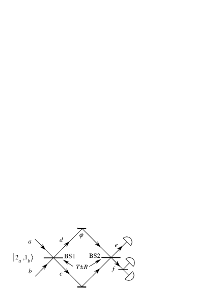
Figure 1: Arrangement of asymmetric beam splitters of a three-photon interferometer for the demonstration of the three-photon de Broglie wavelength.

II.2 Experiment

Experimentally, asymmetric beam splitters are realized via polarization projections as shown in Fig.2 and its inset (a), where a three-photon state of $|2_{H},1_{V}\rangle$ is incident on a combination of two half wave plates (HWP1, HWP2) and a phase retarder (PS). The first half wave plate (HWP1) rotates the state $|2_{H},1_{V}\rangle$ by an angle $\alpha$ to $|2_{a},1_{b}\rangle$ with

$$\begin{cases}\hat{a}_{H}=\hat{a}\cos\alpha+\hat{b}\sin\alpha,\cr\hat{a}_{V}=\hat{b}\cos\alpha-\hat{a}\sin\alpha,\end{cases}$$ (11)

where $\cos\alpha=\sqrt{T}=1/\sqrt{3}$ is the amplitude transmissivity of the asymmetric beam splitter. Eq.(11) is equivalent to Eq.(7). The phase retarder (PS) introduces the phase shift $\varphi$ between the H and V polarization. The second half wave plate (HWP2) makes another rotation of the same angle $\alpha$ for the two phase-shifted polarizations and the polarization beam splitter finishes the projection required by Eq.(8).

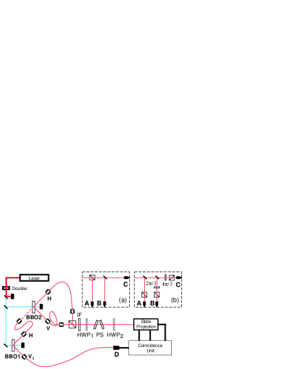
Figure 2: Experimental setup. HWP1 and HWP2 is set for different measurement, PS is the phase shifter between H-photon and V-photon. Insets: (a) arrangement with asymmetric beam splitters by polarization beam splitter (PBS) and (b) the three-photon NOON state projection.

The three-photon polarization state of $|2_{H},1_{V}\rangle$ is prepared by using two type-II parametric down conversion processes shown in Fig.2. This scheme was first constructed by Liu et al liu to demonstrate controllable temporal distinguishability of three photons. When the delay between the two H-photons is zero, we have the state of $|2_{H},1_{V}\rangle$. In this scheme, two $\beta$-Barium Borate (BBO) crystals are pumped by two UV pulses from a common source of frequency doubled Ti:sapphire laser operating at 780 nm. The H-photon from BBO1 is coupled to the H-polarization mode of BBO2 while the other V-photon is detected by detector D and serves as a trigger. The H- and V-photons from BBO2 are coupled to single-mode fibers and then are combined by a polarization beam splitter (PBS). The combined fields pass through an interference filter with 3 nm bandwidth and then go to the assembly of HWP1, PS, and HWP2 to form a three-photon polarization interferometer. There are two schemes of projection measurement. In this section, we deal with the first scheme in inset (a) of Fig.2, which consists of a PBS for projection and three detectors (A, B, C) for measuring the quantity $P_{3}(1_{e},2_{f})$ in Eq.(6) by three-photon coincidence. To realize the transformation in Eqs.(7, 8), HWP1 and HWP2 are set to rotate the polarization by $\alpha=\cos^{-1}(1/\sqrt{3})=54.7^{\circ}$. In order to obtain an input state of $|2_{H},1_{V}\rangle$ to the interferometer, we need to gate the three-photon coincidence measurement on the detection at detector D. In this way, we ensure that the two H-photons come from two crystals separately. Otherwise, we will have an input state of $|2_{H},2_{V}\rangle$. The delay ($\Delta T_{H}$) between the two H-photons from BBO1 and BBO2 as well as the delay ($\Delta T_{V}$) between the H- and V-photons are adjusted to insure the three photons are indistinguishable in time. This is confirmed by the photon bunching effect of the two H-photons liu and a generalized Hong-Ou-Mandel effect for three photons san .

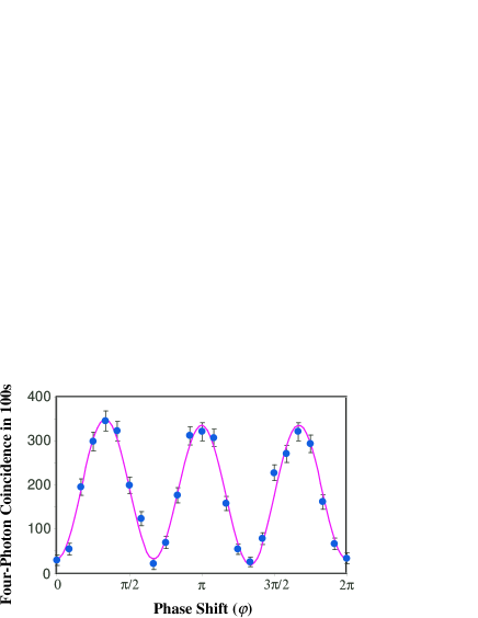
Figure 3: Experimental result for projection measurement with asymmetric beam splitters. The data is least-square-fitted to $P_{40}(1+{\cal V}_{3}\cos 3\varphi+{\cal V}_{1}\cos\varphi)$ with ${\cal V}_{3}=85\%$ and ${\cal V}_{1}=5\%$ after background subtraction.

Four-photon coincidence count among ABCD detectors is measured as a function of the phase shift $\varphi$. The experimental result after background subtraction is shown in Fig.3. The data is gathered in 100 sec for each point and the error bars are one standard deviation. Backgrounds due to three and more pairs of photons are estimated from single and two-photon rates to contribute 1.2/sec on average to the raw data and are subtracted. The data clearly show a $\cos 3\varphi$ dependence except the unbalanced minima and maxima, which indicates an extra $\cos\varphi$ dependence. Indeed, the data fit well to the function

$$P_{4}=P_{40}(1+{\cal V}_{3}\cos 3\varphi+{\cal V}_{1}\cos\varphi)$$ (12)

with $P_{40}=184$, ${\cal V}_{3}=85\%$ and ${\cal V}_{1}=5\%$. The $\chi^{2}$ of the fit is 30 and is comparable to the number of data of 25, indicating a mostly statistical cause for the error.

The appearance of the $\cos\varphi$ term in Eq.(12) is an indication that the cancellation of the $|2_{c},1_{d}\rangle$ and $|1_{c},2_{d}\rangle$ is not complete in Eqs.(4, 10) and the residuals mix with the $|3_{c},0_{d}\rangle$ and $|0_{c},3_{d}\rangle$ terms to produce the $\cos\varphi$ term. This imperfect cancellation is not a result of the wrong $T,R$ values but is due to temporal mode mismatch among the three photons in the input state of $|2_{H},1_{V}\rangle$. To account for this mode mismatch, we resort to a multi-mode model of the parametric down-conversion process.

II.3 Multi-mode analysis of three-photon interferometer with asymmetric beam splitters

We start by finding the multi-mode description of the quantum state from two parametric down-conversion processes. Since the first one serves as the input to the second one, we need the evolution operator for the process, which was first dealt with by Ghosh et al gho and later by Ou ou4 and by Grice and Walmsley wam . In general, the unitary evolution operator for weakly pumped type-II process is given by

$$\hat{U}=1+\eta\int d\omega_{1}d\omega_{2}\Phi(\omega_{1},\omega_{2})\hat{a}_{H}^{{\dagger}}(\omega_{1})\hat{a}_{V}^{{\dagger}}(\omega_{2}),$$ (13)

where $\eta$ is some parameter that is proportional to the pump strength and nonlinear coupling. For simplicity without losing generality, we assume the two processes are identical and are governed by the evolution operator in Eq.(13). Furthermore, we assume the symmetry relation $\Phi(\omega_{1},\omega_{2})=\Phi(\omega_{2},\omega_{1})$ which is in general not satisfied but can be achieved with some symmetrizing tricks wam2 ; wong . So for the first process, because the input is vacuum, we obtain the output state as

$$|\Psi_{1}\rangle=\hat{U}|vac\rangle=|vac\rangle+\eta\int d\omega_{1}d\omega_{2}\Phi(\omega_{1},\omega_{2})\hat{a}_{H}^{{\dagger}}(\omega_{1})\hat{a}_{V}^{{\dagger}}(\omega_{2})|vac\rangle.$$ (14)

The second crystal has the state of $|\Psi_{1}\rangle$ as its input. So after the second crystal, the output state becomes

$$|\Psi_{2}\rangle=\hat{U}|\Psi_{1}\rangle=...+\eta^{2}\int d\omega_{1}d\omega_{2}d\omega_{1}^{\prime}d\omega_{2}^{\prime}\Phi(\omega_{1},\omega_{2})\Phi(\omega_{1}^{\prime},\omega_{2}^{\prime})\hat{a}_{H}^{{\dagger}}(\omega_{1}^{\prime})\hat{a}_{V}^{{\dagger}}(\omega_{2}^{\prime})\hat{a}_{H}^{{\dagger}}(\omega_{1})\hat{a}_{V_{1}}^{{\dagger}}(\omega_{2})|vac\rangle,$$ (15)

where $V_{1}$ and $V$ denote the two non-overlapping vertical polarization mode from the first and second crystals, respectively. Here we only keep the four-photon term. Although there are other four-photon terms in the $|\Psi_{2}\rangle$ state corresponding to two-pair generation from one crystal alone, they won’t contribute to what we are going to calculate. So we omit them in Eq.(15).

The field operators at the four detectors are given by

$$\begin{cases}\hat{E}_{A}(t)=\tau_{1}\hat{E}_{H}(t)+\rho_{1}\hat{E}_{V}(t),\cr\hat{E}_{B}(t)=\big{[}\tau_{2}\hat{E}_{V}(t)+\rho_{2}\hat{E}_{H}(t)\big{]}/\sqrt{2}+...=\hat{E}_{C}(t),\end{cases}$$ (16)

with $\tau_{1}=(1-2e^{i\varphi})/3,\tau_{2}=(e^{i\varphi}-2)/3,\rho_{1}=-\rho_{2}=\sqrt{2}(1+e^{i\varphi})/3$. Here we used the equivalent relations in Eqs.(7, 8) to establish the connection between the field operators $\hat{E}_{A},\hat{E}_{B},\hat{E}_{C}$ and $\hat{E}_{H},\hat{E}_{V}$ and for detector D, we have

$$\hat{E}_{D}(t)=\hat{E}_{V_{1}}(t),$$ (17)

with

$$\hat{E}_{k}(t)={1\over\sqrt{2\pi}}\int d\omega\hat{a}_{k}(\omega)e^{-i\omega t}.~{}~{}~{}~{}~{}(k=H,V,V_{1})$$ (18)

The four-photon coincidence rate of ABCD is proportional to a time integral of the correlation function

$$\Gamma^{(4)}(t_{1},t_{2},t_{3},t_{4})=\langle\Psi_{2}|\hat{E}_{D}^{{\dagger}}(t_{4})\hat{E}_{C}^{{\dagger}}(t_{3})\hat{E}_{B}^{{\dagger}}(t_{2})\hat{E}_{A}^{{\dagger}}(t_{1})\hat{E}_{A}(t_{1})\hat{E}_{B}(t_{2})\hat{E}_{C}(t_{3})\hat{E}_{D}(t_{4})|\Psi_{2}\rangle.$$ (19)

It is easy to first evaluate $\hat{E}_{A}(t_{1})\hat{E}_{B}(t_{2})\hat{E}_{C}(t_{3})\hat{E}_{D}(t_{4})$:

$$\hat{E}_{A}(t_{1})\hat{E}_{B}(t_{2})\hat{E}_{C}(t_{3})\hat{E}_{D}(t_{4})=\big{[}(HHV+HVH)D\tau_{1}\tau_{2}\rho_{2}+VHHD\rho_{1}\rho_{2}^{2}\big{]}/2+...,$$ (20)

where $H=\hat{E}_{H}$, $V=\hat{E}_{V}$, $D=\hat{E}_{D}$ for short and we keep the time ordering of $t_{1}t_{2}t_{3}$. We also drop five terms that give zero result when they operate on $|\Psi_{2}\rangle$. It is now straightforward to calculate the quantity $\hat{E}_{A}(t_{1})\hat{E}_{B}(t_{2})\hat{E}_{C}(t_{3})$ $\hat{E}_{D}(t_{4})|\Psi_{2}\rangle$, which has the form of

$$\hat{E}_{A}(t_{1})\hat{E}_{B}(t_{2})\hat{E}_{C}(t_{3})\hat{E}_{D}(t_{4})|\Psi_{2}\rangle={\eta^{2}\over 2}\Big{\{}\big{[}G(t_{1},t_{2},t_{3},t_{4})+G(t_{2},t_{1},t_{3},t_{4})+G(t_{1},t_{3},t_{2},t_{4})+G(t_{3},t_{1},t_{2},t_{4})\big{]}\tau_{1}\tau_{2}\rho_{2}$$ (21)

$$\hskip 216.81pt+\big{[}G(t_{2},t_{3},t_{1},t_{4})+G(t_{3},t_{2},t_{1},t_{4})\big{]}\rho_{1}\rho_{2}^{2}\Big{\}}|vac\rangle,$$ (22)

where

$$G(t_{1},t_{2},t_{3},t_{4})=g(t_{1},t_{3})g(t_{2},t_{4})~{}~{}~{}~{}{\rm with}~{}~{}~{}g(t,t^{\prime})\equiv{1\over 2\pi}\int d\omega_{1}d\omega_{2}\Phi(\omega_{1},\omega_{2})e^{-i(\omega_{1}t+\omega_{2}t^{\prime})}.$$ (23)

Substituting Eq.(22) into Eq.(19) and carrying out the time integral, we obtain

$$P_{4} \propto \int dt_{1}dt_{2}dt_{3}dt_{4}\Gamma^{(4)}(t_{1},t_{2},t_{3},t_{4})$$ (24)

$$= {|\eta|^{4}\over 4}\int d\omega_{1}d\omega_{2}d\omega_{1}^{\prime}d\omega_{2}^{\prime}\Big{|}\big{[}\Phi(\omega_{1},\omega_{2})\Phi(\omega_{1}^{\prime},\omega_{2}^{\prime})+\Phi(\omega_{1},\omega_{1}^{\prime})\Phi(\omega_{2},\omega_{2}^{\prime})\big{]}(\tau_{1}\tau_{2}\rho_{2}+\rho_{1}\rho_{2}^{2})$$ (26)

$$\hskip 216.81pt+2\Phi(\omega_{1}^{\prime},\omega_{2})\Phi(\omega_{1},\omega_{2}^{\prime})\tau_{1}\tau_{2}\rho_{2}\Big{|}^{2}.$$

With $\tau_{1},\rho_{1},\tau_{2},\rho_{2}$, we can further reduce Eq.(26) to

$$P_{4}\propto{2|\eta|^{4}(17{\cal A}+7{\cal E})\over 243}\Big{[}1+{\cal V}_{3}\cos 3\varphi+{\cal V}_{1}\cos\varphi\Big{]}$$ (27)

where

$${\cal V}_{3}={8({\cal A}+2{\cal E})\over 17{\cal A}+7{\cal E}},~{}~{}~{}{\cal V}_{1}={9({\cal A}-{\cal E})\over 17{\cal A}+7{\cal E}}.$$ (28)

and

$${\cal A}=\int d\omega_{1}d\omega_{2}d\omega_{1}^{\prime}d\omega_{2}^{\prime}|\Phi(\omega_{1},\omega_{2})\Phi(\omega_{1}^{\prime},\omega_{2}^{\prime})|^{2}$$ (29)

$${\cal E}=\int d\omega_{1}d\omega_{2}d\omega_{1}^{\prime}d\omega_{2}^{\prime}\Phi^{*}(\omega_{1},\omega_{2})\Phi^{*}(\omega_{1}^{\prime},\omega_{2}^{\prime})$$ (30)

$$\hskip 108.405pt\times\Phi(\omega_{1}^{\prime},\omega_{2})\Phi(\omega_{1},\omega_{2}^{\prime}).~{}~{}~{}~{}~{}$$ (31)

In deducing Eqs.(26–31), we used the symmetry relation $\Phi(\omega_{1},\omega_{2})=\Phi(\omega_{2},\omega_{1})$.

Obviously, when ${\cal A}={\cal E}$, Eq.(27) completely recovers to Eq.(10). In practice, we always have ${\cal A}\geq{\cal E}$ by Schwartz inequality. When ${\cal E}<{\cal A}$, Eq.(27) has the same form as Eq.(12), indicating that the multi-mode analysis indeed correctly predicts the imperfect cancellation of the $|2_{H},1_{V}\rangle$ and $|2_{V},1_{H}\rangle$ terms in Eqs.(4, 10). If we use the experimentally measured ${\cal V}_{3}$ and ${\cal V}_{1}$ in Eq.(28), we will obtain two inconsistent values of ${\cal E}/{\cal A}$: $({\cal E}/{\cal A})_{3}=0.65$ and $({\cal E}/{\cal A})_{1}=0.87$. The discrepancy is the result of the break up of the symmetry relation of $\Phi(\omega_{1},\omega_{2})=\Phi(\omega_{2},\omega_{1})$ for type-II parametric down-conversion, which is reflected in the less-than-unit visibility of the two-photon interference. This imperfection can be modelled as spatial mode mismatch and approximately modifies Eq.(28) as

$${\cal V}_{3}=v_{1}^{3}{8({\cal A}+2{\cal E})\over 17{\cal A}+7{\cal E}},~{}~{}~{}{\cal V}_{1}=v_{1}{9({\cal A}-{\cal E})\over 17{\cal A}+7{\cal E}},$$ (32)

where $v_{1}$ is the equivalent reduced visibility in single-photon interference due to spatial mode mismatch. With the extra parameter $v_{1}$ in Eq.(32), we obtain a consistent $({\cal E}/{\cal A})=0.86$ with $v_{1}=0.96$.

III NOON state projection measurement

The projection measurement discussed in the previous section relies on the cancellation of some specific terms and therefore cannot be applied to an arbitrary photon number. In the following, we will discuss another projection scheme that can cancel all the unwanted terms at once and thus can be scaled up.

III.1 Principle of experiment

The NOON-state projection measurement scheme was first proposed by Sun et al sun1 and realized by Resch et al res for six-photon case and by Sun et al sun2 for the four-photon case. Since it is based on a multi-photon interference effect, it was recently used to demonstrate the temporal distinguishability of an N-photon state xia ; ou5 . Here we will apply it to a three-photon superposition state for the demonstration of three-photon de Broglie wave length without the NOON state.

The NOON-state projection measurement scheme for three-photon case is sketched in inset (b) of Fig.1. In this scheme, the input field is first divided into three equal parts. Then each part passes through a phase retarder that introduces a relative phase difference of $0,2\pi/3,4\pi/3$ respectively between the H- and V-polarization. The phase shifted fields are then projected to $135^{\circ}$ direction by polarizers before being detected by A, B, C detectors, respectively. It was shown that the three-photon coincidence rate is proportional to

$$P_{3}\propto{1\over 18}\Big{|}\langle NOON_{3}|\Phi_{3}\rangle\Big{|}^{2},$$ (33)

where $|NOON_{3}\rangle=(|3_{H},0_{V}\rangle-|0_{H},3_{V}\rangle)/\sqrt{2}$ and $|\Phi_{3}\rangle=c_{0}|3_{H},0_{V}\rangle+c_{1}|2_{H},1_{V}\rangle+c_{2}|1_{H},2_{V}\rangle+c_{3}|0_{H},3_{V}\rangle$. Note that since $|2,1\rangle,|1,2\rangle$ are orthogonal to the NOON-state, their contributions to $P_{3}$ are zero. Assuming that $|c_{0}|=|c_{3}|=c$ and there is a relative phase of $\varphi$ between H and V so that $c_{0}=c,c_{3}=ce^{i3\varphi}$, we obtain from Eq.(33)

$$P_{3}\propto{|c|^{2}\over 18}(1-\cos 3\varphi),$$ (34)

which is exactly in the form of Eq.(2) with $N=3$, showing the three-photon de Broglie wave length.

III.2 Experiment

From Sect.IIB, we learned that a state of $|2_{H},1_{V}\rangle$ can be produced with two parametric down-conversion processes. This state will of course give no contribution to the NOON state projection since it is orthogonal to the NOON state. On the other hand, we can rotate the state by 45^∘. Then the state becomes ou3 ; cam

$$|\Phi_{3}\rangle=\sqrt{3\over 8}\Big{(}|3_{H},0_{V}\rangle-|0_{H},3_{V}\rangle\Big{)}$$ (35)

$$\hskip 72.26999pt+{1\over\sqrt{8}}\Big{(}|2_{H},1_{V}\rangle-|1_{H},2_{V}\rangle\Big{)},~{}~{}~{}~{}~{}~{}$$ (36)

which has the NOON state component with $c=\sqrt{3/8}$.

Experimentally, the three-photon state of $|2_{H},1_{V}\rangle$ is prepared in the same way described in Sect.IIB and shown in Fig.2. Different from Sect.IIB, the polarizations of the prepared state are rotated 45^∘ by HWP1 to achieve the state in Eq.(36). The phase shifter (PS) then introduces a relative phase difference $\varphi$ between the H and V polarizations and HWP2 is set at zero before the NOON state projection measurement is performed [Inset (b) of Fig.2]. As before, a four-photon coincidence measurement among ABCD detectors is equivalent to a three-photon coincidence measurement by ABC detectors gated on the detection at D, which is required for the production of $|2_{H},1_{V}\rangle$.

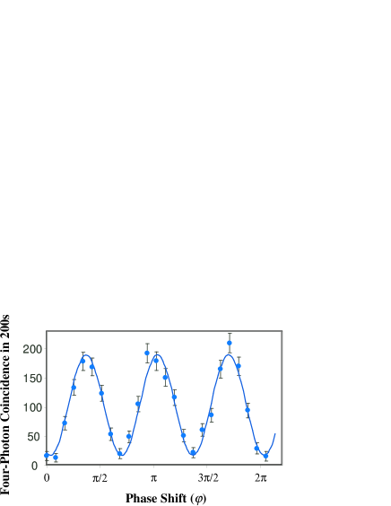
Figure 4: Experimental result for the NOON state projection measurement. The data is least-square-fitted to $P_{40}(1+{\cal V}_{3}\cos 3\varphi$ with ${\cal V}_{3}=84\%$ after background subtraction.

Four-photon coincidence count among ABCD detectors is registered in 200 sec as a function of the phase $\varphi$ (PS). The data after subtraction of background contributions is plotted in Fig.4. It clearly shows a sinusoidal dependence on $\varphi$ with a period of $2\pi/3$. The solid curve is a chi-square fit to the function of $P_{4}=P_{40}[1+{\cal V}_{3}\cos 3(\varphi+\varphi_{0})]$ with $P_{40}=103/200$sec and ${\cal V}_{3}=0.84$. The $\chi^{2}$ of the fit is 24.3, which is comparable to the number of data of 25 indicating a good statistical fit.

The less-than-unit visibility is a result of temporal distinguishability among the three photons produced from two crystals. It can only be accounted for with a multi-mode model of the state given in Sect.IIC. Let’s now apply it to the current scheme.

III.3 Multi-mode analysis

The input state is same as Eq.(15). But the field operators are changed to

$$\begin{cases}\hat{E}_{A}(t)=\big{[}\hat{E}_{+}(t)-e^{i\varphi}\hat{E}_{-}(t)\big{]}/\sqrt{6}+...,\cr\hat{E}_{B}(t)=\big{[}\hat{E}_{+}(t)-e^{i\varphi}\hat{E}_{-}(t)e^{i2\pi/3}\big{]}/\sqrt{6}+...,\cr\hat{E}_{C}(t)=\big{[}\hat{E}_{+}(t)-e^{i\varphi}\hat{E}_{-}(t)e^{i4\pi/3}\big{]}/\sqrt{6}+...,\end{cases}$$ (37)

with

$$\begin{cases}\hat{E}_{+}(t)=\big{[}\hat{E}_{H}(t)+\hat{E}_{V}(t)\big{]}/\sqrt{2},\cr\hat{E}_{-}(t)=\big{[}\hat{E}_{H}(t)-\hat{E}_{V}(t)\big{]}/\sqrt{2},\end{cases}$$ (38)

where we omit the vacuum input fields and $\varphi$ is the phase shift introduced by PS in Fig.2. The field operator for detector D is same as Eq.(17).

As in Sect.IIC, the four-photon coincidence rate is related to the correlation function in Eq.(19) and we can first evaluate $\hat{E}_{A}(t_{1})\hat{E}_{B}(t_{2})\hat{E}_{C}(t_{3})\hat{E}_{D}(t_{4})$. With the field operators in Eq.(37), we obtained

$$\hat{E}_{A}(t_{1})\hat{E}_{B}(t_{2})\hat{E}_{C}(t_{3})\hat{E}_{D}(t_{4})$$ (39)

$$\hskip 21.68121pt=\big{(}HHVa_{1}+HVHa_{2}+VHHa_{3}\big{)}/12\sqrt{12},~{}~{}~{}~{}~{}$$ (40)

with

$$\begin{cases}a_{1}=1+e^{i3\varphi}+2e^{i(2\varphi+2\pi/3)}+2e^{i(\varphi+4\pi/3)}\cr a_{2}=1+e^{i3\varphi}+2e^{i(2\varphi+4\pi/3)}+2e^{i(\varphi+2\pi/3)}\cr a_{3}=1+e^{i3\varphi}+2e^{i2\varphi}+2e^{i\varphi},\end{cases}$$ (41)

where the notations are same as in Eq.(20) and we used the identity $1+e^{i2\pi/3}+e^{i4\pi/3}=0$. As before, we also drop five terms that give zero result when they operate on $|\Psi_{2}\rangle$. Now we can calculate the quantity $\hat{E}_{A}(t_{1})\hat{E}_{B}(t_{2})\hat{E}_{C}(t_{3})\hat{E}_{D}(t_{4})|\Psi_{2}\rangle$, which has the form of

$$\hat{E}_{A}(t_{1})\hat{E}_{B}(t_{2})\hat{E}_{C}(t_{3})\hat{E}_{D}(t_{4})|\Psi_{2}\rangle={\eta^{2}\over\sqrt{12^{3}}}\Big{\{}\big{[}G(t_{1},t_{2},t_{3},t_{4})+G(t_{2},t_{1},t_{3},t_{4})\big{]}a_{1}+\big{[}G(t_{1},t_{3},t_{2},t_{4})+G(t_{3},t_{1},t_{2},t_{4})\big{]}a_{2}$$

$$\hskip 216.81pt+\big{[}G(t_{2},t_{3},t_{1},t_{4})+G(t_{3},t_{2},t_{1},t_{4})\big{]}a_{3}\Big{\}}|vac\rangle,$$ (42)

where $G(t_{1},t_{2},t_{3},t_{4})$ is given in Eq.(23). After the time integral, we obtain

$$P_{4}(NOON)\propto{|\eta|^{4}(2{\cal A}+{\cal E})\over 72}\big{(}1+{\cal V}_{3}\cos 3\varphi\big{)}$$ (43)

with

$${\cal V}_{3}(NOON)={{\cal A}+2{\cal E}\over 2{\cal A}+{\cal E}},$$ (44)

where ${\cal A}$ and ${\cal E}$ are given in Eqs.(29, 31). Note that the terms such as $\cos 2\varphi,\cos\varphi$ are absent in Eq.(44) even in the non-ideal case of ${\cal E}<{\cal A}$. This is because of the symmetry among the three detectors A, B, C involved in the three-photon NOON state projection measurement. When spatial mode mismatch is considered, the visibility is changed to

$${\cal V}_{3}(NOON)=v_{1}^{3}{{\cal A}+2{\cal E}\over 2{\cal A}+{\cal E}}.$$ (45)

With $v_{1}$ and the quantity ${\cal E}/{\cal A}$ obtained in Sect.IIC, we have ${\cal V}_{3}(NOON)=0.85$, which is close to the observed value of 0.84 in Sect.IIIB.

IV Summary and Discussion

In summary, we demonstrate a three-photon de Broglie wavelength by using two different schemes of projection measurement without the need for a hard-to-produce NOON state. Quantum interference is responsible for the cancellation of the unwanted terms. The first scheme by asymmetric beam splitters targets specific terms while the second one by NOON state projection cancels all the unwanted terms at once. We use a multi-mode model to describe the non-ideal situation encountered in the experiment and find good agreements with the experimental results.

Since the scheme by asymmetric beam splitters is only for some specific terms, it cannot be easily scaled up to arbitrary number of photons although the extension to the four-photon case is available. The extension of the scheme by NOON state projection to arbitrary number of photons is straightforward. In fact, demonstrations with four and six photons have been done with simpler states res ; sun2 .

On the other hand, the scheme of NOON state projection need to divide the input fields into $N$ equal parts while the scheme with asymmetric beam splitters requires less partition. So the latter will have higher coincidence rate than the former. In fact, Fig.3 and Fig.4 show a ratio of 4 after pump intensity correction. This is consistent with the ratio of 4.8 from Eqs.(27, 43) when ${\cal E=A}$. The difference may come from the different collection geometry in the layout.

The dependence of the visibility in Eqs.(32, 44) on the quantity ${\cal E/A}$ reflects the fact that the interference effect depends on the temporal indistinguishability of the three photons. From previous studies ou6 ; tsu ; ou7 ; sun1 ; liu , we learned that the quantity ${\cal E/A}$ is a measure of indistinguishability between two pairs of photons in parametric down-conversion. In our generation of the $|2_{H},1_{V}\rangle$ state, one of the H-photon is from another pair of down-converted photons. So to form an indistinguishable three-photon state, we need pair indistinguishability, i.e., ${\cal E/A}\rightarrow 1$.

- (1) J. Jacobson, G. Björk, I. Chuang and Y. Yamamoto, Phys. Rev. Lett. 74, 4835 (1995).
- (2) W. Heisenberg, Zeitschr. f. Physik 43, 172 (1927).
- (3) M. J. Holland and K. Burnett, Phys. Rev. Lett. 71, 1355 (1993).
- (4) J. J. Bollinger, W. M. Itano, D. J. Wineland, and D. J. Heinzen, Phys. Rev. A54, R4649 (1996).
- (5) Z. Y. Ou, Phys. Re. Lett. 77, 2352 (1996); Phys. Rev. A 55, 2598 (1997).
- (6) A. N. Boto, P. Kok, D. S. Abrams, S. L. Braunstein, C. P. Williams, and J. P. Dowling, Phys. Rev. Lett. 85, 2733 (2000); P. Kok, A. N. Boto, D. S. Abrams, C. P. Williams, S. L. Braunstein, and J. P. Dowling, Phys. Rev. A63, 063407 (2001).
- (7) Z. Y. Ou, X. Y. Zou, L. J. Wang, and L. Mandel, Phys. Rev. A 42, 2957 (1990).
- (8) J. G. Rarity, P. R. Tapster, E. Jakeman, T. Larchuk, R. A. Campos, M. C. Teich, and B. E. A. Saleh, Phys. Rev. Lett. 65, 1348 (1990).
- (9) H. F. Hofmann, Phys. Rev. A 70, 023812 (2004).
- (10) F. Shafiei, P. Srinivasan, and Z. Y. Ou, Phys. Rev. A 70, 043803 (2004).
- (11) B. Liu and Z. Y. Ou, Phys. Rev. A 74, 035802 (2006).
- (12) P. Walther, J. W. Pan, M. Aspelmeyer, R. Ursin, S. Gasparoni, and A. Zeilinger, Nature (London) 429, 158 (2004).
- (13) M. W. Mitchell, J. S. Lundeen, and A. M. Steinberg, Nature (London) 429, 161 (2004).
- (14) H. B. Wang, and T. Kobayashi, Phys. Rev. A 71, 021802(R) (2005).
- (15) F. W. Sun, Z. Y. Ou, and G. C. Guo, Phys. Rev. A 73, 023808 (2006).
- (16) K. J. Resch, K. L. Pregnell, R. Prevedel, A. Gilchrist, G. J. Pryde, J. L. O’Brien, and A. G. White, quant-ph/0511214.
- (17) F. W. Sun, B. H. Liu, Y. F. Huang, Z. Y. Ou, and G. C. Guo, Phys. Rev. A 74, 033812 (2006).
- (18) K. Sanaka, K. J. Resch, and A. Zeilinger, Phys. Rev. Lett. 96, 083601 (2006).
- (19) C.K. Hong, Z.Y. Ou, and L. Mandel, Phys. Rev. Lett. 59, 2044 (1987).
- (20) Z. Y. Ou, C. K. Hong, and L. Mandel, Opt. Commun. 63, 118 (1987).
- (21) R. A. Campos, B. E. A. Saleh, and M. C. Teich, Phys. Rev. A 40, 1371 (1989).
- (22) L. Mandel and E. Wolf, Optical Coherence and Quantum Optics, (Cambridge University Press, New York, 1995).
- (23) B. H. Liu, F. W. Sun, Y. X. Gong, Y. F. Huang, Z. Y. Ou, and G. C. Guo, quant-ph/0606118.
- (24) R. Ghosh, C. K. Hong, Z. Y. Ou, and L. Mandel, Phys. Rev. A34, 3962 (1986).
- (25) Z. Y. Ou, Quan. Semiclass. Opt. 9 599 (1997).
- (26) W. P. Grice and I. A. Walmsley, Phys. Rev. A 56, 1627 (1997).
- (27) D. Branning, W. P. Grice, R. Erdmann, and I. A. Walmsley, Phys. Rev. Lett. 83, 955 (1999)
- (28) O. Kuzucu, M. Fiorentino, M. A. Albota, F. N. C. Wong, and F. X. Kärtner, Phys. Rev. Lett. 94, 083601 (2005).
- (29) Z. Y. Ou, quant-ph/0601118.
- (30) G. Y. Xiang, Y. F. Huang, F. W. Sun, P. Zhang, Z. Y. Ou, and G. C. Guo, Phys. Rev. Lett. 97, 023604 (2006).
- (31) Z. Y. Ou, J. K. Rhee, and L. J. Wang, Phys. Rev. A 60, 593 (1999).
- (32) K. Tsujino, H. F. Hofmann, S. Takeuchi, and K. Sasaki, Phys. Rev. Lett. 92, 153602 (2004).
- (33) Z. Y. Ou, Phys. Rev. A 72, 053814 (2005).