Chapter 1 Introduction

Are you entangled?

1.1 Overview and Objectives

In the last two decades quantum information theory has emerged as a branch of quantum physics which links concepts of quantum physics to ideas from information theory. On the one hand it became evident that the language from classical information theory is appropriate to grasp several important open questions in quantum mechanics. On the other hand, it was recognised that quantum mechanical systems would allow for processing of classical information that could not be realised with physical systems belonging to the realm of classical physics. Most prominently perhaps, factoring of large numbers is a problem that can be solved in polynomial time on a quantum computer. In computer science, this problem belongs to the complexity class of NP problems, which means that there is no known polynomial time algorithm for a classical computer. Frankly, to factor large numbers is simply not possible in any reasonable time scale with a classical computer. The insight that there exist quantum algorithms that so massively outperform the best known classical algorithms resulted in a strong interest in quantum computation. Soon other subjects of information theory were reviewed from the quantum physics perspective, and many other applications were found.

Furthermore it was recognised that entanglement plays a major role for those applications which can not be realised with classical schemes or setups. Today, entanglement is seen as a resource, which is consumed when using it for quantum information processing. The dictionary describes entangled as follows:

If something is entangled in something else, such as a rope, wire, or net, it is caught in it very firmly.

If you are entangled in something, you are involved in difficulties from which it is hard to escape.

If you are entangled with someone, you are involved in a relationship with them that causes problems or difficulties.

In quantum physics, entangled states can be understood as states where degrees of freedom of parts of the system are tightly correlated. In contrast to classical correlations, entanglement can not be generated by a preparation using only local operations on parts of the system and thus offers new dimensions for information theory and leads to manifestly counterintuitive consequences. Since entanglement is the necessary ingredient for so many applications, one naturally wants to know how to quantify it. Different entanglement measures were proposed, and the concepts of distillable entanglement and entanglement cost were introduced.

Until recently, research in the field of the theory of entanglement and its applications has almost exclusively dealt with finite dimensional quantum systems such as two-level systems, in analogy to the classical bits called qubits. The theoretical concept of two-level systems can be realised in nature by the two directions of a spin in a magnetic field or by the polarisation degrees of freedom of light. It was, for example, shown that teleportation of an unknown two-level state between two parties is possible, if both share a pair of entangled states. The experimental realisation was done in 1998, Ref. [4].
Discrete systems, like the two-level systems, are associated with finite-dimensional Hilbert spaces. In recent years, continuous variable systems (CVS) came into the focus of research and fruitful attempts were done to employ the concepts and insights from discrete systems on continuous variable states, living in an infinite dimensional Hilbert space. Examples are the quantised electromagnetic field, known as a set of harmonic oscillators, the vibrational degree of freedom of ions in a trap, or mechanical oscillators in the quantum domain. The simplest nontrivial yet very important class of CVS are the Gaussian states determined by their first and second moments alone. They show most of the interesting effects like entanglement and squeezing and are mathematically easy to handle. Furthermore Gaussian states are experimentally available in optical settings.

We will investigate the entanglement properties of Gaussian states and formulate them on covariance matrices, associated to the states. Furthermore, we do not only want to quantify the degree of entanglement, but also to estimate how much a given state is entangled. This question is not easy to answer even in the case when the state is fully known, but additionally one is interested in good strategies of how to estimate or give a minimum amount of entanglement of an unknown or partly known state. The young theory of entanglement witnesses is introduced and provides a powerful tool to answer this question. As we will present in the sixth chapter, it is indeed possible to use entanglement witnesses in order to estimate the degree of entanglement of an unknown state with experimentally available measurements. To quantify entanglement we will throughout this thesis use the logarithmic negativity, being so far the only computable entanglement measure for general states.

1.2 Outline

This thesis is divided in seven chapters, and an appendix collecting some small definitions and proofs. The material is organised as follows:

Basics

In this chapter several concepts of continuous variable quantum mechanics are reviewed, namely the commutation relations, the concept of phase space and of canonical (symplectic) transformations. We introduce the moments of a state and the quantum analogue to the classical characteristic function. Finally, we define entanglement and state the famous PPT-criterion.

Gaussian States

In the third chapter we introduce the set of Gaussian states starting with some familiar examples as the coherent states of a harmonic oscillator. We define the covariance matrix as the major quantity determining most of the important properties of a Gaussian state. Furthermore two useful normal forms of covariance matrices will be introduced connected to invariant quantities, the symplectic eigenvalues and the Simon invariants, whose properties we will analyse. Additionally we see that the Gaussian states maximise the entropy.

Gaussian Operations

This chapter mainly focuses on homodyne measurements but also shortly discusses the allowed operations one could perform on a Gaussian state without destroying this property. We show that there exists an efficient setup to project an arbitrary state on a coherent state using homodyne measurements and other Gaussian operations. As we see in the subsequent chapter, the derived setup is necessary for our scheme to determine the degree of entanglement.

Measuring Entanglement of Two-Mode States

In this and the subsequent chapter the methods of estimating the degree of entanglement are introduced. First, we present a scheme of how to measure the degree of entanglement of an unknown quantum state. We propose a setup to give the exact logarithmic negativity of a Gaussian two-mode state with only nine kinds of measurements instead of estimating all entries of the covariance matrix with homodyne detections.

Entanglement Witnesses

In this chapter we introduce the theory of entanglement witnesses and show that it is a helpful tool to answer our question for entanglement properties of states. We notice that the required measurements are easily available in the laboratory and show that it is possible not only to decide experimentally whether an unknown given state is entangled or not, but also to give a lower bound of its logarithmic negativity. To do this we introduce the new quantities $p-$separability and minimal entanglement witness, which characterise the entanglement properties of covariance matrices. Finally, we present a general strategy to estimate the degree of entanglement of an unknown Gaussian state, using the concept of entanglement witnesses. As the closing words, we give an example and shortly discuss the Duan-criterion as a special case of the general criterion we stated.

Summary and Outlook

We finally summarise the main results of this thesis and give some possible issues of further research.

Chapter 2 Basics

In this thesis we will discuss aspects of quantum information theory (QIT) with continuous variable states - especially Gaussian states. These states can be described in a different formalism than the one of the familiar discrete qubit systems. We therefore start off with some basic concepts for continuous variable states (CVS).

2.1 Commutation Relations

In classical mechanics a system is described completely by its degrees of freedom, usually the coordinates ($x_{n}$) and momenta ($p_{n}$) of all $N$ particles (with $n=1,...,N$ in one-dimensional space). These canonical variables fulfil the canonical relations

$$\{R_{i},R_{j}\}=\sigma_{ij}$$ (2.1)

where $\{~{},~{}\}$ denotes the Poisson bracket defined in Def. A.1, with $R\in\mathbbm{R}^{2N}$ being the vector of canonical variables $R=(x_{1},p_{1},~{}...~{},x_{N},p_{N})^{T}$ and $\sigma$ the symplectic matrix defined as:

$$\sigma=\bigoplus_{i=1}^{N}\left(\begin{array}[]{rr}0&1\\ -1&0\end{array}\right)=\left(\begin{array}[]{rrrrrr}0&1&..&..&0&0\\ -1&0&..&..&0&0\\ ..&..&..&..&..&..\\ ..&..&..&..&..&..\\ 0&0&..&..&0&1\\ 0&0&..&..&-1&0\end{array}\right).$$ (2.2)

The phase space $(\mathbbm{R}^{2N},\sigma)$ spanned by the canonical coordinates is then a symplectic vector space (see Def. A.2) with a symplectic scalar product

$$(\xi,\eta):=\sigma(\xi,\eta)=\eta^{T}\sigma\xi=-\sigma(\eta,\xi),\quad\mbox{ for }\xi,\eta\in\mathbbm{R}^{2N},$$

which is preserved under symplectic basis transformations, defined in the next section. All $\sigma$ appearing in this thesis denote symplectic matrices of appropriate size.

In quantum mechanics we describe the canonical degrees of freedom by the set of operators $\{\hat{x}_{n},\hat{p}_{n}\}_{n}$ or equivalently by the set of ladder operators $\{\hat{a}_{n},\hat{a}^{{\dagger}}_{n}\}_{n}$ with $n=1,\ldots,N$. The generalised position operators $\hat{x}_{n}$ act in the position representation on a vector $\psi\in\mathcal{H}$ as multiplications

$$\hat{x}_{n}~{}\psi(x)=x_{n}~{}\psi(x)$$

while the generalised momentum operators $\hat{p}_{n}$ act as derivatives

$$\hat{p}_{n}~{}\psi(x)=-i~{}{\partial\psi(x)\over\partial x_{n}}.$$

These are unbounded linear, selfadjoint operators on the Hilbert space $\mathcal{H}=\mathcal{L}^{2}(\mathbbm{R}^{N},\mathbbm{C})$. When quantising a system the Poisson brackets translate to commutators and the classical canonical relations become the canonical commutation relations (CCRs):

$$[\hat{R}_{j},\hat{R}_{k}]=i\sigma_{jk}\,\hat{\mathbbm{1}}$$ (2.3)

with $\hat{R}=(\hat{R}_{1},~{}...~{},\hat{R}_{2N})^{T}=(\hat{x}_{1},\hat{p}_{1},~{}...~{},\hat{x}_{N},\hat{p}_{N})^{T}$ and $\sigma$ being the symplectic matrix. Sometimes we will also use the ladder operators, connected to the position and momentum operators via

$$\hat{a}_{n}:=\frac{\hat{x}_{n}+i\hat{p}_{n}}{\sqrt{2}} \hat{a}^{{\dagger}}_{n}:=\frac{\hat{x}_{n}-i\hat{p}_{n}}{\sqrt{2}},$$ and (2.4)

$$\hat{x}_{n}=\frac{\hat{a}_{n}+\hat{a}^{{\dagger}}_{n}}{\sqrt{2}} \hat{p}_{n}=\frac{\hat{a}_{n}-\hat{a}^{{\dagger}}_{n}}{i\sqrt{2}},$$ and (2.5)

and the translated CCRs read $[\hat{a}_{j},\hat{a}^{{\dagger}}_{k}]=\delta_{jk}\,\hat{\mathbbm{1}}$, with all other commutators equal to zero.

2.2 Symplectic Transformations

When changing our coordinate system or doing any transformation on a quantum mechanical state we use canonical transformations, $T:\hat{R}\mapsto\hat{R}^{\prime}$, which leave the basic kinematic relations unchanged, e.g., they leave the CCRs unchanged: $[\hat{R}^{\prime}_{j},\hat{R}^{\prime}_{k}]=i\,\sigma_{jk}\hat{\mathbbm{1}}$. Apart from shifts of the coordinate system’s origin the simplest canonical transformations are linear homogeneous ones. These are called symplectic transformations (see Ref. [5, 6, 7]) which form the real symplectic group, being one of the three major semisimple Lie groups besides the real orthogonal groups and the complex unitary groups.

Definition 2.1

The symplectic group will be denoted by

$$Sp(2N,\mathbbm{R})=\{S|\mbox{ real }2N\times 2N\mbox{ matrix },S\sigma S^{T}=\sigma\},$$ (2.6)

where the last condition comes from the CCRs, which shall still be fulfilled when expressing the new coordinates as linear functions of the old ones via

$$S:\hat{R}\mapsto\hat{R}^{\prime}=S\hat{R},$$ (2.7)

with $S$ being a symplectic transformation.

We find the following properties for the matrices $S\in Sp(2N,\mathbbm{R}):$

$$1. \dim(Sp(2N,\mathbbm{R}))=N(2N+1),$$

$$2. \sigma\in Sp(2N,\mathbbm{R}),$$ (2.8)

$$3. S\in Sp(2N,\mathbbm{R})\Rightarrow-S,S^{-1},S^{T}\in Sp(2N,\mathbbm{R}),$$

$$4. \det S=+1.$$

The first property comes from the restrictions on the entries of $S$ given by $S\sigma S^{T}=\sigma$, $2$ and $3$ are easy to check while the last condition is rather subtle and will be proved in the appendix (see Def. A.2 and the following discussion). Note, that all $2\times 2$ matrices with determinant one are symplectic matrices, especially all matrices from $SO(2,\mathbbm{R})$.

2.2.1 Subsets of the Symplectic Group

Sometimes it is useful to divide a symplectic transformation in transformations on subsystems. With $S=\left(\begin{array}[]{cc}A&B\\ C&D\end{array}\right)$ and $\sigma$ in a basis where $\sigma$ looks like $\sigma^{\prime}=\small\left(\begin{array}[]{cc}0&\mathbbm{1}_{N\times N}\\ -\mathbbm{1}_{N\times N}&0\end{array}\right)\normalsize,$ the properties of the symplectic $S$ may be translated to:

$$AB^{T},CD^{T},A^{T}C,B^{T}D$$ symmetric,

$$AD^{T}-BC^{T}=~{}\mathbbm{1}_{N\times N},$$ (2.9)

$$A^{T}D-C^{T}B=~{}\mathbbm{1}_{N\times N}.$$

Obviously, the symplectic transformations do in general not preserve angles between vectors. We therefore introduce the important compact, maximally complete subgroup $K(N)=Sp(2N,\mathbbm{R})\cap SO(2N)$ of $Sp(2N,\mathbbm{R})$ and find that $K(N)$ is isomorphic to the unitary group $U(N)$.

That is because every unitary $N\times N$ matrix can be expanded $U=X+iY$ where $X$ and $Y$ are real $N\times N$ matrices with

$$X^{T}X+Y^{T}Y =\mathbbm{1}_{N\times N}= XX^{T}+YY^{T},$$

$$X^{T}Y,XY^{T}$$ symmetric.

The submatrices of any $S\in K(N)$ fulfil exactly the above conditions required for any element of $U(N)$. Hence $K(N)$ is isomorphic to $U(N)$. We write the set $K(N)$ as :

$$\small{K(N)=\left\{K|K=\left(\begin{array}[]{cc}X&-Y\\ Y&X\end{array}\right)\mbox{ with }X+iY\in U(N);\,X,Y\mbox{ real}\right\}}.\normalsize$$ (2.12)

These linear homogeneous transformations will be called passive transformations because they conserve the energy of the system.

Example 1 : The two-mode (50:50) beam splitter is an element of $K(N)$.

$$S^{BS}={1\over\sqrt{2}}\left(\begin{array}[]{cc}\mathbbm{1}_{2\times 2}&-\mathbbm{1}_{2\times 2}\\ \mathbbm{1}_{2\times 2}&\mathbbm{1}_{2\times 2}.\end{array}\right)$$

Another subset of $Sp(2N,\mathbbm{R})$, although not a group, are the transformations of the form:

$$\Pi(N)=\left\{P|P\in Sp(2N,\mathbbm{R}),P=P^{T},P\geq 0\right\}.$$ (2.14)

These transformations will be called active transformations since they change the energy of the system. Generally these transformations are difficult to implement experimentally, e.g. for states of light strong nonlinear optical media are required to realise an active squeezing transformation.

Example 2 : The one-mode-squeezer changes the variances of the quadratures of a state and is an element of $\Pi(N)$.

$$S^{SQ}=\left(\begin{array}[]{cc}d&0\\ 0&{1\over d}\end{array}\right)\quad d>0\,\mbox{ is the squeezing parameter}$$

Remark: We will investigate squeezing in the subsequent chapter.

The only matrix which have both, active and passive transformations, in common is the identity matrix.

2.2.2 Normal Forms of Symplectic Transformations

We introduce some useful decompositions for symplectic matrices. For a detailed discussion see Ref. [5] and references therein.

Polar Decomposition

From matrix analysis we know that every $N\times N$ matrix $A$ can be decomposed in two matrices $P=\sqrt{A\,A^{{\dagger}}}$ and $U$ unitary, where for $A$ nonsingular $U=P^{-1}A$ is uniquely determined. If $A$ is a symplectic matrix, then $P$ and hence $U$ are real symplectic as well and $P\in\Pi(N)$ and $U\in K(N)$ by definition. Now for all $S\in Sp(2N,\mathbbm{R})$ exists a unique $P\in\Pi(N)$ and a unique $U\in K(N)$ so that $S$ can be written as a product of both:

$$S=P\,U.$$ (2.16)

The decomposition shows that every symplectic transformation can be realised by a passive transformation, like beam splitters or phase shifters, and an additional active squeezing operation.

Euler Decomposition (Singular Value Decomposition)

Since $P$ is real symmetric we may transform it orthogonally to a basis where it is diagonal: $D=O^{T}PO$ where $D$ and $O$ are again symplectic. For $D$ then follows from $D\sigma D=\sigma$ that either $\sigma_{kl}=0$ or $\lambda_{k}\lambda_{l}=1$. The diagonal matrix is thus of the form $D=\mbox{diag}(d_{1},{1\over d_{1}},...,d_{N},{1\over d_{N}})\quad\mbox{with }d_{i}>0\,\,\forall i=1,...N$.
These diagonal matrices again form a subgroup $\tilde{\Pi}(N)$ of the symplectic matrices which we name squeezing transformations or simply squeezers. We will introduce squeezed states in Section 3.1 and discuss squeezing as a property of covariance matrices in Section 3.3.

$$\tilde{\Pi}(N)=\{\tilde{P}|\tilde{P}=\mbox{diag}(d_{1},{1\over d_{1}},...,d_{N},{1\over d_{N}})\quad\mbox{with }d_{i}>0\}\subset\Pi(N)\subset Sp(2N,\mathbbm{R}).$$

We may now write every $S\in Sp(2N,\mathbbm{R})$ in the non-unique decomposition

$$S=U_{1}\,\tilde{P}\,U_{2}$$ (2.17)

with two passive transformations $U_{1},U_{2}\in K(N)$ and a squeezing transformation $\tilde{P}\in\tilde{\Pi}(N)$. The discrete non-uniqueness results from the possibility to arrange the entries of $\tilde{P}$ in different order.

Iwasawa Decomposition

The polar decomposition enables us to decompose any symplectic matrix with unique factors, but unfortunately one factor is not taken from a subgroup. The Euler decomposition allows a decomposition in subgroup factors but is not unique. We now introduce a third decomposition which unites both virtues.

The Iwasawa decomposition states that any $S\in Sp(2N,\mathbbm{R})$ can uniquely be expressed as a product of three factors

$$S=N\,\tilde{P}\,U$$ (2.18)

with $N\in\mathcal{N},\ \tilde{P}\in\tilde{\Pi}(N)$ and $U\in K(N)$ where $\mathcal{N}$ is a subgroup of $Sp(2N,\mathbbm{R})$ defined as:

$$\mathcal{N}=\left\{\left(\begin{array}[]{cc}{A}&{0}\\ {C}&{(A^{-1})^{T}}\end{array}\right)\bigg{|}{A}\,=\left(\begin{array}[]{ccc}\scriptstyle{1}&&\scriptstyle{0}\\ &\scriptstyle{\ddots}&\\ \scriptstyle{X}&&\scriptstyle{1}\end{array}\right),\,\,\scriptstyle{CA^{-1}}\mbox{ symmetric }\right\}\subset Sp(2N,\mathbbm{R}).$$

2.3 Moments

With the postulates of quantum mechanics every system can be described by an operator called density matrix or state, usually denoted by $\rho$. The density matrices provide a more convenient language for quantum mechanical systems whose state is not completely known. Additionally every such system can be completely characterised by the moments of its probability distribution, as we know it from classical statistics. In the quantum world this is the Wigner function, which is in contrast to classical statistics in general not positive. Alternatively one can use the characteristic function $\chi$, being the Fourier transformed of the Wigner function and allowing to derive the moments of the probability distribution by taking its derivatives.

Definition 2.2 (Density Matrices)

The set of density matrices (states) on a Hilbert space $\mathcal{H}$ fulfilling

$$\rho=\rho^{{\dagger}}$$ selfadjoint

$$\rho\geq 0$$ positive

$$tr[\rho]=1$$ normalised

will be denoted by $S(\mathcal{H})$. $S(\mathcal{H})$ is a closed convex subset of the bounded linear operators $\mathcal{B}(\mathcal{H})$ on $\mathcal{H}$. Note, that all states are by definition trace-class operators.

From now on all $\rho$ appearing in this thesis are elements of $S(\mathcal{H})$. The first moments of the canonical observables of a state $\rho$ are collected in the displacement vector $\vec{d}$ and can be calculated via

$$\vec{d}_{j}\quad:=\quad tr[\rho\,\hat{R}_{j}]=\langle\hat{R}_{j}\rangle,\,\quad j=1,...,2N,$$ (2.19)

while the second moments of $\rho$ are collected in the covariance matrix (CM) $\gamma$ with the relation

$$\gamma_{ij} := tr[\rho\,\{\hat{R}_{i}-\langle\hat{R}_{i}\rangle,\hat{R}_{j}-\langle\hat{R}_{j}\rangle\}_{+}]$$

$$= 2\,tr[\rho\,(\hat{R}_{i}-\langle\hat{R}_{i}\rangle)(\hat{R}_{j}-\langle\hat{R}_{j}\rangle)]-i\sigma_{ij},\,\quad i,j=1,...,2N.$$

The covariance matrix $\gamma$ of the state is a real, symmetric, $2N\times 2N$ matrix.

But not every matrix fulfilling these conditions is a proper covariance matrix, from a simple calculation we see that $\gamma$ and $\gamma+i\sigma$ (and $\gamma-i\sigma$ with complex conjugation) are necessarily positive.

Let $\gamma$ be the covariance matrix of system of $N$ modes.

$$\forall v\in\mathbbm{C}^{2N}:\quad(v|(\gamma+i\sigma)|v) = \sum_{i,j}v^{*}_{i}(\gamma_{ij}+i\sigma_{ij})v_{j}$$ (2.21)

$$= 2\,tr[\rho\sum_{i}v^{*}_{i}(\hat{R}_{i}-\langle\hat{R}_{i}\rangle)\sum_{j}v_{j}(\hat{R}_{j}-\langle\hat{R}_{j}\rangle)]$$

$$= 2\,tr[\rho\,M^{{\dagger}}M]\geq 0,$$

with $M=\sum_{j}\,v_{j}\,(\hat{R}_{j}-\langle\hat{R}_{j}\rangle)$. The right hand side is a positive number for all $v$ since $\rho$ and operators of the form $M^{{\dagger}}M$ are always positive. Therefore we find that $\gamma+i\sigma$ is positive. Similarly one shows that $\gamma\geq 0$ and $\gamma-i\sigma\geq 0$.

It turns out that the restriction $\gamma+i\sigma\geq 0$ is exactly the uncertainty relation for the canonical operators formulated in a basis independent matrix inequality (e.g., for all quadratures). Since there are no other requirements than the CCRs and the uncertainty relation, all mentioned properties of $\gamma$ are sufficient to guarantee that there exists a state $\rho\in S(\mathcal{H})$ with covariance matrix of $\gamma$ .

Example 3 : The covariance matrix of a one-mode state with vanishing displacement is:

$$\gamma=\left(\begin{array}[]{cc}2\langle\hat{x}^{2}\rangle&2\langle\hat{x}\hat{p}\rangle-i\\ 2\langle\hat{p}\hat{x}\rangle+i&2\langle\hat{p}^{2}\rangle\end{array}\right).$$

Assuming $\langle\hat{x}\hat{p}\rangle+\langle\hat{p}\hat{x}\rangle=2\langle\hat{x}\hat{p}\rangle-i=0$, the uncertainty relation on $\gamma$ reads

$$\gamma+i\sigma=\left(\begin{array}[]{cc}2\langle\hat{x}^{2}\rangle&+i\\ -i&2\langle\hat{p}^{2}\rangle\end{array}\right)\geq 0.$$

Since the trace is positive anyway the only condition to be fulfilled is a positive determinant

$$4\langle\hat{x}^{2}\rangle\langle\hat{p}^{2}\rangle-1\geq 0\quad\mbox{or }\quad\langle\hat{x}^{2}\rangle\langle\hat{p}^{2}\rangle\geq{1\over 4}.$$

But this is exactly what we know as Heisenberg uncertainty relation for the canonical coordinates.

Definition 2.3

We define the states of minimal uncertainty to be those states where half of the eigenvalues of $\gamma+i\sigma$ are zero, that is, the uncertainty relations hit equality in every mode.

Example 4 : The condition for the states of minimal uncertainty of only one mode can easily be derived :

$\gamma+i\sigma=\left(\begin{array}[]{cc}a&c+i\\ c-i&b\end{array}\right)$, with eigenvalues $\lambda_{1}+\lambda_{2}=a+b$ and $ab-c^{2}-1=\lambda_{1}\lambda_{2}$. Then for $\lambda_{1}=0$ it is $\lambda_{2}=a+b$ and thus $\det\gamma=ab-c^{2}=1$ for all one-mode minimal uncertainty states. As we will see later (Section 3.1) all states having this property are pure displaced squeezed vacua.

We will need some basic lemmata of matrix analysis to cope with the covariance matrices. For an overwhelming variety of such little proofs see Ref. [8] and Ref. [9]. Most lemmata used in this thesis are proved in the appendix.

Lemma 2.1

For every positive $N\times N$-matrix $A$ and every $M\times N$-matrix $C$: $CAC^{{\dagger}}$ is again positive.

Proof : It is $\forall v\in\mathbbm{C}^{M}:(v,C\,A\,C^{{\dagger}}\,v)=\sum_{l,m}^{N}\,\sum_{k,n}^{M}\,v_{k}^{*}\,C_{kl}\,A_{lm}\,C_{mn}^{{\dagger}}\,v_{n}=\sum_{l,m}^{N}\,v^{\prime*}_{l}\,A_{lm}\,v^{\prime}_{m}\geq 0$, since $A$ is positive. $\Box$

And finally, how do the moments of a state transform under symplectic transformations $S\in Sp(2N,\mathbbm{R})$?

Lemma 2.2

The covariance matrix $\gamma$ and the displacement $\vec{d}$ transform under symplectic transformations $S:\hat{R}\mapsto\hat{R}^{\prime}=S\hat{R}$ according to

$$\vec{d} \mapsto S\,\vec{d},$$ (2.23)

$$\gamma \mapsto S\,\gamma\,S^{T}.$$ (2.24)

This is easily seen by the definition of the displacement and the covariance matrix. The resulting covariance matrix $\gamma^{\prime}=S\,\gamma\,S^{T}$ still fulfills covariance matrix properties since $S\gamma S^{T}\geq 0$ for $\gamma\geq 0$ and $S\gamma S^{T}+i\sigma=S(\gamma+i\sigma)S^{T}\geq 0$ for $\gamma+i\sigma\geq 0$.

We have done the first steps with covariance matrices which will play an extraordinary role in this thesis. We will see in Section 3.3 how efficiently properties of Gaussian states can be formulated on the level of covariance matrices. Higher moments will not appear since Gaussian states are determined by their first and second moments, so it is possible to calculate all higher moments out of them.

2.4 Characteristic Function

The canonical operators $\hat{x}$ and $\hat{p}$ have their drawbacks; especially the fact that they are unbounded operators on the Hilbert space having “eigenvectors” not belonging to it is unpleasant. But there is a possibility to avoid these technicalities.

Definition 2.4

We define the system of Weyl operators :

$$\hat{W}_{\xi}=e^{i\xi^{T}\sigma\hat{R}}$$ (2.25)

for $\xi\in\mathbbm{R}^{2N}$, $\sigma$ the symplectic matrix and $\hat{R}$ defined in Section 2.1.

All $\hat{W}_{\xi}$ are unitary (bounded) operators on the Hilbert space $\mathcal{H}$ fulfilling the following relations:

Lemma 2.3 (Properties of the Weyl Operators)

For $\xi,\eta\in\mathbbm{R}^{2N}$ and $\xi^{j}\in\mathbbm{R}^{2}$ belonging to the $j-$th mode respectively it is:

$$\hat{W}_{\xi} = \bigotimes_{j=1}^{N}\hat{W}_{\xi^{j}}\qquad\qquad\quad\mbox{tensor product,}$$

$$\hat{W}_{\xi}^{{\dagger}} = \hat{W}_{-\xi},$$

$$\hat{W}_{\xi}\hat{W}_{\xi}^{{\dagger}} = \hat{W}_{\xi}^{{\dagger}}\hat{W}_{\xi}=\mathbbm{1}\qquad\quad\,\mbox{ unitarity,}$$

$$\hat{W}_{\xi}\hat{W}_{\eta} = e^{-{i\over 2}\xi^{T}\sigma\eta}\,\hat{W}_{\xi+\eta}\qquad\mbox{ Weyl relations,}$$

$$tr[\hat{W}_{\xi}\,\hat{W}^{{\dagger}}_{\eta}] = (2\pi)^{N}\,\delta^{2N}(\xi-\eta)\quad\mbox{orthogonality,}$$

where the CCRs of the canonical operators have been translated to the Weyl relations of the Weyl operators. The orthogonality should be taken with a grain of salt.

Proof : All properties are easily calculated except the orthogonality being a bit tricky. A physicists proof is given in the appendix, Lemma A.1. $\Box$

Example 5 : We construct the Weyl operators for a single mode. With $\xi^{T}=(x,p)$ it follows: $\hat{W}_{\xi}=\exp[i(x\hat{p}-p\hat{x})]$. In the language of ladder operators, defined in Eq. (2.4), we find with

$$\alpha=\frac{x+ip}{\sqrt{2}} \alpha^{*}=\frac{x-ip}{\sqrt{2}}$$ and

the displacement operator $\hat{D}(\alpha)$ which is often used in quantum optics.

$$\hat{W}_{\xi(\alpha)}=e^{\alpha^{*}\hat{a}-\alpha\,\hat{a}^{{\dagger}}}=\hat{D}(-\alpha).$$ (2.26)

The name “displacement operator” comes from the fact that the Weyl operators generate translations in phase space :

$$\hat{W}_{\xi}\,\hat{R}\,\hat{W}^{{\dagger}}_{\xi} = \sum_{k}\hat{e}_{k}(e^{i\xi^{T}\sigma\hat{R}}\,\hat{R}_{k}\,e^{-i\xi^{T}\sigma\hat{R}})$$

$$= \sum_{k}\hat{e}_{k}(\hat{R}_{k}+i\sum_{i,j}\xi_{i}\sigma_{ij}[\hat{R}_{j}\,,\hat{R}_{k}]+0)$$

$$= \sum_{k}\hat{e}_{k}(\hat{R}_{k}+\xi_{k}\hat{\mathbbm{1}}),$$

where we have used the Baker-Campbell-Hausdorff formula, see Lemma A.2 and Ref. [10] for a proof.

The set of Weyl operators is furthermore a basis for the space of bounded linear operators $\mathcal{B}(\mathcal{H})$. Therefore it is possible to expand every linear operator from $\mathcal{B}(\mathcal{H})$ in that basis with a unique weighting function $\ f_{A}$:

$$A={1\over(2\pi)^{N}}\int_{\mathbbm{R}^{2N}}\mbox{\rm{d}}^{2N}{\xi}\>f_{A}(-\xi)\,\hat{W}_{\xi}.$$

For every trace-class operator $A\in\mathcal{T}^{1}(\mathcal{H})$ (e.g., $||A||_{1}=tr[|A|]=tr[\sqrt{A^{{\dagger}}\,A}]<\infty$) we can calculate the weighting function explicitly by using the orthogonality of the Weyl operators. We also use that for every bounded $B\in\mathcal{B}(\mathcal{H})$ the product $A\,B$ is again in $\mathcal{T}^{1}(\mathcal{H})$,

$$tr[A\hat{W}_{\xi}] = {1\over(2\pi)^{N}}\int_{\mathbbm{R}^{2N}}\mbox{\rm{d}}^{2N}{\eta}\>f_{A}(-\eta)\,tr[\hat{W}_{\eta}\hat{W}_{\xi}]$$

$$= {1\over(2\pi)^{N}}\int_{\mathbbm{R}^{2N}}\mbox{\rm{d}}^{2N}{\eta}\>f_{A}(-\eta)\,(2\pi)^{N}\,\delta^{2N}(\xi+\eta)$$

$$= f_{A}(\xi).$$

From now on we will use only weighting functions of density matrices which we call in analogy to classical probability theory characteristic functions. They are connected via:

Definition 2.5

The characteristic function of a state $\rho\in S(\mathcal{H})$ will be denoted by $\chi_{\rho}$ and is given by the expectation values of the Weyl operators

$$\chi_{\rho}(\xi)=tr[\rho~{}\hat{W}_{\xi}].$$

Then the state $\rho$ of $N$ modes can be expanded in the basis of Weyl operators

$$\rho={1\over(2\pi)^{N}}\int_{\mathbbm{R}^{2N}}\mbox{\rm{d}}^{2N}{\xi}~{}\chi_{\rho}(-\xi)~{}\hat{W}_{\xi}.$$ (2.27)

To be a proper characteristic function, $\chi_{\rho}$ has to fulfil the necessary conditions:

$$1. \,tr[\rho]=1\Rightarrow\chi_{\rho}(0)=1$$

$$2. \,\rho=\rho^{{\dagger}}\quad\Rightarrow\chi_{\rho}(\xi)=\chi^{*}_{\rho}(-\xi)$$

$$3. \,\rho\geq 0\quad\;\,\Rightarrow tr[\rho\,A\,A^{{\dagger}}]\geq 0\mbox{ for all operators }A$$

especially for an arbitrary combination of Weyl oper-

$$\mbox{ators }~{}A=\sum_{k}c_{k}\,\hat{W}_{\xi_{k}}\mbox{ with }c_{k}\in\mathbbm{C}\mbox{ and }\xi_{k}\in\mathbbm{R}^{2N}$$

$$\mbox{for }\chi_{\rho}\mbox{ follows }\sum_{k,l}c_{k}\,c_{l}^{*}\,\chi_{\rho}(\xi_{k}-\chi_{l})\;e^{{i\over 2}\xi_{k}^{T}\sigma\xi_{l}}\,\geq 0$$

$$4. \,\chi_{\rho}\mbox{ is continuous at }\xi=0$$

For $3.$ we have used that the trace of a product of two positive operators is positive, see Lemma A.3 for a short proof. The third condition is named $\sigma-$positive definiteness and is the main condition $\chi$ has to fulfil and surprisingly the above conditions are sufficient for $\chi$ (see Ref. [11] for a proof).

The moments of the state $\rho$ can now be calculated with the help of its characteristic function:

$$\left[{1\over i}{\partial\over\partial\xi_{k}}\right]\chi_{\rho}(\xi)\Big{|}_{\xi=0}\Big{.} = \langle\hat{R}^{\prime}_{k}\rangle_{\rho}$$

$$\left[-{\partial^{2}\over\partial\xi_{k}\,\partial\xi_{l}}\right]\chi_{\rho}(\xi)\Big{|}_{\xi=0}\Big{.} = \langle\hat{R}^{\prime}_{k}\,\hat{R}^{\prime}_{l}\rangle_{\rho}$$

$$\vdots$$

where $\hat{R}^{\prime}$ is the transformed vector of the canonical coordinates $\hat{R}^{\prime}=\sigma\hat{R}$.

2.5 Unitary and Symplectic Transformations

We have seen that every state $\rho\in\mathcal{S}(\mathcal{H})$ can be expanded in the basis of the Weyl operators $\hat{W}_{\hat{R},\xi}=e^{i\xi^{T}\sigma\hat{R}}$ with a weighting function $\chi(\xi)$:

$$\rho_{\hat{R}}={1\over(2\pi)^{N}}\int_{\mathbbm{R}^{2N}}\mbox{\rm{d}}^{2N}{\xi}~{}~{}\,\chi(-\xi)~{}\,\hat{W}_{\hat{R},\xi}.$$ (2.28)

Now the question arises how a symplectic transformation on the basis operators $\hat{R}$ change the state $\rho$? To answer this question we need an important theorem stated by J. von Neumann, Ref. [12], based on the work of M.H. Stone, Ref. [13].

Theorem 2.1 (Stone-von Neumann)

Let $\hat{W}^{(1)}$ and $\hat{W}^{(2)}$ be two Weyl systems over a finite dimensional phase space ($N<\infty$), which obey the Weyl relations in Lemma 2.3.
If the two Weyl systems are
1. strongly continuous, i.e. $\forall\psi\in\mathcal{H}:\lim_{\xi\to 0}||\psi-\hat{W}_{\xi}\psi||=0,$
2. irreducible, i.e. $\forall\xi\in\mathbbm{R}^{2N}:[\hat{W}_{\xi},A]=0\Rightarrow A\propto{\mathbbm{1}}$
there exists a unitary operator $U$ such that

$$\forall\xi\in\mathbbm{R}^{2N}:\hat{W}^{(1)}=U~{}\hat{W}^{(2)}~{}U^{{\dagger}}.$$

When transforming the basis (passive) with a symplectic matrix $S$: $\hat{R}\mapsto\hat{R}^{\prime}=S~{}\hat{R}$, the state will be expanded in the new Weyl system $\hat{W}_{S\hat{R},\xi}$

$$\rho_{S\hat{R}} = {1\over(2\pi)^{N}}\int_{\mathbbm{R}^{2N}}\mbox{\rm{d}}^{2N}{\xi}~{}~{}\chi(-\xi)~{}\hat{W}_{S\hat{R},\xi}.$$

Our systems of Weyl operators fulfill the necessary conditions for the Stone von Neumann theorem, so we know that the two Weyl systems are connected with a unitary transformation so that

$$\rho_{S\hat{R}} \overset{!}{=} {1\over(2\pi)^{N}}\int_{\mathbbm{R}^{2N}}\mbox{\rm{d}}^{2N}{\xi}~{}~{}\chi(-\xi)~{}U^{{\dagger}}(S)~{}\hat{W}_{\hat{R},\xi}~{}U(S)$$

$$= U^{{\dagger}}(S)~{}\rho_{\hat{R}}~{}U(S).$$

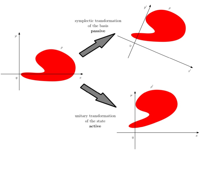
Figure 2.1: Passive and active transformations

When comparing $\rho_{S\hat{R}}$ to $\rho_{\hat{R}}$ in Eq. (2.28) we see that the above transformation could also be done by transforming the state (active) while leaving the basis unchanged. In other words to every symplectic matrix $S\in Sp(2N,\mathbbm{R})$ exists a unitary operator $U(S)$ so, that $\rho_{\hat{R}}\mapsto\rho_{S\hat{R}}=U^{{\dagger}}(S)~{}\rho_{\hat{R}}~{}U(S)$.

2.6 Bipartite Entanglement

The crucial feature quantum mechanics provides for quantum information theory is entanglement. It is a purely quantum phenomenon with a lot of counterintuitive consequences. When measuring different parts of a composite system ($\mathcal{H}=\mathcal{H}_{A}\otimes\mathcal{H}_{B}$) the outcomes of the measurements may be correlated. This correlation could be generated by a preparation of the state using only operations on each part of the system (local), classical communication and statistical mixing (LOCC). States which could be prepared like this will be called classically correlated or separable. But this is not the whole story. In quantum theory a stronger kind of correlations can be observed. The so called entangled states are non-local in the sense that they can not be prepared by LOCC and that both parts of an entangled pair do not have their own properties but contain only joint information.

The definition of separability shows the tensor product structure of locally produced states plus mixing.

Definition 2.6 (Separability)

A state $\rho$ is separable with respect to the split $A|B$ iff it can be written (or approximated, e.g., in trace norm), with probabilities $p_{i}\geq 0$ and $\sum_{i}p_{i}=1$ and proper density matrices $\rho_{i}^{(A)}$ and $\rho_{i}^{(B)}$ belonging to the parties $A$ and $B$ respectively, as

$$\rho=\sum_{i}p_{i}\,\rho_{i}^{(A)}\otimes\rho_{i}^{(B)}$$ (2.29)

that is, the closed convex hull of product states. Otherwise the state is called entangled. The set of separable density matrices $\rho$ on $\mathcal{H}_{A}\otimes\mathcal{H}_{B}$ ( with respect to the split $A|B$) will be denoted by $S_{{A|B}}(\mathcal{H})$ and is a closed convex subset of $S(\mathcal{H})$ defined in Def. 2.2.

We see that this definition gives rise to complications since it is not easy to find out whether a given state $\rho$ can be written in the form (2.29) or not. A significant amount of research has been done to find simpler criteria to decide whether a given state is entangled or not. One of the most famous criteria is the so called PPT-criterion.

Theorem 2.2 (PPT criterion for bipartite systems)

Let $\rho$ be a state on a Hilbert space $\mathcal{H}=\mathcal{H}_{A}\otimes\mathcal{H}_{B}$ which has a non-positive partial transpose then the state is entangled with respect to the split $A|B$.

$$\rho^{T_{A}}\not\geq 0\Rightarrow\rho\mbox{ is entangled}$$

In the cases $1.\,\mathcal{H}_{A}=\mathcal{H}_{B}=\mathbbm{C}^{2}$, $2.\,\mathcal{H}_{A}=\mathbbm{C}^{2}$ and $\mathcal{H}_{B}=\mathbbm{C}^{3}$ and $3.$ for Gaussian states split into $1_{A}\times N_{B}$ modes this criterion is also sufficient.

The necessary direction for entanglement was formulated by A. Peres in 1996 Ref. [14]. The sufficiency was shown by M.+ P.+R. Horodecki ($1$ and $2$) in 1996 Ref. [15] and R.F. Werner and M.M. Wolf ($3$) in 2000 Ref. [16]. The name PPT criterion is an abbreviation of positive partial transpose.

The partial (say $A$) transpose of a state is the state transposed only on one of its subsystems (only $A$). In formulae: $\rho_{\alpha,n;\beta,m}=(\rho^{T_{A}})_{\beta,n;\alpha,m}$ where $\alpha,\beta$ and $n,m$ belong to the parties $A$ and $B$ respectively. Note, that $\rho^{T_{A}}$ is still selfadjoint and has trace one. The partial transpose of a state is only a mathematical tool and cannot perfectly be performed by a physical transformation. Sometimes the partial transpose of a system’s state is understood as a time reversal in the transposed part only. Phase conjugation in laser beams actually realise such a time reversal but it can not be done perfectly since there always comes a small amount of noise with it (see Example 7 in the fourth chapter for a little discussion).

Almost every application in QIT uses non-classical correlations, e.g., teleportation [17, 18, 19], quantum cryptography [20, 21, 22] and dense coding [23]. Because all these funny things strongly depend on the entanglement of the used states it is often understood as a resource. Naturally one wants to know how much of that resource one has. Due to its importance a great deal of effort has been invested in the last decade, to find a sensible measure quantifying entanglement. Several entanglement measures have been proposed, for example the entanglement of formation in Ref. [24, 25] and the distillable entanglement in Ref. [26] and further discussions in Ref. [27, 28]. We introduce two quantities strongly related to entanglement measures, which we will need later on. The von Neumann entropy is the the quantum analogue of the Shannon entropy Ref. [29] and gives the degree of mixedness or impurity of a state.

Definition 2.7 (von Neumann entropy)

The von Neumann entropy of a mixed state $\rho\in S(\mathcal{H})$ is defined as

$$S(\rho):=-tr[\rho\,\ln\rho]=-\sum_{i}\,p_{i}\ln p_{i}$$

where the $p_{i}$ are the eigenvalues of the state $\rho$.

The only so far computable entanglement measure is the logarithmic negativity, Ref. [30, 31, 32, 33]. With $||A||_{1}:=tr[\sqrt{A^{{\dagger}}A}]$ we define the logarithmic negativity

Definition 2.8

The logarithmic negativity of a bipartite state $\rho\in$ is given by

$$E_{\mathcal{N}}(\rho):=\ln||\rho^{T_{A}}||_{1}.$$

with respect to the split $A|B$.

If $\rho^{T_{A}}$ has negative eigenvalues $\lambda_{i}(\rho^{T_{A}})$ fulfilling $1=tr[\rho^{T_{A}}]=\sum_{i}\lambda_{i}(\rho^{T_{A}})$, the sum of the absolute values of the eigenvalues must be greater than one: $||\rho^{T_{A}}||_{1}=\sum_{i}|\lambda_{i}(\rho^{T_{A}})|>1$. Hence the logarithmic negativity of $\rho$ is greater than $0$. If $\rho$ has a positive partial transpose $\rho^{T_{A}}\geq 0$, the logarithmic negativity vanishes since $tr[\sqrt{\rho^{T_{A}}\rho^{T_{A}}}]=tr[\rho^{T_{A}}]=1$. For all separable states this is true. But there may also exist entangled states with PPT unless the PPT-criterion is also sufficient. In this thesis we will mainly discuss the case where the PPT-criterion is also sufficient, namely for Gaussian states of $1_{A}\times N_{B}$ modes. Note, that for all elements of $S(\mathcal{H})$ the logarithmic negativity is positive definite.

Chapter 3 Gaussian States

In quantum information theory more and more attention is paid to continuous variable states. Gaussian states are a nice target to exploit since they are available not only theoretically but can be observed and prepared in the lab. For example, any laser produces Gaussian states and most optical setup laser light can go through preserves this property. From the mathematical point of view they are the simplest case of nontrivial CVS showing squeezing and entanglement. To learn how one can use continuous variable states for QIT purposes Gaussian states play the key role and will be characterised in this chapter.

Definition 3.1

A Gaussian $N-$mode state $\rho$ is a state, whose characteristic function defined in Def. 2.5 can be written as:

$$\chi_{\rho}(\xi)=\exp[-{1\over 4}\xi^{T}\Gamma\xi+i\vec{D}^{T}\xi],\qquad\xi\in\mathbbm{R}^{2N},$$ (3.1)

where $\Gamma$ is the covariance matrix of the state and $\vec{D}$ the displacement vector.

No other parameters appear since in analogy to classical probability distributions the quantum Gaussian states are determined by their first and second moments alone. When describing Gaussian states, we will often use only their covariance matrices since they reflect all important properties Gaussian states can have. We will investigate those properties in the subsequent sections after introducing some examples of Gaussian states.

Unfortunately in the literature both, the matrix $\gamma$ defined in Eq. (2.3) and the matrix $\Gamma$ appearing in the characteristic function above, are called covariance matrix. Usually it is clear which one is meant and therefore we will not distinguish them explicitly. As a general rule in mathematical formulae we will use small greek letters in the first case and capital letters in the second. The same holds for the displacements $\vec{d}$ and $\vec{D}$. The two displacement vectors and the two matrices can be transformed into each other using the symplectic matrix defined in Eq. (2.2) with the following transformation law:

$$\vec{D} = \sigma\,\vec{d}\,\mbox{ and }\,\Gamma=\sigma\,\gamma\,\sigma^{T}.$$ (3.2)

As one can easily check the $\Gamma$-matrix again fulfills covariance matrix properties.

3.1 Coherent, Squeezed and Thermal States

We introduce three important classes of pure one mode Gaussian states, namely the coherent, the squeezed and the thermal states of an electromagnetic field mode. General reference for this section is Ref. [10] by S.M. Barnett and P.M. Radmore.

Coherent States

The coherent states are defined as the eigenvectors of the non hermitian annihilation operator $\hat{a}$ : $\hat{a}|\alpha\rangle=\alpha|\alpha\rangle,$ with $\alpha$ being a complex eigenvalue, and one easily finds that those state vectors are superpositions of number state vectors of the form

$$|\alpha\rangle=e^{-{|\alpha|^{2}\over 2}}\,\sum_{n=0}^{\infty}\,{\alpha^{n}\over\sqrt{n!}}\,|n\rangle.$$ (3.3)

They can be generated from the vacuum with the unitary operators $\hat{D}(\alpha)$ introduced in Eq. (2.26) which induce displacements in phase space.

$$\hat{D}(\alpha) = e^{\alpha\hat{a}^{{\dagger}}-\alpha^{*}\hat{a}}=e^{\alpha\hat{a}^{{\dagger}}}e^{-\alpha^{*}\hat{a}}e^{-{|\alpha|^{2}\over 2}},$$

$$|\alpha\rangle := \hat{D}(\alpha)|0\rangle.$$

They are an overcomplete nonorthogonal set of state vectors spanning the entire Hilbert space resolving unity,

$$\hat{\mathbbm{1}}=\int{\mbox{\rm{d}}\Re(\alpha)\mbox{\rm{d}}\Im(\alpha)\over\pi}|\alpha\rangle\langle\alpha|,$$

and the scalar product between two coherent states

$$\langle\alpha|\beta\rangle=e^{-{|\alpha|^{2}+|\beta|^{2}-2\alpha^{*}\beta\over 2}}.$$

With $\alpha={\eta_{1}+i\eta_{2}\over\sqrt{2}}$ and the identification Eq. (2.26) we calculate the characteristic function of the coherent states:

$$\chi_{\alpha}(\xi) = tr[|\alpha\rangle\langle\alpha|\hat{W}_{\xi}]=tr[\hat{D}(\alpha)|0\rangle\langle 0|\hat{D}(-\alpha)\hat{W}_{\xi}]$$

$$= tr[\hat{W}_{-\eta}|0\rangle\langle 0|\hat{W}_{\eta}\hat{W}_{\xi}]=e^{-{i\over 2}\eta^{T}\sigma\xi}\,\langle 0|\hat{W}_{\eta+\xi}\hat{W}_{-\eta}|0\rangle$$

$$= e^{-{i\over 2}\eta^{T}\sigma\xi}\,e^{{i\over 2}(\eta+\xi)^{T}\sigma\eta}\,\langle 0|\hat{W}_{\xi}|0\rangle=e^{-{\xi_{1}^{2}+\xi_{2}^{2}\over 4}}\,e^{-{i}\eta^{T}\sigma\xi}$$

$$= e^{-{\xi_{1}^{2}+\xi_{2}^{2}\over 4}}\,e^{-{i}\sqrt{2}(\Re(\alpha),\Im(\alpha))\sigma\xi},$$

where we used the cyclicity of the trace, the Weyl relations from Lemma 2.3 and $\langle 0|\hat{W}_{\xi}|0\rangle=e^{-{\xi_{1}^{2}+\xi_{2}^{2}\over 4}}$.

The coherent states are thus of Gaussian type and furthermore all of them have the same covariance matrix: $\Gamma_{\alpha}=\mathbbm{1}$, while the displacements depend on the value of $\alpha$: $\vec{D}_{\alpha}=\sqrt{2}\left(\begin{array}[]{c}\Im\,(\alpha)\\ -\Re\,(\alpha)\end{array}\right).$ Similarly, we have $\gamma_{\alpha}=\sigma\Gamma_{\alpha}\sigma^{T}=\mathbbm{1}$ and $\vec{d}_{\alpha}=-\sigma\vec{D}_{\alpha}=\sqrt{2}\left(\begin{array}[]{c}\Re\,(\alpha)\\ \Im\,(\alpha)\end{array}\right)$. The uncertainty relation is exactly fulfilled with $\Delta^{2}\hat{x}\cdot\Delta^{2}\hat{p}={1\over 4}$ and is equally stretched in all directions in phase space. Therefore coherent states can be pictured as circles of diameter ${1\over\sqrt{2}}$ around the points $(\sqrt{2}\Re(\alpha),\sqrt{2}\Im(\alpha))$. For $\alpha=0$ the coherent state vector $|0\rangle$ is just the vacuum with $\Gamma_{0}=\gamma_{0}=\mathbbm{1}$ and $\vec{D}_{0}=\vec{d}_{0}=0$.

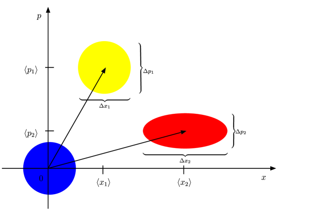
Figure 3.1: States in phase space

The picture shows the vacuum state (blue), a coherent state (yellow) and a displaced squeezed vacuum (red). They all span the same area meaning that the product $\Delta^{2}x\cdot\Delta^{2}p$ is the same for all states, namely it is ${1\over 4}$, the lower bound of the uncertainty relation. Hence all these states are minimal uncertainty states.

Squeezed States

Similarly one can produce states with non-energy conserving squeezing operators $\hat{S}(\zeta)$, though experimentally it is difficult to realise such a transformation requiring strong Kerr media.

$$\hat{S}(\zeta) := e^{-{\zeta\over 2}\hat{a}^{2{\dagger}}+{\zeta^{*}\over 2}\hat{a}^{2}}$$

$$= e^{-{1\over 2}\exp[i\phi]\tanh r\,\hat{a}^{2{\dagger}}}\,e^{-{1\over 2}\ln(\cosh r)(\hat{a}^{{\dagger}}\hat{a}+\hat{a}\hat{a}^{{\dagger}})}\,e^{{1\over 2}\exp[-i\phi]\tanh r\,\hat{a}^{2}}.$$

$\hat{S}$ is unitary since it is $\hat{S}(\zeta)=\hat{S}^{{\dagger}}(-\zeta)$ with $\zeta=re^{i\phi}$. The squeezed vacuum is prepared by letting a squeezing operator act on the vacuum.

$$|\zeta\rangle := \hat{S}(\zeta)|0\rangle$$

$$= {1\over\sqrt{\cosh r}}\sum_{n=0}^{\infty}{\sqrt{(2n)!}\over n!}\,(-{1\over 2}\exp[i\phi]\tanh r)^{n}\,|2n\rangle.$$

The characteristic function of the squeezed vacuum with $\alpha={\xi_{1}+i\xi_{2}\over\sqrt{2}}$ is:

$$\chi_{\zeta}(\xi) = tr[|\zeta\rangle\langle\zeta|\hat{W}_{\xi}]$$

$$= \langle 0|\hat{S}(-\zeta)\hat{D}(-\alpha)\hat{S}(\zeta)|0\rangle$$

$$= \langle 0|\hat{S}(-\zeta)\hat{S}(\zeta)\hat{D}(-\alpha^{\prime})|0\rangle=e^{-{|\alpha|^{2}\over 2}}$$

with $\alpha^{\prime}$ determined by commutator of $\hat{D}(-\alpha)$ with $\hat{S}(\zeta)$ and given by

$$\alpha^{\prime} = {\xi_{1}[\cosh r+\cos\phi\sinh r]+\xi_{2}\sin\phi\sinh r\over\sqrt{2}}$$

$$+ i\,{\xi_{1}\sin\phi\sinh r+\xi_{2}[\cosh r-\cos\phi\sinh r]\over\sqrt{2}}$$

we get

$$\chi_{\zeta}(\xi) = e^{-{1\over 4}\xi_{1}^{2}(\cosh 2r+\sinh 2r\cos\phi)}\,e^{-{1\over 4}\xi_{2}^{2}(\cosh 2r-\sinh 2r\cos\phi)}$$

$$\times\,e^{-{1\over 2}\xi_{1}\xi_{2}\sinh 2r\sin\phi},$$

and hence all squeezed vacua are of Gaussian type. They have vanishing displacements and covariance matrices

$$\Gamma_{\zeta}=\left(\begin{array}[]{cc}\cosh 2r+\sinh 2r\cos\phi&\sinh 2r\sin\phi\\ \sinh 2r\sin\phi&\cosh 2r-\sinh 2r\cos\phi\end{array}\right).$$

From the CM one can read off that the variance of the state in one direction of the phase space is different than in the other; that is why the states are called squeezed. But the uncertainty relation is still fulfilled as a short check shows.

$$\Delta^{2}\hat{x}\cdot\Delta^{2}\hat{p} = {1\over 4}(\cosh 2r+\sinh 2r\cos\phi)(\cosh 2r-\sinh 2r\cos\phi)$$

$$= {1\over 4}(\cosh^{2}2r-\sinh^{2}2r\cos\phi)={1\over 4}+{\sinh^{2}2r\sin^{2}\phi\over 4}\geq{1\over 4},$$

where equality (minimal uncertainty) is reached for $r=0$ or $\phi=0$. In the first case there is no squeezing at all, $\hat{S}(0)=\mathbbm{1}$, and we again have the vacuum. In the second case $\Gamma_{\zeta}$ has the form

$$\Gamma_{\zeta=r}=\left(\begin{array}[]{cc}\cosh 2r+\sinh 2r&0\\ 0&\cosh 2r-\sinh 2r\end{array}\right)=\left(\begin{array}[]{cc}e^{2r}&0\\ 0&e^{-2r}\end{array}\right),$$

where we recognise that $\Gamma_{\zeta=r}$ could be prepared from the vacuum with the symplectic squeezing transformation introduced in Example 2 of the second chapter with the squeezing parameter $d=e^{r}$. All squeezed states can be prepared from the vacuum by a squeezing operation (squeezed vacuum) and an additional displacement in phase space.

Thermal States

The statistical concept of equilibrium states or Gibbs states is naturally taken to the quantum world. We define the thermal state of a system described by a Hamiltonian $\hat{H}$ as the exponential of the Hamiltonian together with the factor $\beta={1\over k_{B}T},$ where $k_{B}$ is the Boltzmann constant and $T$ is the temperature of the system. For a one mode harmonic oscillator the well known Hamiltonian is given by $\hat{H}=\omega(\hat{n}+{1\over 2})$, with $\hat{n}=\hat{a}^{{\dagger}}\hat{a}$ being the number operator of the mode and $\hbar=1$ throughout this thesis. The thermal state for this Hamiltonian is given by

$$\rho_{t} = {e^{-\beta\hat{H}}\over tr[e^{-\beta\hat{H}}]}$$

$$= \sum_{n,m}|n\rangle\langle n|{e^{-\beta\omega(\hat{n}+{1\over 2})}\over tr[e^{-\beta\omega(\hat{n}+{1\over 2})}]}|m\rangle\langle m|$$

$$= {1\over tr[e^{-\beta\omega(\hat{n}+{1\over 2})}]}\sum_{n}e^{-\beta\omega(n+{1\over 2})}|n\rangle\langle n|,$$

with $tr[e^{-\beta\omega(\hat{n}+{1\over 2})}]={1\over 2\sinh{\beta\omega\over 2}}$.

The characteristic function then is:

$$\chi_{t}(\xi) = 2\,\sinh{\beta\omega\over 2}\,\,\,tr\left[\sum_{n}|n\rangle\langle n|e^{-\beta\omega(n+{1\over 2})}\hat{W}_{\xi}\right]$$

$$\chi_{t}(\xi) = 2\,\sinh{\beta\omega\over 2}\,\,\,\sum_{n}e^{-\beta\omega(n+{1\over 2})}\langle n|\hat{W}_{\xi}|n\rangle.$$

The elements of the Weyl operators in the number basis with $\alpha={\xi_{1}+i\xi_{2}\over\sqrt{2}}$ are

$$\langle n|\hat{W}_{\xi}|m\rangle = \langle n|\hat{D}(-\alpha)|m\rangle=\langle 0|{\hat{a}^{n}\over\sqrt{n!}}\hat{D}(-\alpha){\hat{a}^{{\dagger}\,m}\over\sqrt{m!}}|0\rangle$$

$$= {\begin{cases}e^{-{|\alpha|^{2}\over 2}}(-\alpha)^{n-m}\sqrt{m!n!}\sum_{l=0}^{m}{(-|\alpha|^{2})^{l}\over l!(m-l)!(l+n-m)!}&\,m\leq n\\ e^{-{|\alpha|^{2}\over 2}}(\alpha^{*})^{m-n}\sqrt{m!n!}\sum_{l=0}^{n}{(-|\alpha|^{2})^{l}\over l!(n-l)!(l+m-n)!}&\,m\geq n\end{cases}}$$

$$= {\begin{cases}e^{-{|\alpha|^{2}\over 2}}(-\alpha)^{n-m}\sqrt{{m!\over n!}}L_{m}^{n-m}(|\alpha|^{2})&\,m\leq n\\ e^{-{|\alpha|^{2}\over 2}}(\alpha^{*})^{m-n}\sqrt{{n!\over m!}}L_{n}^{m-n}(|\alpha|^{2})&\,m\geq n,\\ \end{cases}}$$

where $L_{n}^{k}(x)$ are the Laguerre polynomials; so we get for $n=m$ :

$$\langle n|\hat{W}_{\xi}|n\rangle = \langle n|\hat{D}(-\alpha)|n\rangle=e^{-{|\alpha|^{2}\over 2}}L_{n}^{0}(|\alpha|^{2}),$$

and $\chi_{t}$ becomes

$$\chi_{t}(\xi) = 2\sinh{\beta\omega\over 2}e^{-{|\alpha|^{2}\over 2}}\sum_{n}e^{-\beta\omega(n+{1\over 2})}L_{n}^{0}(|\alpha|^{2}).$$

With sum formula (8.975.1) in Ref. [34] we finally get

$$\chi_{t}(\xi) = 2\sinh{\beta\omega\over 2}e^{-{|\alpha|^{2}\over 2}}e^{-{\beta\omega\over 2}}{1\over 1-e^{-\beta\omega}}{e^{|\alpha|^{2}e^{-\beta\omega}\over e^{-\beta\omega}-1}}$$

$$= e^{-{|\alpha|^{2}\over 2}}e^{-|\alpha|^{2}\over e^{\beta\omega}-1}=e^{-{\xi_{1}^{2}+\xi_{2}^{2}\over 4}{e^{\beta\omega}+1\over e^{\beta\omega}-1}}$$

$$= e^{-{\xi_{1}^{2}+\xi_{2}^{2}\over 4\tanh{\beta\omega\over 2}}}.$$

Hence the thermal state is a Gaussian state with vanishing displacement and covariance matrix

$$\Gamma_{t}={1\over\tanh{\beta\omega\over 2}}\mathbbm{1}=\gamma_{t},$$ (3.4)

that is, a diagonal $2\times 2$ matrix with identical entries. We will meet the thermal states again when discussing normal forms of CMs in the next chapter. In the limit $\beta={1\over k_{B}T}\to\infty$ we get $\tanh{\beta\omega\over 2}\to 1$ and hence

$$\chi_{(T=0)}(\xi)=e^{-{\xi_{1}^{2}+\xi_{2}^{2}\over 4}},$$

that is, the thermal state becomes the vacuum in the limit of zero temperature.

3.2 Normal Forms of Covariance Matrices

Covariance matrices are real symmetric matrices, hence it is always possible to diagonalise a CM with orthogonal matrices to the standard normal form which is the diagonal matrix of the eigenvalues of the CM. But other, symplectic, normal forms exist which are more convenient for covariance matrices because the resulting quantities are invariant under subgroups of the symplectic transformations. We introduce two very important normal forms which are used extensively in the following chapters.

3.2.1 Williamson Normal Form

Surprisingly it is possible to diagonalise real positive symmetric and even-dimensional matrices with symplectic matrices. The resulting diagonal matrix is called Williamson normal form and the proof of existence and uniqueness was given by J.Williamson in 1936, see Ref. [35].

Theorem 3.1 (Williamson normal form)

For every real strictly positive symmetric $2N\times 2N$ matrix $A$ there exists a matrix $S\in Sp(2N,\mathbbm{R})$, so that

$$A^{WNF}=SAS^{T}=\left(\begin{array}[]{ccccc}a_{1}&0&&0&0\\ 0&a_{1}&&0&0\\ &&\ddots&&\\ 0&0&&a_{N}&0\\ 0&0&&0&a_{N}\end{array}\right)$$ (3.5)

with the symplectic eigenvalues $a_{i}>0$ for all $i=1,\ldots,N$. The symplectic matrix $S$ and the diagonal entries $a_{i}$ are unique up to permutations of the diagonal entries in $A^{WNF}$.

Remark: If $A$ had a vanishing eigenvalue it would not be possible to bring it to the above form. Instead, Williamson-diagonalise the regular, positive principal submatrices of the matrix $A$. Now transform the singular submatrix $A_{0}$ of $A$ to its orthogonal diagonal form $D_{0}=O^{T}A_{0}O=\left(\begin{array}[]{cc}0&0\\ 0&a_{0}\end{array}\right)$ with $O\in SO(2,\mathbbm{R})\subset Sp(2,\mathbbm{R})$. The symplectic eigenvalue of $A_{0}$ is counted as zero.

Note, that the determinant of $A$ is easily calculated from its symplectic eigenvalues: $\det A=\prod_{i=1}^{N}a_{i}^{2}$ and that the symplectic eigenvalues of a matrix are invariant under symplectic transformations.

Especially covariance matrices can be Williamson-diagonalised and as we will see in the following discussion of the Williamson normal form the transformed covariance matrix $\Gamma^{WNF}=\bigoplus_{i=1}^{N}s_{i}\mathbbm{1}_{2\times 2}$ describes the state of N uncoupled harmonic oscillators in a heat bath with temperatures $T_{i}=T_{i}(s_{i})$.

Symplectic Eigenvalues

In general it is difficult to find the symplectic transformation which brings a given matrix to Williamson normal form, but the eigenvalues are easily calculated with the following lemma

Lemma 3.1

The symplectic eigenvalues of a real symmetric positive $2N\times 2N$ matrix $A$ are the positive eigenvalues of the matrix $i\sigma A$.

Proof : With $A=S^{-1}A^{WNF}S^{-T}$

$$\mbox{spec}(i\sigma A) = \mbox{spec}(i\sigma S^{-1}A^{WNF}S^{-T})=\mbox{spec}(iS^{T}\sigma A^{WNF}S^{-T})$$

$$= \mbox{spec}(iS^{-T}S^{T}\sigma A^{WNF})=\mbox{spec}(i\sigma A^{WNF})$$

$$= \mbox{spec}\left(i\bigoplus_{j=1}^{N}\left[a_{j}\left(\begin{array}[]{cc}0&1\\ -1&0\end{array}\right)\right]\right)$$

were we used the properties of symplectic matrices and the cyclicity of the spectrum, see Lemma A.4. The eigenvalues $\lambda_{i}$ of $i\sigma A^{WNF}$ are calculated via

$$0 \overset{!}{=} \det[i\sigma A^{WNF}-\lambda_{i}\mathbbm{1}]=\left|\bigoplus_{j=1}^{N}\left[\begin{array}[]{cc}-\lambda_{i}&ia_{j}\\ -ia_{j}&-\lambda_{i}\end{array}\right]\right|$$

$$= \prod^{N}_{j=1}\left|\begin{array}[]{cc}-\lambda_{i}&ia_{j}\\ -ia_{j}&-\lambda_{i}\end{array}\right|=\prod^{N}_{j=1}(\lambda_{i}^{2}-a_{j}^{2}),$$

we find the spectrum of $i\sigma A$ to be $\mbox{spec}(i\sigma A)=\{a_{i},-a_{i}\}_{i=1}^{N}$ completing the proof of the lemma. $\Box$

Example 6 : Given a covariance matrix $\Gamma=\left(\begin{array}[]{cc}3&1\\ 1&1\end{array}\right)$ then the symplectic eigenvalues of $\Gamma$ are the positive eigenvalues of $i\sigma\Gamma=\left(\begin{array}[]{cc}i&i\\ -3i&-i\end{array}\right).$ The eigenvalues are $\lambda_{1,2}=\pm\sqrt{2}$, so the symplectic eigenvalue of $\Gamma$ is $\Gamma_{1}=\sqrt{2}$. Even faster is $\det\Gamma=2=\Gamma_{1}^{2}$, thus $\Gamma_{1}=\sqrt{2}$.

Thermal States

Question: Given a covariance matrix in Williamson normal form and displacement $\vec{D}$, what is the corresponding Gaussian state $\rho$ ?

We first see how block diagonal covariance matrices $\Gamma=\bigoplus_{i=1}^{N}\Gamma_{i}$ are related to product states.

Lemma 3.2 (Block diagonal CMs)

A Gaussian state $\rho$ with a covariance matrix in block diagonal form is a product state, and conversely if $\rho$ is a state of product form then its covariance matrix is of block diagonal form.

Proof : We use the decomposition of $\rho$ in the Weyl system according to Eq. (2.27) and insert the characteristic function with the given block diagonal matrix $\Gamma=\bigoplus_{i=1}^{N}\Gamma_{i}$ and displacement $\vec{D}$. For $\xi\in\mathbbm{R}^{2N}$ and $\xi_{i}\in\mathbbm{R}^{2},\quad\forall i=1,...N$, $\rho$ can be decomposed

$$\rho = {1\over(2\pi)^{N}}\,\int\,\mbox{\rm{d}}^{2N}\xi\;e^{-{\xi^{T}\Gamma\xi\over 4}+i\vec{D}^{T}\xi}\,\hat{W}_{\xi}$$

$$= {1\over(2\pi)}\,\int\,\prod_{i=1}^{N}(\mbox{\rm{d}}^{2}\xi_{i})\;e^{-{\sum_{i=1}^{N}\xi_{i}^{T}\Gamma_{i}\xi_{i}\over 4}}\,e^{i\sum_{i=1}^{N}\vec{D}_{i}^{T}\xi_{i}}\,\bigotimes_{i=1}^{N}\hat{W}_{\xi_{i}}$$

$$= \bigotimes_{i=1}^{N}\left[{1\over(2\pi)}\,\int\,\mbox{\rm{d}}^{2}\xi_{i}\;e^{-{\xi_{i}^{T}\Gamma_{i}\xi_{i}\over 4}+i\vec{D}_{i}^{T}\xi_{i}}\,\hat{W}_{\xi_{i}}\right]$$

$$= \bigotimes_{i=1}^{N}\rho_{i},$$

where the $\rho_{i}$ are one-mode Gaussian states with covariance matrices $\Gamma_{i}$ and displacements $\vec{D}_{i}$. $\Box$

We learned in Section 3.1 that the one-mode thermal states of the harmonic oscillator have the covariance matrix $\Gamma_{t}={1\over\tanh{\beta\omega\over 2}}\mathbbm{1}$ and vanishing displacement. Since there is a one to one correspondence between the pairs $\Gamma$ and $\vec{D}$ and the Gaussian states $\rho$, the displaced thermal states are the only ones having such a diagonal matrix. The Gaussian state belonging to a CM in Williamson normal form $\Gamma=\bigoplus_{i=1}^{N}s_{i}\mathbbm{1}$ with symplectic eigenvalues $s_{i}$ and displacement $\vec{D}$ is a product state of displaced thermal states with independent heat baths of temperature $T_{i}$.

$$\rho=\bigotimes_{i=1}^{N}\rho_{i}=\bigotimes_{i=1}^{N}\hat{W}_{\vec{D}}\,\rho_{t}(T_{i})\,\hat{W}^{{\dagger}}_{\vec{D}}\,.$$

The symplectic eigenvalues of the CM are then connected to the temperature of the heat bath namely

$$s_{i}={1\over\tanh{\omega\over 2k_{B}T_{i}}}.$$

3.2.2 Simon Normal Form

We introduce a normal form, as proposed in Ref. [36], acting only locally on the first and second mode respectively and therefore preserve the entanglement properties of a given state $\rho$.

Theorem 3.2 (Simon normal form)

For every two-mode covariance matrix $\Gamma$ there exist matrices $S_{1}\in Sp(2,\mathbbm{R})$ and $S_{2}\in Sp(2,\mathbbm{R})$ so that:

$$\Gamma^{SNF}=(S_{1}\oplus S_{2})\,\Gamma\,(S_{1}^{T}\oplus S_{2}^{T})=\left(\begin{array}[]{cccc}a&0&c&0\\ 0&a&0&d\\ c&0&b&0\\ 0&d&0&b\end{array}\right).$$

This normal form is unique up to the little subtlety that only the relative sign of $c$ and $d$ is determined.

The transformations $S=S_{1}\oplus S_{2}$ are local transformations acting only on the first and second mode respectively, in particular they do not change the entanglement properties of the covariance matrix they are acting on.

Simon Invariants

The determinants of the submatrices of $\Gamma$ and $\Gamma$ itself are preserved by the diagonalising symplectic transformation and appear as the Simon invariants $a,b,c,d$ with the relations:

$$\begin{array}[]{rclrcl}\Gamma&=&\left(\begin{array}[]{cc}A&C\\ C^{T}&B\end{array}\right)&a&=&\sqrt{\det A},\\ &&&b&=&\sqrt{\det B},\\ \det\Gamma&=&a^{2}b^{2}+c^{2}d^{2}-ab(c^{2}+d^{2})&cd&=&\;\;\,\det C.\end{array}$$ (3.14)

We hence reduce our ten parameter covariance matrix to four real numbers still reflecting the entanglement properties of the original CM.

3.3 Properties of Characteristic Numbers

All derived properties of the covariance matrix $\gamma$ translate identically to the matrix $\Gamma=\sigma\,\gamma\,\sigma^{T}$. Namely $\Gamma$ is a real, symmetric, positive matrix fulfilling the uncertainty relation and has the same determinant, eigenvalues and symplectic eigenvalues as $\gamma$.

Simon Invariants and Symplectic Eigenvalues

In the last section we saw that there exist normal forms respecting the symplectic character of the canonical transformations on covariance matrices. These forms were related to invariant quantities whose properties we will discuss in this section. We will also see that properties of the states like squeezing and entanglement are strongly connected to these numbers. We denote the eigenvalues of a given $N-$mode CM $\Gamma$ by $\lambda_{i},$ for $i=1,...,2N$, the symplectic eigenvalues by $\Gamma_{j}$, for $j=1,...,N$ and the Simon invariants (only for two-mode systems) by $a,b,c,d$.

Assume we have a covariance matrix $\Gamma$ in Simon normal form and we want to know the eigenvalues and the symplectic eigenvalues of $\Gamma^{SNF}$. We find that the eigenvalues of $\Gamma^{SNF}$, expressed with the Simon numbers, are given by

$$\begin{split}\lambda^{SNF}_{1,2}&=\frac{a+b}{2}\pm\frac{1}{2}\sqrt{(a-b)^{2}+4c^{2}},\\ \lambda^{SNF}_{3,4}&=\frac{a+b}{2}\pm\frac{1}{2}\sqrt{(a-b)^{2}+4d^{2}}.\end{split}$$ (3.15)

Remark: These numbers in general are not the eigenvalues of $\Gamma$ since in general the symplectic transformations $S_{1}$ and $S_{2}$ are active transformations (see Section 2.2).

Furthermore, the symplectic eigenvalues of a two mode system with covariance matrix $\Gamma^{SNF}$ can be expressed by the Simon invariants via

$$\Gamma_{1,2}=\frac{1}{\sqrt{2}}\sqrt{a^{2}+b^{2}+2cd\pm\sqrt{(a^{2}+b^{2}+2cd)^{2}-4\det\gamma}}.$$ (3.16)

and are the same as the ones of $\Gamma$ itself.

Positivity

From the positivity of $\Gamma$ it follows that

$$\lambda_{i} \geq 0,\quad i=1,\ldots,2N,$$

$$\Gamma_{i} \geq 0,\quad j=1,\ldots,N,$$ (3.17)

$$a,b\geq 1\, \,c^{2}\leq ab,d^{2}\leq ab.$$ and

Uncertainty Relation

The Heisenberg uncertainty principle formulated in Section 2.3 is also true for the capital matrices $\Gamma$ (see Eq. (3.2) and Lemma 2.1). Since the matrix $\Gamma+i\sigma$ is positive it can be brought to Williamson normal form by symplectic transformations $S$ without changing the symplectic eigenvalues. We have:

$$S\,[\Gamma+i\sigma]\,S^{T}=S\,\Gamma\,S^{T}+i\sigma=\Gamma^{WNF}+i\sigma=\bigoplus_{j=1}^{N}\left(\begin{array}[]{cc}\Gamma_{j}&i\\ -i&\Gamma_{j}\end{array}\right).$$ (3.18)

To get a positive matrix all eigenvalues $\mu_{i}$, $i=1,...,2N$, of the above matrix have to be positive. The equations determining these eigenvalues are

$$\prod_{j=1}^{N}\,\,\,[(\Gamma_{j}-\mu_{i})^{2}-1]=0,\quad\mbox{for }i=1,...,2N,$$

and hence

$$\Gamma_{j}\pm 1=\mu_{i}\geq 0,\quad\forall i=1,...,N,\,\forall j=1,...,2N$$

Thus the restrictions on the symplectic eigenvalues of $\Gamma$ are

$$\Gamma_{j}\geq 1,\quad\mbox{ for all }j=1,\ldots,N.$$ (3.19)

Note, that the determinant of $\Gamma$ is therefore always greater than or equal to one. For the Simon invariants we find the following, only necessary, criterion

$$\det\Gamma\geq\det A+\det B+2\det C+1,$$ (3.20)

where $A,B,C$ are the submatrices of $\Gamma$ connected to the Simon invariants via Eq. (3.14)

Pure States

Definition 3.2

A state $\rho$ is called pure iff it can be written as a projector $\rho=|\psi\rangle\langle\psi|$ whereas a mixed state is a convex combinations $\rho=\sum_{i}p_{i}|\psi_{i}\rangle\langle\psi_{i}|$ of the states $|\psi_{i}\rangle\langle\psi_{i}|$ with probabilities $p_{i}$   ($p_{i}\geq 0,\,\,\sum_{i}p_{i}=1$) and at least two $i$ so that $p_{i}>0$.

It is well known that a state $\rho$ is pure iff $tr[\rho^{2}]=1$, but how can one express purity in covariance matrix language?

Lemma 3.3

A Gaussian state $\rho$ with CM $\Gamma$ is pure if and only if

$$\det\Gamma=1\iff\forall i:\Gamma_{i}=1\iff(i\sigma\Gamma)^{2}=\mathbbm{1},$$

where the $\Gamma_{i}$ are the symplectic eigenvalues of $\Gamma$. In the two-mode case the conditions on the Simon invariants are

$$a=b=\cosh r\,\mbox{ and }\,c=-d=\sinh r,$$

where $r$ is a squeezing parameter of the CM.

Proof : We expand the state in the Weyl operator basis and calculate the trace of its square

$$\rho = {1\over(2\pi)^{N}}\int\mbox{\rm{d}}^{2N}\xi\;\chi_{\rho}(-\xi)\,\hat{W}_{\xi}$$

$$tr[\rho^{2}] = {1\over(2\pi)^{2N}}\int\mbox{\rm{d}}^{2N}\xi\int\mbox{\rm{d}}^{2N}\eta\;\chi_{\rho}(-\xi)\,\chi_{\rho}(-\eta)\,tr[\hat{W}_{\xi}\,\hat{W}_{\eta}]$$

$$= {1\over(2\pi)^{N}}\int\mbox{\rm{d}}^{2N}\xi\int\mbox{\rm{d}}^{2N}\eta\;\chi_{\rho}(-\xi)\,\chi_{\rho}(-\eta)\,\delta^{2N}(\xi+\eta)$$

$$= {1\over(2\pi)^{N}}\int\mbox{\rm{d}}^{2N}\xi\;\chi_{\rho}(-\xi)\,\chi_{\rho}(\xi).$$

With $\rho$ being a Gaussian state with covariance matrix $\Gamma$ and arbitrary displacement we get

$$tr[\rho^{2}] = {1\over(2\pi)^{N}}\int\mbox{\rm{d}}^{2N}\xi\;e^{-{\xi^{T}\Gamma\xi\over 2}}={1\over\sqrt{\det\Gamma}}.$$

Hence $\rho$ is pure iff $\det\Gamma=1$. It follows directly that the symplectic eigenvalues $\Gamma_{i}$, all necessarily greater than or equal to one, just take their lower bound. Furthermore half of the eigenvalues of $i\sigma\Gamma$ are one while the others are minus one. Hence $(i\sigma\Gamma)^{2}$ has all eigenvalues equal to one and is the identity matrix. For the Simon invariants we easily get the above relations by inserting the $\Gamma_{i}$ in Eq. (3.16). $\Box$

Squeezed States

If a (general) CV state has a smaller covariance in one direction of the phase space than in another it is said to be squeezed. For a basis independent formulation one has to consider all those symplectic transformations which do not change the degree of squeezing. We encountered those transformations when discussing normal forms of symplectic matrices in Eq. (2.12), where we learned that they are in the intersection of the symplectic and the special orthogonal group.

Definition 3.3

An $N-$mode state $\rho$ with covariance matrix $\Gamma$ is squeezed if and only if

$$\exists\,S\in K(N),\;\exists k:\,(S\,\Gamma\,S^{T})_{kk}<1.$$

Here $K(N)=Sp(2N,\mathbbm{R})\cap SO(2N,\mathbbm{R})$ are the passive symplectic transformations.

We picked only those states which have a smaller covariance in at least one phase space direction than the vacuum state. Unfortunately, the criterion is not practicable, but it can be formulated in terms of the eigenvalues of the CM as the following lemma shows:

Lemma 3.4

An $N-$mode state $\rho$ is squeezed if and only if the smallest eigenvalue $\lambda_{min}$ of the state’s covariance matrix is smaller than one.

Proof : First we show that the diagonal entries of a symmetric matrix $A\in\mbox{Mat}(N\times N,\mathbbm{R})$ are always bigger or equal than the smallest eigenvalue $a_{min}$ of the matrix. Let $\{a_{k}\}_{k=1}^{N}$ be the orthonormal system of eigenvectors of $A$ and $\{e_{j}\}_{j=1}^{N}$ an arbitrary orthonormal basis in $\mathbbm{R}^{N}$, then the diagonal entries of $A$ in that basis are $A_{ii}=\langle e_{i}|A|e_{i}\rangle=\sum_{k,l=1}^{N}\,\langle e_{i}|a_{k}\rangle\langle a_{k}|A|a_{l}\rangle\langle a_{l}|e_{i}\rangle=\sum_{l=1}^{N}\,a_{l}|\langle a_{l}|e_{i}\rangle|^{2}\geq a_{min}\,\sum_{l=1}^{N}\,|\langle a_{l}|e_{i}\rangle|^{2}=a_{min},$ as stated. The passive transformations in $K(N)$ do not change the eigenvalues of the CM and since all diagonal entries are bigger or equal to the smallest eigenvalue we have $\forall\,S\in K(N),\;\forall k:\,(S\,\gamma\,S^{T})_{kk}\geq\lambda_{min}$ with equality when $S$ diagonalises $\Gamma$ to its orthogonal normal form and the $k-$th entry is $\lambda_{min}$. Hence the state can only be squeezed if and only if the smallest eigenvalue of the CM is smaller than one. $\Box$

Entangled States

In Section 2.6 we defined what entanglement is and how one can decide whether a given state $\rho$ is entangled or not. We introduced the partial transpose of a bipartite system and stated the PPT criterion for states $\rho\in S(\mathcal{H})$. For Gaussian states it is possible to formulate this criterion on covariance matrix level. We first see what effect the partial transposition of a state has on the states covariance matrix.

Lemma 3.5

The partially transposed covariance matrix (on part $A$) of a bipartite state $\rho$ of $N=N_{A}+N_{B}$ modes with covariance matrix $\Gamma$ is defined by the state $\rho^{T_{A}}$ with the covariance matrix $\Gamma^{T_{A}}$, which is given by

$$\Gamma^{T_{A}}=(-M_{A}\oplus\mathbbm{1}_{B})\,\Gamma\,(-M_{A}\oplus\mathbbm{1}_{B}),$$ (3.21)

with $M_{A}=M_{A}^{T}=\bigoplus_{i=1}^{N_{A}}\left(\begin{array}[]{cc}1&0\\ 0&-1\end{array}\right)$.

Proof : Partial transposition is a basis dependent non-unitary operation and since it is not a completely positive map, it can not be realised perfectly by physical means. Mathematically the transformation can be done, since the spectrum of the partial transpose is not basis dependent, but we have to choose a basis for the calculation. We denote the (multimode) number basis vectors by $|n_{A}\rangle$ and $|n_{B}\rangle$ for $\mathcal{H}_{A}$ and $\mathcal{H}_{B}$ respectively and calculate the characteristic function of the passively transformed state $\rho\mapsto\rho^{T_{A}}$:

$$\chi_{\rho}(\xi) = tr[\rho\,\hat{W}_{\hat{R},\xi}]=\sum_{n_{A},n_{B}}\langle n_{A}n_{B}|\rho\hat{W}_{\hat{R},\xi}|n_{A}n_{B}\rangle$$

$$= \sum_{n_{A},n_{B},m_{A},m_{B}}\langle n_{A}n_{B}|\rho|m_{A}m_{B}\rangle\langle m_{A}|\hat{W}_{\hat{R}_{A},\xi_{A}}|n_{A}\rangle\langle m_{B}|\hat{W}_{\hat{R}_{B},\xi_{B}}|n_{B}\rangle$$

$$\overset{!}{=} \sum_{m_{A},n_{B},n_{A},m_{B}}\langle n_{A}n_{B}|\,\rho\,|m_{A}m_{B}\rangle\langle n_{A}|\hat{W}_{\hat{R}^{\prime}_{A},\xi_{A}}|m_{A}\rangle\langle m_{B}|\hat{W}_{\hat{R}^{\prime}_{B},\xi_{B}}|n_{B}\rangle$$

$$= tr[\rho^{T_{A}}\,\hat{W}_{\hat{R}^{\prime},\xi}].$$

To determine the passive transformation on the basis operators $\hat{R}$, bringing $\rho$ to $\rho^{T_{A}}$, the above expressions shall be equal. We assume that on system $B$ no changes take place, $\hat{R}_{B}=\hat{R}^{\prime}_{B}$, while for system $A$ a linear homogenous transformation

$$M_{A}=\bigoplus_{i=1}^{N_{A}}M\quad\mbox{ fulfilling }\,\hat{R}^{\prime}_{A}=M_{A}\,\hat{R}_{A}$$

has to be determined. For every single mode $i\in A$ we have by the definition of the Weyl operators:

$$\langle m_{i}|\hat{W}_{\hat{R}_{i},\xi_{i}}|n_{i}\rangle = \langle n_{i}|\hat{W}_{M\hat{R}_{i},\xi_{i}}|m_{i}\rangle=\langle n_{i}|e^{i\xi_{i}^{T}\sigma M\hat{R}_{i}}|m_{i}\rangle.$$ (3.22)

The $2\times 2$-matrix $M$ is not a symplectic matrix because if it was one, partial transposition could in principle be realised perfectly. Additionally from symmetry considerations $M$ has to be selfinverse so that the determinant of $M$ has to be minus one. Therefore it fulfills $M\sigma M^{T}=-\sigma$ and expression (3.22) becomes:

$$\langle n_{i}|e^{i\xi_{i}^{T}\sigma M\hat{R}_{i}}|m_{i}\rangle = \langle n_{i}|e^{-i(M^{-1}\xi_{i})^{T}\sigma\hat{R}_{i}}|m_{i}\rangle$$

$$= \langle n_{i}|\hat{W}_{\hat{R}_{i},-M^{-1}\xi_{i}}|m_{i}\rangle$$

$$= \langle m_{i}|\hat{W}_{\hat{R}_{i},M^{-1}\xi_{i}}|n_{i}\rangle^{*}.$$

With the complex numbers $\alpha_{i}={\xi^{1}_{i}+i\xi^{2}_{i}\over\sqrt{2}}$ and $\beta_{i}=\sum_{j=1}^{2}{M^{-1}_{1j}\xi^{j}_{i}+iM^{-1}_{2j}\xi^{j}_{i}\over\sqrt{2}}$ and with Eq. (3.1) we get :

$$\langle m_{i}|\hat{W}_{\hat{R}_{i},\xi_{i}}|n_{i}\rangle = \langle m_{i}|\hat{D}(-\alpha)|n_{i}\rangle$$

$$= {\begin{cases}e^{-{|\alpha_{i}|^{2}\over 2}}(-\alpha_{i})^{m_{i}-n_{i}}\sqrt{{n_{i}!\over m_{i}!}}L_{n_{i}}^{m_{i}-n_{i}}(|\alpha_{i}|^{2})&\,n_{i}\leq m_{i},\\ e^{-{|\alpha_{i}|^{2}\over 2}}(\alpha^{*}_{i})^{n_{i}-m_{i}}\sqrt{{m_{i}!\over n_{i}!}}L_{m_{i}}^{n_{i}-m_{i}}(|\alpha_{i}|^{2})&\,n_{i}\geq m_{i},\\ \end{cases}}$$

$$\overset{!}{=}$$

$$\langle m_{i}|\hat{W}_{\hat{R},M^{-1}\xi_{i}}|n_{i}\rangle^{*} = {\begin{cases}e^{-{|\beta_{i}|^{2}\over 2}}(-\beta^{*}_{i})^{m_{i}-n_{i}}\sqrt{{n_{i}!\over m_{i}!}}L_{n_{i}}^{m_{i}-n_{i}}(|\beta_{i}|^{2})&\,n_{i}\leq m_{i},\\ e^{-{|\beta_{i}^{2}|\over 2}}(\beta_{i})^{n_{i}-m_{i}}\sqrt{{m_{i}!\over n_{i}!}}L_{m_{i}}^{n_{i}-m_{i}}(|\beta_{i}|^{2})&\,n_{i}\geq m_{i},\end{cases}}$$

hence $\beta_{i}=\alpha^{*}_{i}$ and therefore $M^{-1}=M=\left(\begin{array}[]{cc}1&0\\ 0&-1\end{array}\right)=M^{T}$. On the canonical operators, the displacement and the covariance matrices, this transformation acts according to Eq. (2.7) and Eq. (2.23) (even if the transformation is not symplectic but linear homogeneous):

$$\hat{R}\mapsto\hat{R}^{\prime}\;\; = \left(M_{A}\oplus\mathbbm{1}_{B}\right)\,\hat{R},$$

$$\gamma\mapsto\gamma^{T_{A}} = (M_{A}\oplus\mathbbm{1}_{B})\,\gamma\,(M_{A}\oplus\mathbbm{1}_{B}),$$ (3.23)

$$\Gamma\mapsto\Gamma^{T_{A}} = (-M_{A}\oplus\mathbbm{1}_{B})\,\Gamma\,(-M_{A}\oplus\mathbbm{1}_{B}),$$

since $\sigma M_{A}=-M_{A}\sigma$. $\Box$

Note, that partial transposition leads to a reversal of all momenta in the system $A$ while the positions stay unchanged and the system $B$ is untouched. We finally got a recipe of calculating the partially transposed covariance matrix.

Attention: There is a little inconsistency with the definiton of the partially transposed covariance matrix since one does not transpose one part of the matrix, as one does when calculating the partial transpose of a state. Instead, it is the covariance matrix associated to the partial transpose of the state and is calculated by appling a non-symplectic transformation $T=-M_{A}\oplus\mathbbm{1}_{B}$.

We easily see that $\Gamma^{T_{A}}$ is still a real, symmetric, positive matrix but if the partial transpose of $\rho$ fails to be positive its covariance matrix $\Gamma^{T_{A}}$ by Eq. (2.21) does not fulfil the uncertainty relation anymore and vice versa. Finally the PPT criterion on covariance matrices is formulated in the following theorem.

Theorem 3.3 (PPT criterion for bipartite Gaussian systems)

Let $\rho$ be a state on a Hilbert space $\mathcal{H}=\mathcal{H}_{A}\otimes\mathcal{H}_{B}$ with a partially transposed covariance matrix $\Gamma^{T_{A}}$ not fulfilling the uncertainty relation, then the state is entangled with respect to the split $A|B$.

$$\Gamma^{T_{A}}+i\sigma\not\geq 0\Rightarrow\rho\mbox{ is entangled.}$$

In case $\rho$ is a Gaussian $1_{A}\times N_{B}$-mode state this criterion is also sufficient [16].

As we saw in Eq. (3.18) the uncertainty relation for a matrix is equivalent to restricting the symplectic eigenvalues of the matrix on values greater than or equal to one. We summarise that any state with covariance matrix $\Gamma$ is entangled if its partially transposed matrix $\Gamma^{T_{A}}$ has an eigenvalue smaller than one.

$$\Gamma^{T_{A}}+i\sigma\not\geq 0\,\iff\,\exists j:\Gamma^{T_{A}}_{j} < 1,$$ (3.24)

with $\Gamma^{T_{A}}_{j}$ the symplectic eigenvalues of $\Gamma^{T_{A}}$. It follows immediately that at least one of the (usual) eigenvalues of $\Gamma^{T_{A}}$ is smaller than one and since $\mbox{spec}(\Gamma^{T_{A}})=\mbox{spec}(\Gamma)$ every entangled state is necessarily squeezed.

Lemma 3.6

The logarithmic negativity, defined in Def. 2.8, of a Gaussian state $\rho$ and CM $\Gamma$ can be calculated with the help of its partially transposed covariance matrix $\Gamma^{T_{A}}$ having the symplectic eigenvalues $\Gamma^{T_{A}}_{i}$:

$$E_{\mathcal{N}}(\rho)=-\sum_{i}\;\min\left(\ln[\Gamma^{T_{A}}_{i}],0\right)=:E_{\mathcal{N}}(\Gamma)=:E_{\mathcal{N}}(\gamma).$$ (3.25)

Proof : As we saw in Section 3.2, every Gaussian state can be brought to a product of thermal states with different temperatures by applying an appropriate displacement and symplectic transformation. The state was then written as

$$\rho=\bigotimes_{i}\left[\sum_{n_{i}=0}^{\infty}p_{n_{i}}\,|n_{i}\rangle\langle n_{i}|\right]$$

where the probabilities are given by $p_{n_{i}}=2\sinh{\beta_{i}\omega\over 2}\,e^{-\beta_{i}\omega(n_{i}+{1\over 2})}$ which are connected to the symplectic eigenvalues $\Gamma_{i}$ of the CM of $\rho$ via $\Gamma_{i}={1\over\tanh{\beta_{i}\omega\over 2}}$ or after a little calculation $p_{n_{i}}={2\over\Gamma_{i}+1}\left({\Gamma_{i}-1\over\Gamma_{i}+1}\right)^{n_{i}}$. The construction also applies for the partial transpose of a state but since $\rho^{T_{A}}$ is not necessarily positive the prefactors in $p^{T_{A}}_{n_{i}}$ are not probabilities anymore, since they can be negative although they still sum up to one. The relation

$$p^{T_{A}}_{n_{i}}={2\over\Gamma^{T_{A}}_{i}+1}\left({\Gamma^{T_{A}}_{i}-1\over\Gamma^{T_{A}}_{i}+1}\right)^{n_{i}}$$

still holds, but it is not possible to assign a sensible temperature to the state $\rho^{T_{A}}$. We calculate the logarithmic negativity of a Gaussian state $\rho$:

$$E_{\mathcal{N}}(\rho)=\ln||\rho^{T_{A}}||_{1}=\ln\left\|\bigotimes_{i}\left(\sum_{n_{i}=0}^{\infty}p^{T_{A}}_{n_{i}}\,|n_{i}\rangle\langle n_{i}|\right)\right\|_{1},$$

where we used that the diagonalising unitary transformation on $\rho^{T_{A}}$ leaves the trace norm invariant.

Applying the definition of the trace norm gives:

$$E_{\mathcal{N}}(\rho) = \ln\;tr\left[\sqrt{\bigotimes_{i}\left(\sum_{n_{i}=0}^{\infty}(p^{T_{A}}_{n_{i}})^{2}\,|n_{i}\rangle\langle n_{i}|\right)}\>\right]$$

$$= \ln\;tr\left[\bigotimes_{i}\left(\sum_{n_{i}=0}^{\infty}|p^{T_{A}}_{n_{i}}|\,|n_{i}\rangle\langle n_{i}|\right)\right]=\ln\;\left(\prod_{i}\left[\sum_{n_{i}=0}^{\infty}\,|p^{T_{A}}_{n_{i}}|\right]\right)$$

and inserting the $p^{T_{A}}_{n_{i}}$ gives

$$E_{\mathcal{N}}(\rho) = \sum_{i}\;\left(\ln\left[\sum_{n_{i}=0}^{\infty}\,{2\over{\Gamma^{T_{A}}_{i}+1}}\left|{\Gamma^{T_{A}}_{i}-1\over\Gamma^{T_{A}}_{i}+1}\right|^{n_{i}}\right]\right)$$

$$= \sum_{i}\;\left(\ln\left[{2\over\Gamma^{T_{A}}_{i}+1-|\Gamma^{T_{A}}_{i}-1|}\right]\right)$$

$$= -\sum_{i}\;\begin{cases}0&\Gamma^{T_{A}}_{i}\geq 1\\ \ln[{\Gamma^{T_{A}}_{i}}]&\Gamma^{T_{A}}_{i}\leq 1\end{cases}=-\sum_{i}\;\min\left(\ln[\Gamma^{T_{A}}_{i}],0\right).$$

The same logarithmic negativity results when using $\gamma^{T_{A}}$, having the same symplectic eigenvalues as $\Gamma^{T_{A}}$. $\Box$

3.4 States of Maximal Entropy

Definition 3.4

The logarithm of a state $\rho\in S(\mathcal{H})$ is defined via its diagonalised normal form $\mbox{\rm diag \it}(p_{1},p_{2},...)=U^{{\dagger}}\,\rho\,U$ according to

$$\ln(\rho):=U\,\mbox{\rm diag}(\ln p_{1},\ln p{2}\ldots)\,U^{{\dagger}}$$

where $p_{1},p_{2},...$ are the positive eigenvalues of $\rho$ and $\ln p_{i}$ the logarithms of the eigenvalues.

Lemma 3.7

The logarithm of a tensor product of two states $\rho_{A}$ and $\rho_{B}$ is given by

$$\ln(\rho_{A}\otimes\rho_{B})=\ln(\rho_{A})\otimes\hat{\mathbbm{1}}_{B}+\hat{\mathbbm{1}}_{A}\otimes\ln(\rho_{B})$$

Proof : The tensor product of two states can be diagonalised locally with

$$(U_{A}\otimes U_{B})\,(\rho_{A}\otimes\rho_{B})\,(U_{A}^{{\dagger}}\otimes U_{B}^{{\dagger}})=\mbox{diag}(p_{1}^{A},p_{2}^{A},...)\otimes\mbox{diag}(p_{1}^{B},p_{2}^{B},...)$$

$$=\left(\begin{array}[]{cccccc}p^{A}_{1}p^{B}_{1}&&&&&\\ &\negthinspace\negthinspace\negthinspace\negthinspace\negthinspace p^{A}_{1}p^{B}_{2}&&&&\\ &&\negthinspace\negthinspace\negthinspace\negthinspace\negthinspace\ddots&&&\\ &&&\negthinspace\negthinspace\negthinspace\negthinspace\negthinspace p^{A}_{2}p^{B}_{1}&&\\ &&&&\negthinspace\negthinspace\negthinspace\negthinspace\negthinspace p^{A}_{2}p^{B}_{2}&\\ &&&&&\negthinspace\negthinspace\negthinspace\negthinspace\negthinspace\ddots\end{array}\right)=\bigoplus_{i}^{\dim\mathcal{H}_{A}}\left[p^{A}_{i}\mbox{diag}(p_{1}^{B},p_{2}^{B},...)\right].$$

where $p_{i}^{A}$ and $p_{j}^{B}$, are the of eigenvalues of $\rho_{A}$ and $\rho_{B}$ respectively. The logarithm of the tensor product is by Def. 3.4 given by

$$\ln(\rho_{A}\otimes\rho_{B}) = (U_{A}\otimes U_{B})\,\left(\begin{array}[]{cccccc}\ln p^{A}_{1}+\ln p^{B}_{1}&&&&&\\ &\negthinspace\negthinspace\negthinspace\negthinspace\negthinspace\negthinspace\negthinspace\negthinspace\negthinspace\negthinspace\negthinspace\negthinspace\negthinspace\negthinspace\negthinspace\negthinspace\negthinspace\negthinspace\negthinspace\negthinspace\negthinspace\negthinspace\negthinspace\negthinspace\negthinspace\ln p^{A}_{1}+\ln p^{B}_{2}&&&&\\ &&\negthinspace\negthinspace\negthinspace\negthinspace\negthinspace\negthinspace\negthinspace\negthinspace\negthinspace\negthinspace\negthinspace\negthinspace\negthinspace\negthinspace\negthinspace\negthinspace\negthinspace\negthinspace\negthinspace\negthinspace\negthinspace\negthinspace\negthinspace\negthinspace\negthinspace\ddots&&&\\ &&&\negthinspace\negthinspace\negthinspace\negthinspace\negthinspace\negthinspace\negthinspace\negthinspace\negthinspace\negthinspace\negthinspace\negthinspace\negthinspace\negthinspace\negthinspace\negthinspace\negthinspace\negthinspace\negthinspace\negthinspace\negthinspace\negthinspace\negthinspace\negthinspace\negthinspace\ln p^{A}_{2}+\ln p^{B}_{1}&&\\ &&&&\negthinspace\negthinspace\negthinspace\negthinspace\negthinspace\negthinspace\negthinspace\negthinspace\negthinspace\negthinspace\negthinspace\negthinspace\negthinspace\negthinspace\negthinspace\negthinspace\negthinspace\negthinspace\negthinspace\negthinspace\negthinspace\negthinspace\negthinspace\negthinspace\negthinspace\ln p^{A}_{2}+\ln p^{B}_{2}&\\ &&&&&\negthinspace\negthinspace\negthinspace\negthinspace\negthinspace\negthinspace\negthinspace\negthinspace\negthinspace\negthinspace\negthinspace\negthinspace\negthinspace\negthinspace\negthinspace\negthinspace\negthinspace\negthinspace\negthinspace\negthinspace\negthinspace\negthinspace\negthinspace\negthinspace\negthinspace\ddots\end{array}\right)\,(U_{A}^{{\dagger}}\otimes U_{B}^{{\dagger}})$$

$$= (U_{A}\otimes U_{B})\,\left(\begin{array}[]{ccc}\ln p^{A}_{1}\hat{\mathbbm{1}}_{B}&&\\ &\negthinspace\negthinspace\negthinspace\negthinspace\negthinspace\negthinspace\negthinspace\negthinspace\negthinspace\negthinspace\ln p^{A}_{2}\hat{\mathbbm{1}}_{B}&\\ &&\negthinspace\negthinspace\negthinspace\negthinspace\negthinspace\negthinspace\negthinspace\negthinspace\negthinspace\negthinspace\ddots\end{array}\right)\,(U_{A}^{{\dagger}}\otimes U_{B}^{{\dagger}})$$

$$+ (U_{A}\otimes U_{B})\,\left(\begin{array}[]{cccccc}\ln p^{B}_{1}&&&&&\\ &\negthinspace\negthinspace\negthinspace\negthinspace\negthinspace\ln p^{B}_{2}&&&&\\ &&\negthinspace\negthinspace\negthinspace\negthinspace\negthinspace\ddots&&&\\ &&&\negthinspace\negthinspace\negthinspace\negthinspace\negthinspace\ln p^{B}_{1}&&\\ &&&&\negthinspace\negthinspace\negthinspace\negthinspace\negthinspace\ln p^{B}_{2}&\\ &&&&&\negthinspace\negthinspace\negthinspace\negthinspace\negthinspace\ddots\end{array}\right)\,(U_{A}^{{\dagger}}\otimes U_{B}^{{\dagger}})$$

$$= U_{A}\,\mbox{diag}(\ln p_{1}^{A},\ln p_{2}^{A},...)\,U_{A}^{{\dagger}}\otimes\hat{\mathbbm{1}}_{B}$$

$$\hfill+\hat{\mathbbm{1}}_{A}\otimes U_{B}\,\mbox{diag}(\ln p_{1}^{B},\ln p_{M_{B}}^{B},...)\,U_{B}^{{\dagger}}$$

$$= \ln(\rho_{A})\otimes\hat{\mathbbm{1}}_{B}+\hat{\mathbbm{1}}_{A}\otimes\ln(\rho_{B})$$

as stated in the lemma. $\Box$

Theorem 3.4 (States of Maximal Entropy)

Of all states with fixed first and second moments, the Gaussian state maximise the von-Neumann entropy.

Proof : The definition of the von Neumann entropy was given in Def. 2.7. We again transform the Gaussian state $\rho$ to a product of thermal states

$$\rho^{\prime}=U^{{\dagger}}\rho\,U=\bigotimes_{i=1}^{N}{e^{-\beta_{i}\hat{H}_{i}}\over tr[e^{-\beta_{i}\hat{H}_{i}}]},$$

where $\hat{H}_{i}=\omega{\hat{x}^{2}_{i}+\hat{p}^{2}_{i}\over 2}$. The logarithm of $\rho^{\prime}$ is with Lemma 3.7 given by

$$\ln\rho^{\prime}=\sum_{i=1}^{N}\hat{\mathbbm{1}}_{i-1}\,\otimes\left[-\beta_{i}\omega{\hat{x}^{2}_{i}+\hat{p}^{2}_{i}\over 2}-\ln\left(tr[e^{-\beta_{i}\hat{H}_{i}}]\right)\hat{\mathbbm{1}}\right]\,\otimes\hat{\mathbbm{1}}_{N-i},$$

where all addends shall be understood as identity operators on all $N-1$ modes except the i-th mode where the above operators are inserted. For the Gaussian state $\rho$ and an arbitrary state $\delta$ with the same first and second moments $\vec{D}$ and $\Gamma$ we calculate the difference of their entropies

$$S(\rho)-S(\delta) = S(\delta||\rho)+tr[(\delta-\rho)\ln\rho]$$

$$\geq 0+tr[U\,(\delta-\rho)\,U^{{\dagger}}\,\ln\rho^{\prime}]$$

$$= tr[(\delta^{\prime}-\rho^{\prime})\ln\rho^{\prime}].$$

Here $\delta^{\prime}$ and $\rho^{\prime}$ are the transformed states with vanishing displacement and covariance matrix $\Gamma^{WNF}$ and $S(\rho^{\prime}||\rho)$ the relative entropy of $\rho$ and $\rho^{\prime}$ which is a positive quantity, see proof in Ref. [37]. Finally $tr[(\delta^{\prime}-\rho^{\prime})\ln\rho^{\prime}]=0$ since from the above discussion we see that $\ln\rho^{\prime}$ is a polynomial of second degree in the canonical operators $\hat{x}_{i}$ and $\hat{p}_{i}\;(i=1,\ldots,N)$, and hence picks out only the first and second moments of the difference, and because $\delta^{\prime}$ and $\rho^{\prime}$ have identical first and second moments, they vanish. This completes the proof of the theorem. $\Box$

Chapter 4 Gaussian Operations

4.1 General Gaussian Operations

Quantum operations preserving the Gaussian character of all Gaussian states are naturally called Gaussian operations, see Ref. [38, 39, 40] and Ref. [41, 42, 43] for Gaussian channels. As we want to stay in the set of Gaussian states we have to take care that the operations we apply do not drive us out of that set. In the following we will briefly discuss the classes of Gaussian operations.

Gaussian Unitary Operations

The unitary evolutions $\hat{U}=e^{i\hat{H}t}$ with the Hamiltonian $\hat{H}$ which preserve the Gaussian character of all Gaussian states are those where $\hat{H}$ is a polynomial of second degree in the canonical operators $\hat{x}_{i}$ and $\hat{p}_{i}$ for $i=1,\ldots,N$. One understands that by recalling that a Gaussian state $\rho$ can be brought to an exponential form were the exponent is a polynomial of second degree in the basis operators (see the proof of Theorem 3.4). Only a Hamiltonian which is again such a polynomial can transform all Gaussian states to Gaussian states. We immediately see that these Hamiltonians can only generate translations in phase space and symplectic transformations $S\in Sp(2N,\mathbbm{R})$. The most relevant operations which we can implement experimentally are of Gaussian type. An example of a non-Gaussian unitary operation is the realisation of the Kerr effect whose Hamiltonian is proportional to third powers of the ladder operators.

Gaussian Dilation /Channels

Consider an $N-$mode Gaussian system coupled to the environment it is living in. In covariance matrix language the CMs of the system and the environment sum to the covariance matrix of the whole, according to

$$\gamma_{w}=\gamma_{s}\oplus\gamma_{e}.$$

When applying a transformation on the system we have to take into account that the system and the environment always interact with each other and the environment may evolve during this process. We assume that this interaction is of symplectic type. Hence the CM of the whole gets transformed by

$$\gamma_{w}\mapsto S\,\gamma_{w}\,S^{T}\,\mbox{ with }S=\left(\begin{array}[]{cc}S_{s}&S_{i,1}\\ S_{i,2}&S_{e}\end{array}\right),$$

with $S_{s}$ ($S_{e}$) the part of the transformation belonging to the system (environment) only and the $S_{i}$ describing the interaction between the system and the environment. Note, that the submatrices of $S$ are not necessarily symplectic.

Since we only observe the system the behaviour of the environment is neglected. In mathematical formulae we take the average over all possible configurations of the environment, that is on states, we trace out the environment.

$$\rho^{\prime}_{s}=tr_{e}[\hat{U}(S)\,\rho_{w}\,\hat{U}^{{\dagger}}(S)].$$

with $\hat{U}(S)$ being the unitary transformation associated to the symplectic transformation $S$. The corresponding mathematical operation for the covariance matrices of the states is to take the principal submatrix of the covariance matrix of the whole, belonging only to the system. This reduction is denoted by brackets with an index $[\,\,]_{s}$.

$$\gamma^{\prime}_{s}=[S\,\gamma_{w}\,S^{T}]_{s}.$$

The resulting covariance matrix for the system alone is then

$$\gamma^{\prime}_{s} = \left[\left(\begin{array}[]{cc}S_{s}&S_{i,1}\\ S_{i,2}&S_{e}\end{array}\right)\left(\begin{array}[]{cc}\gamma_{s}&0\\ 0&\gamma_{e}\end{array}\right)\left(\begin{array}[]{cc}S^{T}_{s}&S^{T}_{i,2}\\ S^{T}_{i,1}&S^{T}_{e}\end{array}\right)\right]_{s}$$

$$= S_{s}\,\gamma_{s}\,S^{T}_{s}+S_{i,1}\,\gamma_{e}\,S^{T}_{i,1}.$$

With the coupling we do not get only the desired transformation $S_{s}\,\gamma_{s}\,S^{T}_{s}$ but also an additional part depending on the state the environment is in and the interaction between system and environment. Formally the symplectic transformation can be done on the composite of the system and the environment. In reality that happens automatically and with our ignorance of the environments degrees of freedom we only can see the effects on the system, mathematically formulated by taking the reduction on the system while neglecting the environment. We recognise that the interaction between system and environment introduces some noise in the system denoted by $G=S_{i,1}\,\gamma_{e}\,S^{T}_{i,1}$. Thus, the coupling leads to a decoherence process in the system.

But can we not prepare everything so that the noise vanishes? We have to make sure that $S$ is a symplectic matrix and that the resulting $\gamma_{s}$ has still covariance matrix properties. So first of all $G$ has to be symmetric what it absolutely is. Secondly we have $S_{s}\,\sigma_{s}\,S_{s}+S_{i,1}\,\sigma_{e}\,S^{T}_{i,1}=\sigma_{s}$ and thirdly the uncertainty relation has to be fulfilled by $\gamma_{e}$:

$$\gamma_{e}+i\sigma_{e}\geq 0 \Rightarrow S_{i,1}\,\gamma_{e}\,S^{T}_{i,1}+i\,S_{i,1}\,\sigma_{e}\,S^{T}_{i,1}\geq 0$$

$$\Rightarrow G=S_{i,1}\,\gamma_{e}\,S^{T}_{i,1}\geq-i\,S_{i,1}\,\sigma_{e}\,S^{T}_{i,1}$$

$$\Rightarrow G+i\,\sigma_{s}-i\,S_{s}\,\sigma_{s}\,S^{T}_{s}\geq 0.$$

We see that the noise $G$ has to fulfil a kind of uncertainty relation as well, depending on the transformation $S_{s}$ we want to implement on the system. Especially the case $G=0$ is allowed only in case $S_{s}$ was itself a symplectic transformation. We conclude that all experimentally available operations, not only those of symplectic type for the system, can be done but there is always a quantum lower bound for the precision of the transformation which can not be beaten.

Example 7 : We determine the minimum noise for a time reversal, e.g., phase conjugation of laser light. The transformation on the covariance matrix of the system is done with $M_{A}$, the matrix for partial transposition or time reversal introduced in Lemma 3.5

$$\gamma\mapsto M_{A}\,\gamma\,M_{A}=\left(\begin{array}[]{cc}1&0\\ 0&-1\end{array}\right)\gamma\left(\begin{array}[]{cc}1&0\\ 0&-1\end{array}\right).$$

Thus the noise $G$ has to fulfil the uncertainty relation

$$0 \leq G+i\sigma-i\left(\begin{array}[]{cc}1&0\\ 0&-1\end{array}\right)\sigma\left(\begin{array}[]{cc}1&0\\ 0&-1\end{array}\right)$$

$$\leq G+2i\sigma.$$

As we learned in Section 3.3 such an uncertainty relation requires symplectic eigenvalues of $G$ greater or equal to two. A perfect phase conjugation is thus not possible, the precision can be arbitrary small when using, e.g., strong laser pulses, but we can not reduce the noise completely since we have to fulfil a minimal quantum limit.

Adding of Classical Noise

Adding classical noise to a Gaussian state $\rho$ is described by a convex combination of random displacements of the state $\rho$, distributed with a normalised Gaussian distribution

$$\lambda(\xi)=\mathcal{N}e^{-\xi^{T}{1\over\Delta}\xi}$$

with a positive real symmetric $\Delta$. The resulting $\rho^{\prime}$ can then be written as the integral

$$\rho\mapsto\rho^{\prime}=\int\mbox{\rm{d}}^{2N}\xi\>\,\lambda(\xi)\,\,\hat{W}^{{\dagger}}_{\xi}\,\rho\,\hat{W}_{\xi},$$

and the covariance matrix $\Gamma_{\rho}$ of $\rho$ then changes according to

$$\Gamma_{\rho}\mapsto\Gamma_{\rho^{\prime}}=\Gamma_{\rho}+\Delta$$

This process is always allowed since adding a positive matrix $\Delta$ to a covariance matrix $\Gamma$ gives a proper covariance matrix $\Gamma^{\prime}$. For proofs of these statements, please see the proof of Theorem 6.1 and Lemma 6.2.

Measurements

The measurements on parts of multi-mode Gaussian states resulting again in a Gaussian state are exactly those, which can be described as projections on other Gaussian states. We will exploit this a bit when calculating the Schur complement in the next section. In the following we will discuss homodyne measurements.

4.2 Homodyne Measurements

One of the experimentally well realisable measurements is the homodyne detection, where one mode of the measured $N-$mode state $\rho$ is coupled to a local oscillator mode and measured together. The local oscillator is usually prepared in a coherent state with state vector $|\alpha_{p}\rangle$ and the annihilation operator belonging to the local oscillator will be denoted by $\hat{a}_{p}$ (with index $p$ for pump mode).

Figure 4.1: Homodyne measurement box

With a homodyne measurement setup we are able to measure the expectation values of the quadratures of the measured mode

$$\hat{x}(\phi)=\frac{\hat{a}e^{i\phi}+\hat{a}^{{\dagger}}e^{-i\phi}}{\sqrt{2}}.$$

We present a small calculation without taking imperfect detectors into account. Behind the beam splitter we find the annihilation and creation operators of the modes $\hat{b}$ and $\hat{b}_{p}$ which are composed of the incoming modes $\hat{a}$ belonging to $\rho$ and $\hat{a}_{p}$ belonging to the local oscillator with the transmission and reflection coefficients playing the role of the weighting prefactors. We get:

$$\hat{b}_{p} = T^{*}\,\hat{a}_{p}-R^{*}\,\hat{a},$$

$$\hat{b} = T\,\hat{a}+R\,\hat{a}_{p},$$

with the commutator relations $[\hat{b},\hat{b}^{{\dagger}}]=|T|^{2}+|R|^{2}$ when assuming $[\hat{a},\hat{a}_{p}]=[\hat{a},\hat{a}^{{\dagger}}_{p}]=[\hat{a}^{{\dagger}},\hat{a}_{p}]=[\hat{a}^{{\dagger}},\hat{a}^{{\dagger}}_{p}]=0$.

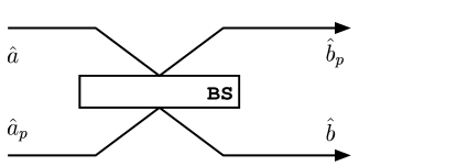
Figure 4.2: Beam splitter

To set $|T|^{2}+|R|^{2}=1$ therefore gives correct annihilation and creation operators and is an energy conservation restriction for a non-absorbing mirror. The expectation values of the number operators after passing the beam splitter are:

$$\langle\hat{n}_{\hat{b}}\rangle = |T|^{2}\langle\hat{n}_{\hat{a}}\rangle+|R|^{2}|\alpha_{p}|^{2}+|TR\alpha_{p}|\cdot\langle\hat{a}e^{i\phi}+\hat{a}^{{\dagger}}e^{-i\phi}\rangle,$$

$$\langle\hat{n}_{\hat{b}_{p}}\rangle = |R|^{2}\langle\hat{n}_{\hat{a}}\rangle+|T|^{2}|\alpha_{p}|^{2}-|TR\alpha_{p}|\cdot\langle\hat{a}e^{i\phi}+\hat{a}^{{\dagger}}e^{-i\phi}\rangle,$$

with $\alpha_{p}$ the coherent state the pump mode $\hat{a}_{p}$ was prepared in, and $\phi$ a combination, $\phi=\phi_{T}-\phi_{R}-\phi_{\alpha_{p}}$, of the phases of the transmission and reflection coefficient and the complex number $\alpha_{p}$ respectively. If we first measure the number of photons coming out in the two modes behind the beam spitter and then subtract them from each other we find the number difference to be:

$$\langle\hat{n}_{\hat{b}}\rangle-\langle\hat{n}_{\hat{b}_{p}}\rangle = 2|TR\alpha_{p}|\langle\hat{a}e^{i\phi}+\hat{a}^{{\dagger}}e^{-i\phi}\rangle$$

$$= \sqrt{2}|TR\alpha_{p}|\langle\hat{x}(\phi)\rangle=\frac{|\alpha_{p}|}{\sqrt{2}}\langle\hat{x}(\phi)\rangle,$$

with, e.g., $|T|=|R|=\frac{1}{\sqrt{2}}$.
For a more accurate calculation involving imperfect photon detectors see Ref. [44], where it is shown that even in this case one can do precise measurements when using a strong local oscillator, e.g., $\alpha_{p}$ is large. The output state and classical information after the homodyne detection is hence a projection of the $N$-mode state on the localised states of the measured mode and the output is a Gaussian $(N-1)$-mode state. To go on we will need the covariance matrix and the displacement vectors of the, about a position $x$, localised state vectors.

4.2.1 Moments of the Localised States

We define the state vectors $|\psi_{x,\epsilon}\rangle$ localised at $x$ with width $\epsilon$.

$$\langle x^{\prime}|\psi_{x,\epsilon}\rangle:=\frac{\exp\left(\frac{-\left(x-x^{\prime}\right)^{2}}{2\epsilon^{2}}\right)}{\sqrt{2\pi\epsilon^{2}}},$$ (4.3)

with

$$tr[|\psi_{x,\epsilon}\rangle\langle\psi_{x,\epsilon}|]=\int_{\mathbbm{R}}\mbox{\rm{d}}x^{\prime}|\langle x^{\prime}|\psi_{x,\epsilon}\rangle|^{2}=\frac{1}{2\epsilon\sqrt{\pi}}.$$

So $|\psi_{x,\epsilon}\rangle$ is not normalised but we find

$$\int_{\mathbbm{R}}\mbox{\rm{d}}x^{\prime}\langle x^{\prime}|\psi_{x,\epsilon}\rangle=1.$$

Let us now calculate the first and second moments of the state vector $|\psi_{x,\epsilon}\rangle$

$$\langle\hat{x}\rangle\,\;\, = \frac{1}{tr[|\psi_{x,\epsilon}\rangle\langle\psi_{x,\epsilon}|]}\int_{\mathbbm{R}}\mbox{\rm{d}}x^{\prime}\langle x^{\prime}|\hat{x}|\psi_{x,\epsilon}\rangle\langle\psi_{x,\epsilon}|x^{\prime}\rangle$$

$$= 2\epsilon\sqrt{\pi}\int_{\mathbbm{R}}\mbox{\rm{d}}x^{\prime}x^{\prime}\frac{\exp\left(\frac{-\left(x-x^{\prime}\right)^{2}}{\epsilon^{2}}\right)}{2\pi\epsilon^{2}}$$

$$= \frac{1}{\epsilon\sqrt{\pi}}\int_{\mathbbm{R}}\mbox{\rm{d}}x^{\prime\prime}\left(x^{\prime\prime}+x\right)\exp\left(\frac{-x^{\prime\prime 2}}{\epsilon^{2}}\right)=x$$

because of the symmetry of the Gaussian.

$$\langle\hat{x}^{2}\rangle\, = 2\epsilon\sqrt{\pi}\int_{\mathbbm{R}}\mbox{\rm{d}}x^{\prime}x^{\prime 2}\frac{\exp\left(\frac{-\left(x-x^{\prime}\right)^{2}}{\epsilon^{2}}\right)}{2\pi\epsilon^{2}}$$

$$= \frac{1}{\epsilon\sqrt{\pi}}\left[2\int_{0}^{\infty}\mbox{\rm{d}}x^{\prime\prime}x^{\prime\prime 2}\exp\left(\frac{-x^{\prime\prime 2}}{\epsilon^{2}}\right)+x^{2}\epsilon\sqrt{\pi}\right]$$

$$= \frac{1}{\epsilon\sqrt{\pi}}\left[\frac{\epsilon^{3}\sqrt{\pi}}{2}+x^{2}\epsilon\sqrt{\pi}\right]=x^{2}+{\epsilon^{2}\over 2},$$

$$\langle\hat{p}\rangle\,\;\, = \frac{1}{tr[|\psi_{x,\epsilon}\rangle\langle\psi_{x,\epsilon}|]}\int_{\mathbbm{R}}\mbox{\rm{d}}x^{\prime}\langle x^{\prime}|\hat{p}|\psi_{x,\epsilon}\rangle\langle\psi_{x,\epsilon}|x^{\prime}\rangle$$

$$= 2\epsilon\sqrt{\pi}\int_{\mathbbm{R}}\mbox{\rm{d}}x^{\prime}\left(-i\frac{\partial\langle x^{\prime}|\psi_{x,\epsilon}\rangle}{\partial x^{\prime}}\right)\langle\psi_{x,\epsilon}|x^{\prime}\rangle$$

$$= -\frac{2i\sqrt{\pi}}{\epsilon}\int_{\mathbbm{R}}\mbox{\rm{d}}x^{\prime}\left(x-x^{\prime}\right)|\langle\psi_{x,\epsilon}|x^{\prime}\rangle|^{2}=0,$$

$$\langle\hat{p}^{2}\,\rangle = 2\epsilon\sqrt{\pi}\int_{\mathbbm{R}}\mbox{\rm{d}}x^{\prime}\left((-i)^{2}\frac{\partial^{2}\langle x^{\prime}|\psi_{x,\epsilon}\rangle}{\partial x^{\prime 2}}\right)\langle\psi_{x,\epsilon}|x^{\prime}\rangle$$

$$= \frac{2\sqrt{\pi}}{\epsilon}\int_{\mathbbm{R}}\mbox{\rm{d}}x^{\prime}\left(1-\frac{\left(x-x^{\prime}\right)^{2}}{\epsilon^{2}}\right)|\langle\psi_{x,\epsilon}|x^{\prime}\rangle|^{2}$$

$$= \frac{1}{2\epsilon^{2}},$$

$$\langle\hat{x}\hat{p}\rangle = \frac{1}{tr[|\psi_{x,\epsilon}\rangle\langle\psi_{x,\epsilon}|]}\int_{\mathbbm{R}}\mbox{\rm{d}}x^{\prime}\,x^{\prime}\left(-i\frac{\partial\langle x^{\prime}|\psi_{x,\epsilon}\rangle}{\partial x^{\prime}}\right)\langle\psi_{x,\epsilon}|x^{\prime}\rangle$$

$$= 2i\epsilon\sqrt{\pi}\int_{\mathbbm{R}}\mbox{\rm{d}}x^{\prime}\frac{\partial\left(x^{\prime}\langle x^{\prime}|\psi_{x,\epsilon}\rangle\right)}{\partial x^{\prime}}\langle\psi_{x,\epsilon}|x^{\prime}\rangle$$

$$= i\epsilon\sqrt{\pi}\int_{\mathbbm{R}}\mbox{\rm{d}}x^{\prime}|\langle x^{\prime}|\psi_{x,\epsilon}\rangle|^{2}=i\epsilon\sqrt{\pi}\frac{1}{2\epsilon\sqrt{\pi}}=\frac{i}{2}$$

$$\langle\hat{p}\hat{x}\rangle = \langle\hat{x}\hat{p}\rangle^{*}=\frac{-i}{2}.$$

The displacement vector and the covariance matrix of the state vector $|\psi_{x,\epsilon}\rangle$ are:

$$\vec{d}_{x,\epsilon} = \left(\begin{array}[]{c}\langle\hat{x}\rangle\\ \langle\hat{p}\rangle\end{array}\right)=\left(\begin{array}[]{c}x\\ 0\end{array}\right),$$

$$\gamma_{x,\epsilon} = \left(\begin{array}[]{cc}2\left(\langle\hat{x}^{2}\rangle-\langle\hat{x}\rangle^{2}\right)&2\langle\hat{x}\hat{p}\rangle-i\\ 2\langle\hat{p}\hat{x}\rangle+i&2\left(\langle\hat{p}^{2}\rangle-\langle\hat{p}\rangle^{2}\right)\end{array}\right)=\left(\begin{array}[]{cc}\epsilon^{2}&0\\ 0&\frac{1}{\epsilon^{2}}\end{array}\right).$$

This result is very convincing since for a well localised state vector $|\psi_{x,\epsilon}\rangle$ with $\epsilon\to 0$, the mean value should be $x$ and the variance of the position should be small. On the other hand we expect the variance of the momentum to grow, following the uncertainty relation. The uncertainty relation can be expressed in terms of the covariance matrix : $\det\gamma\geq 1$ which is in our case fulfilled for every $\epsilon$ : $\det\gamma_{x,\epsilon}=\frac{\epsilon^{2}}{\epsilon^{2}}=1$. To go on we will use the covariance matrix $\Gamma_{x,\epsilon}=\sigma\,\gamma_{x,\epsilon}\,\sigma^{T}=\left(\begin{array}[]{cc}{1\over\epsilon^{2}}&0\\ 0&\epsilon^{2}\end{array}\right)$ and the displacement $\vec{D}_{x,\epsilon}=\sigma\,\vec{d}_{x,\epsilon}=\left(\begin{array}[]{c}0\\ -x\end{array}\right).$

In the real world we can not do precise position measurements since our detectors have imperfect efficiency rates and always some dark counts. If we assume that in the limit of large numbers the measurement outcomes are approximately Gaussian distributed the following argument is true, even when the width $\epsilon$ of the distribution is nonzero.

Schur Complement

We may now calculate what the outcoming state’s covariance matrix is, after realising a projection on an arbitrary Gaussian one-mode state. For $\rho_{AB}$ a Gaussian two-mode state with covariance matrix $\Gamma=\left(\begin{array}[]{cc}A&C\\ C^{T}&B\end{array}\right)$ and displacement $\vec{D}$ we have

$$\chi_{\rho}\left(\xi_{A},\xi_{B}\right):=tr[\hat{W}_{\xi}\,\rho_{AB}]=\exp\left(-\frac{\xi^{T}\Gamma\xi}{4}+i\vec{D}^{T}\xi\right),\,\mbox{ with }\,\xi^{T}=(\xi_{A}^{T}\xi_{B}^{T})\in\mathbbm{R}^{4}.$$

Similarly we have for the Gaussian one-mode state $\omega$ on whom we project a covariance matrix $\Gamma_{\omega}$ and displacement $\vec{D}_{\omega}$

$$\chi_{\omega}\left(\eta_{B}\right):=tr[\hat{W}_{\eta}\omega]=\exp\left(-\frac{\eta^{T}\Gamma_{\omega}\eta}{4}\right),\,\mbox{ with }\,\eta^{T}=\eta_{B}^{T}\in\mathbbm{R}^{4}..$$

With the expansion in Eq. (2.27) the state $\rho^{\prime}$ can be written as:

$$\rho^{\prime} = tr_{B}[\rho_{AB}\,(\hat{\mathbbm{1}}\otimes\omega_{B})]$$

$$= tr_{B}\left[{1\over(2\pi)^{2}}\int\mbox{\rm{d}}^{4}\xi\;\;\chi_{\rho}(-\xi)\hat{W}_{\xi}\;\,\left(\hat{\mathbbm{1}}\otimes{1\over 2\pi}\int\mbox{\rm{d}}^{2}\eta_{B}\;\;\chi_{\omega}(-\eta_{B})\hat{W}_{\eta_{B}}\right)\right]$$

$$= {1\over(2\pi)^{3}}\int\mbox{\rm{d}}^{4}\xi\int\mbox{\rm{d}}^{2}\eta_{B}\;\;\chi_{\rho}(-\xi)\chi_{\omega}(-\eta_{B})\hat{W}_{\xi_{A}}\;tr_{B}[\hat{W}_{\xi_{B}}\hat{W}_{\eta_{B}}],$$

and with the trace formula for the Weyl operators in Lemma 2.3 we have

$$\rho^{\prime} = {1\over 2\pi}\int\mbox{\rm{d}}\xi_{A}\;\left({1\over 2\pi}\int\mbox{\rm{d}}\xi_{B}\;\chi_{\rho}(-\xi)\;\chi_{\omega}(\xi_{B})\right)\;\,\hat{W}_{\xi_{A}}.$$

We find the characteristic function of the output state $\rho^{\prime}$ to be:

$$\chi_{\rho^{\prime}}(-\xi_{A}) = {1\over 2\pi}\int\mbox{\rm{d}}\xi_{B}\;\chi_{\rho}(-\xi)\;\chi_{\omega}(\xi_{B})$$

$$= {1\over 2\pi}\int\mbox{\rm{d}}\xi_{2}\;\exp\left(-\frac{\xi^{T}\Gamma\xi}{4}\right)\exp\left(-\frac{\xi_{B}^{T}\Gamma_{\omega}\xi_{B}}{4}\right)$$

$$\times\exp\left(-i\vec{D}^{T}\xi\right)\;\exp\left(+i\vec{D}^{T}_{\omega}\xi_{B}\right)$$

$$= {1\over 2\pi}\exp\left(-{\xi_{A}^{T}A\xi_{A}\over 4}-i\vec{D}_{A}^{T}\xi_{A}\right)\;\int\mbox{\rm{d}}\xi_{B}\exp\left(-{\xi_{B}^{T}\left(\Gamma_{\omega}+B\right)\xi_{B}\over 4}\right)$$

$$\times\exp\left(-{\xi_{A}^{T}C\xi_{B}\over 2}\right)\exp\left(-i(\vec{D}^{T}_{B}-\vec{D}^{T}_{\omega})\xi_{B}\right).$$

Here we realise that only projections on Gaussian states can transform all Gaussian states again to Gaussian states. If the characteristic function of $\omega$ had third powers of the variable $\xi$ in its exponential, the characteristic function of $\rho^{\prime}$ could take a non-Gaussian form as well, for some Gaussian states $\rho$. We go on and transform the integration variables $\xi_{B}\rightarrow\eta+C^{-1}\xi_{B}$ and include a transformation constant $\mathcal{N}$ and get:

$$\chi_{\rho^{\prime}}(-\xi_{A}) = {\mathcal{N}\over 2\pi}\exp\left(-{\xi_{A}^{T}A\xi_{A}\over 4}-i\vec{D}_{A}^{T}\xi_{A}\right)\exp\left(-{\eta^{T}\left(\Gamma_{\omega}+B\right)\eta\over 4}\right)$$

$$\times\exp\left(-{\xi_{A}^{T}C\eta\over 2}\right)\exp\left(-i(\vec{D}^{T}_{B}-\vec{D}^{T}_{\omega})\eta\right)$$

$$\times\int\mbox{\rm{d}}\xi_{B}\exp\left(-{\xi_{B}^{T}C^{-1T}\left(\Gamma_{\omega}+B\right)C^{-1}\xi_{B}\over 4}\right)$$

$$\times\exp\left(-{\eta^{T}\left(\Gamma_{\omega}+B\right)C^{-1}\xi_{B}\over 2}\right)$$

$$\times\exp\left(-{\xi_{A}^{T}\xi_{B}\over 2}\right)\exp\left(-i(\vec{D}^{T}_{B}-\vec{D}^{T}_{\omega})C^{-1}\xi_{B}\right)$$

and set $\eta=-[\Gamma_{\omega}+B]^{-1}\left(C^{T}\xi_{A}+2i(\vec{D}_{B}-\vec{D}_{\omega})\right)$ so that linear terms of $\xi_{B}$ in the integral vanish and the integral shortens to

$$I=\int\mbox{\rm{d}}\xi_{B}\exp\left(-{\xi_{B}^{T}C^{-1T}\left(\Gamma_{\omega}+B\right)C^{-1}\xi_{B}\over 4}\right)$$

with $I$ being a real number. Using that $B$ and $\Gamma_{\omega}$ are symmetric we finally get:

$$\chi_{\rho^{\prime}}(-\xi_{A}) = {I\mathcal{N}\over 2\pi}\exp\left(-{\xi_{A}^{T}A\xi_{A}\over 4}-i\vec{D}_{A}^{T}\xi_{A}\right)$$

$$\times\exp\left({\xi_{A}^{T}C[\Gamma_{\omega}+B]^{-1}C^{T}\xi_{A}\over 4}\right)\exp\left(i{\xi_{A}^{T}C[\Gamma_{\omega}+B]^{-1}(\vec{D}_{B}-\vec{D}_{\omega})}\right)$$

$$\times\exp\left({-\left(\vec{D}_{B}^{T}-\vec{D}_{\omega}^{T}\right)[\Gamma_{\omega}+B]^{-1}(\vec{D}_{B}-\vec{D}_{\omega})}\right).$$

The $\xi_{A}-$independent factors in $\chi_{\rho^{\prime}}$ have to factor to one since the normalisation condition gives $\chi_{\rho^{\prime}}(0)=1$. Hence

$$\chi_{\rho^{\prime}}(\xi_{A}) = \exp\left(-{\xi_{A}^{T}A\xi_{A}\over 4}+i\vec{D}_{A}^{T}\xi_{A}\right)\exp\left({\xi_{A}^{T}C[\Gamma_{\omega}+B]^{-1}C^{T}\xi_{A}\over 4}\right)$$

$$\times\exp\left(-i{\xi_{A}^{T}C[\Gamma_{\omega}+B]^{-1}(\vec{D}_{B}-\vec{D}_{\omega})}\right).$$

We find the displacement of the state after the projection to be

$$\vec{D}^{\prime}=\vec{D}_{A}-C\left(\Gamma_{\omega}+B\right)^{-1}(\vec{D}_{B}-\vec{D}_{\omega})$$ (4.6)

and the covariance matrix

$$\Gamma^{\prime}=A-C\left(\Gamma_{\omega}+B\right)^{-1}C^{T}.$$ (4.7)

The new $\Gamma^{\prime}$ is a combination of submatrices of $\Gamma$ and is known as the Schur complement of the matrix $B+\Gamma_{\omega}$ in $\tilde{\Gamma}=\Gamma+\left(\begin{array}[]{cc}0&0\\ 0&\Gamma_{\omega}\end{array}\right),$ see Ref. [9]. We will need it in the next chapter when discussing about measuring the degree of entanglement of an unknown state.

Example 8 : Let us calculate $\Gamma^{\prime}$ for the special covariance matrix $\Gamma_{x,\epsilon}=\left(\begin{array}[]{cc}{1\over\epsilon^{2}}&0\\ 0&\epsilon^{2}\end{array}\right)$ of the localised states.

We find with $B=\left(\begin{array}[]{cc}b_{1}&b_{2}\\ b_{2}&b_{3}\end{array}\right)$ the inverse

$$\left(\Gamma_{x,\epsilon}+B\right)^{-1} = \left(\begin{array}[]{cc}b_{1}+{1\over\epsilon^{2}}&b_{2}\\ b_{2}&b_{3}+{\epsilon^{2}}\end{array}\right)^{-1}$$

$$= {\left(\begin{array}[]{cc}b_{3}\epsilon^{2}+\epsilon^{4}&-b_{2}\epsilon^{2}\\ -b_{2}\epsilon^{2}&b_{1}\epsilon^{2}+1\end{array}\right)\over(b_{1}\epsilon^{2}+1)(b_{3}+\epsilon^{2})-\epsilon^{2}b_{2}^{2}}.$$

We finally get the covariance matrix after the projection

$$\Gamma^{\prime}=A-C\,{\left(\begin{array}[]{cc}b_{3}\epsilon^{2}+\epsilon^{4}&-b_{2}\epsilon^{2}\\ -b_{2}\epsilon^{2}&b_{1}\epsilon^{2}+1\end{array}\right)\over(b_{1}\epsilon^{2}+1)(b_{3}+\epsilon^{2})-\epsilon^{2}b_{2}^{2}}\,C^{T}.$$

Since the $\Gamma_{x,\epsilon}$ do not really depend on $x$, $\Gamma^{\prime}$ is the same for every projection on any localised state, while the displacements are different for different projections. For $\epsilon\to 0$ the above inverse becomes the Moore-Penrose inverse, generalising matrix inversion to singular matrices.

4.2.2 Projection on a Coherent State by Homodyne Measurement

In the next chapter we will need an experimentally realisable setup to project one mode of a Gaussian multimode photon state on a coherent state. To do this projection we will use homodyne detection because experimentally it can often be achieved perfectly while other projection strategies are not as efficient.

We discuss the case where the state $\rho$ to be measured has two modes and we want to project it on a coherent state of its second mode. To realise this projection with homodyne measurements we have to find a scheme allowing us to do so. We will show that the following setup is convenient.

Figure 4.3: Measurement setup

The mathematical description of this processing is done by unitaries followed by homodyne measurements in the second and third mode.

$$\langle\psi_{y,\epsilon}|_{C}\,\langle\psi_{x,\epsilon}|_{B}\,\hat{U}^{P}_{C}\,\hat{U}^{BS}_{BC}\;(\rho_{AB}\,\otimes|0\rangle\langle 0|_{C})\;\hat{U}^{{\dagger}\,BS}_{BC}\,\hat{U}^{{\dagger}\,P}_{C}\,|\psi_{x,\epsilon}\rangle_{B}\,|\psi_{y,\epsilon}\rangle_{C}.$$

With all of these ingredients being Gaussian we can identify the outcoming state by using only the covariance matrix representation of all operations. We start with a two mode state $\rho$ having an arbitrary covariance matrix $\Gamma=\left(\begin{array}[]{cc}A&C\\ C^{T}&B\end{array}\right)$ and displacement $\vec{D}=\left(\begin{array}[]{c}\vec{D}_{A}\\ \vec{D}_{B}\end{array}\right)$, the vacuum $|0\rangle\langle 0|$ with CM $\Gamma_{0}=\mathbbm{1}$ and vanishing displacement (see Section 3.1). We will also need the localised states, with width $\epsilon$, realised by the homodyne measurements all having the covariance matrix $\Gamma_{\epsilon}=\left(\begin{array}[]{cc}{1\over\epsilon^{2}}&0\\ 0&\epsilon^{2}\end{array}\right)$ and different displacements $\vec{D}_{x}=\left(\begin{array}[]{c}0\\ -x\end{array}\right).$ We apply a $50:50$ beam splitter described by the symplectic transformation

$$S^{BS}={1\over\sqrt{2}}\left(\begin{array}[]{cc}\mathbbm{1}&-\mathbbm{1}\\ \mathbbm{1}&\mathbbm{1}\end{array}\right),$$

a one mode ${\pi\over 2}-$phase shifter

$$S^{P}_{\pi\over 2}=\left(\begin{array}[]{cc}0&1\\ -1&0\end{array}\right)=\sigma$$

and send two modes to homodyne measurement boxes. We calculate step by step what happens on the covariance matrix and the displacement of $\rho$ passing this setup.

operation	displacement and covariance matrix
adding the vacuum as a third mode	$\displaystyle\vec{D}\mapsto\vec{D}^{\prime}=\left(\begin{array}[]{c}\vec{D}_{A}\\ \vec{D}_{B}\\ 0\end{array}\right)$ $\displaystyle\Gamma\mapsto\Gamma^{\prime}=\left(\begin{array}[]{ccc}A&C&0\\ C^{T}&B&0\\ 0&0&\mathbbm{1}\end{array}\right)$
beam splitter operation on the second and third mode	$\displaystyle\vec{D}^{\prime}\mapsto$ $\displaystyle\vec{D}^{\prime\prime}$ $\displaystyle=S^{BS}\vec{D}^{\prime}=\left(\begin{array}[]{c}\vec{D}_{A}\\ {1\over\sqrt{2}}\vec{D}_{B}\\ {1\over\sqrt{2}}\vec{D}_{B}\end{array}\right)$ $\displaystyle\Gamma^{\prime}\mapsto$ $\displaystyle\Gamma^{\prime\prime}$ $\displaystyle=S^{BS}\,\Gamma^{\prime}\,S^{T\,BS}=\left(\begin{array}[]{ccc}A&{C\over\sqrt{2}}&{C\over\sqrt{2}}\\ {C^{T}\over\sqrt{2}}&{B+\mathbbm{1}\over 2}&{B-\mathbbm{1}\over 2}\\ {C^{T}\over\sqrt{2}}&{B-\mathbbm{1}\over 2}&{B+\mathbbm{1}\over 2}\end{array}\right)$
phase shifter operation on the third mode	$\displaystyle\vec{D}^{\prime\prime}$ $\displaystyle\mapsto$ $\displaystyle\vec{D}^{\prime\prime\prime}=S^{P}_{\pi\over 2}\,\vec{D}^{\prime\prime}=\left(\begin{array}[]{c}\vec{D}_{A}\\ \!\!\!\!{1\over\sqrt{2}}\vec{D}_{B}\\ {1\over\sqrt{2}}\sigma\vec{D}_{B}\end{array}\right)$ $\displaystyle\Gamma^{\prime\prime}$ $\displaystyle\mapsto$ $\displaystyle\Gamma^{\prime\prime\prime}=S^{P}_{\pi\over 2}\,\Gamma^{\prime\prime}\,S^{P\,T}_{\pi\over 2}=\left(\begin{array}[]{ccc}A&{C\over\sqrt{2}}&{C\sigma^{T}\over\sqrt{2}}\\ {C^{T}\over\sqrt{2}}&\;\;{B+\mathbbm{1}\over 2}&\;\;{B-\mathbbm{1}\over 2}\sigma^{T}\\ {\sigma C^{T}\over\sqrt{2}}&\sigma{B-\mathbbm{1}\over 2}&\sigma{B+\mathbbm{1}\over 2}\sigma^{T}\end{array}\right)$
homodyne measurement on the second mode with the outcome $x$	$\displaystyle\vec{D}^{\prime\prime\prime}$ $\displaystyle\mapsto$ $\displaystyle\vec{D}^{(4)}=\left(\begin{array}[]{c}\vec{D}_{A}\\ {1\over\sqrt{2}}\sigma\vec{D}_{B}\end{array}\right)$ $\displaystyle\quad-\left(\begin{array}[]{c}{C\over\sqrt{2}}\\ \sigma{B-\mathbbm{1}\over 2}\end{array}\right)\left[{B+\mathbbm{1}\over 2}+\Gamma_{\epsilon}\right]^{-1}\left[{1\over\sqrt{2}}\vec{D}_{B}-\vec{D}_{x}\right]$ $\displaystyle\Gamma^{\prime\prime\prime}$ $\displaystyle\mapsto$ $\displaystyle\Gamma^{(4)}=\left(\begin{array}[]{cc}A&{C\sigma^{T}\over\sqrt{2}}\\ {\sigma C^{T}\over\sqrt{2}}&\sigma{B+\mathbbm{1}\over 2}\sigma^{T}\end{array}\right)$ $\displaystyle\quad-\left(\begin{array}[]{c}{C\over\sqrt{2}}\\ \sigma{B-\mathbbm{1}\over 2}\end{array}\right)\left[{B+\mathbbm{1}\over 2}+\Gamma_{\epsilon}\right]^{-1}\left(\begin{array}[]{cc}{C^{T}\over\sqrt{2}}&{B-\mathbbm{1}\over 2}\sigma^{T}\end{array}\right)$

We abbreviate

$$M = M^{T}={\left[{B+\mathbbm{1}\over 2}+\Gamma_{\epsilon}\right]^{-1}\over 2}$$

$$= {\left(\begin{array}[]{cc}1+b_{3}+2\epsilon^{2}&-b_{2}\\ -b_{2}&1+b_{1}+{2\over\epsilon^{2}}\end{array}\right)\over\det B+b_{3}(1+{2\over\epsilon^{2}})+b_{1}(1+2\epsilon^{2})+2(\epsilon+{1\over\epsilon})^{2}+1}.$$

And get for $\vec{D}^{(4)}$:

$$\vec{D}^{(4)}=\left(\begin{array}[]{c}\vec{D}_{A}-{\sqrt{2}CM}\left[{1\over\sqrt{2}}\vec{D}_{B}-\vec{D}_{x}\right]\\ {1\over\sqrt{2}}\sigma\vec{D}_{B}-\sigma(B-\mathbbm{1})M\left[{1\over\sqrt{2}}\vec{D}_{B}-\vec{D}_{x}\right]\end{array}\right)$$

and for $\Gamma^{(4)}$ we find:

$$\Gamma^{(4)} = \left(\begin{array}[]{cc}A-{CM}{C^{T}}&{C\over\sqrt{2}}\left(\mathbbm{1}-{M}(B-\mathbbm{1})\right)\sigma^{T}\\ \sigma\left(\mathbbm{1}-(B-\mathbbm{1})M\right){C^{T}\over\sqrt{2}}&{\sigma\left[(B+\mathbbm{1})-(B-\mathbbm{1})M(B-\mathbbm{1})\right]\sigma^{T}\over 2}\end{array}\right).$$

As the last step we implement a homodyne measurement on the former third mode with the outcome $y$. The final displacement and covariance matrix are given by

$$\vec{D}^{(4)} \mapsto \vec{D}^{(5)}=\vec{D}_{A}-{CM\sqrt{2}}\left[{1\over\sqrt{2}}\vec{D}_{B}-\vec{D}_{x}\right]-{C\over\sqrt{2}}\left(\mathbbm{1}-M(B-\mathbbm{1})\right)\sigma^{T}$$

$$\qquad\qquad\quad\times\left[{\sigma\left[(B+\mathbbm{1})-(B-\mathbbm{1})M(B-\mathbbm{1})\right]\sigma^{T}\over 2}+\Gamma_{\epsilon}\right]^{-1}$$

$$\qquad\qquad\qquad\quad\times({1\over\sqrt{2}}\sigma\vec{D}_{B}-\sigma(B-\mathbbm{1})M\left[{1\over\sqrt{2}}\vec{D}_{B}-\vec{D}_{x}\right]-\vec{D}_{y}),$$

$$\Gamma^{(4)} \mapsto \Gamma^{(5)}=A-CMC^{T}-{C\over\sqrt{2}}\left(\mathbbm{1}-M(B-\mathbbm{1})\right)\sigma^{T}$$

$$\qquad\qquad\qquad\qquad\times\left[{\sigma\left[(B+\mathbbm{1})-(B-\mathbbm{1})M(B-\mathbbm{1})\right]\sigma^{T}\over 2}+\Gamma_{\epsilon}\right]^{-1}$$

$$\qquad\qquad\qquad\qquad\qquad\times\sigma\left(\mathbbm{1}-(B-\mathbbm{1})M\right){C^{T}\over\sqrt{2}}$$

Surprisingly this expression reduces to

$$\Gamma^{(5)} = A-C\left[B+\mathbbm{1}\right]^{-1}C^{T},$$ (4.22)

where no $\epsilon$ appear anymore, meaning that even a huge width of a Gaussian distributed measurement outcome is not relevant for the resulting covariance matrix. From the covariance matrix and the displacement of the resulting state $\rho^{\prime}$ we can read off that it would have been the same to project the initial state $\rho$ on coherent state vectors $|\alpha(x,y,\epsilon)\rangle$. The complex number $\alpha$ depends on the outcomes of the homodyne measurements: $x$ and $y$, and on the Gaussian detection distribution with width $\epsilon$, with all those quantities appearing in $\vec{D}^{(5)}$.

Chapter 5 Measuring Entanglement of Two-Mode States

To determine whether a given unknown Gaussian two-mode state is entangled or not and how much, one can measure all entries of the covariance matrix, i.e., ten real numbers. But since we only want to know a special property of the state it could be that fewer measurements are necessary to answer the same question. We propose a scheme which makes it possible to determine the symplectic eigenvalues of the partially transposed covariance matrix with nine measurements. In the two-mode case, where the PPT criterion is necessary and sufficient, these symplectic eigenvalues are adequate to find out the degree of entanglement, measured in the logarithmic negativity.

5.1 Measurement Scheme

Given an unknown covariance matrix $\gamma$ of a Gaussian two-mode state $\gamma=\left(\begin{array}[]{cc}A&C\\ C^{T}&B\end{array}\right)$ with $A,B$ real symmetric and $C$ real $2\times 2$ matrices.

Step 1

Measure all entries of $A=\left(\begin{array}[]{cc}a_{1}&a_{2}\\ a_{2}&a_{3}\end{array}\right)$ and determine $a=\sqrt{\det A}=a_{1}a_{3}-a_{2}^{2}$. Experimentally this can be done by simple position and momentum measurements with homodyne detection. The measurement outcomes of a position/momentum measurement will approximately be Gaussian distributed. The variance of the measured distribution is an estimator for the covariance matrix element $a_{1}$/$a_{3}$. To measure the off-diagonal element $a_{2}$ we apply a ${\pi\over 4}-$phase shifter $S^{P}_{\pi\over 4}={1\over\sqrt{2}}\left(\begin{array}[]{cc}1&-1\\ 1&1\end{array}\right)$ so that the diagonal element $A_{11}$ transforms to a linear combination of all elements of $A$ namely $A^{\prime}_{11}=a_{1}+a_{3}-2a_{2}$. When measuring the position of the transformed state one will approximately get a Gaussian distribution with variance $A^{\prime}_{11}$ from which we can determine the value of $a_{2}$.

Step 2

Measure all entries of $B=\left(\begin{array}[]{cc}b_{1}&b_{2}\\ b_{2}&b_{3}\end{array}\right)$ and determine $b=\sqrt{\det B}=b_{1}b_{3}-b_{2}^{2}.$

Step 3

Calculate and implement the local symplectic transformation which brings $A$ and $B$ to their diagonal form.

$$S=S_{A}\oplus S_{B}:\gamma\mapsto\gamma^{\prime}=S\gamma S^{T}=\left(\begin{array}[]{cc}a\mathbbm{1}&C^{\prime}\\ C^{\prime T}&b\mathbbm{1}\end{array}\right)$$

with $C^{\prime}=S_{A}CS^{T}_{B}$. The experimental setup depends on the matrices $A$ and $B$ but the transformations $S_{A}$ and $S_{B}$ are generally phase shifters with variable phase $\phi$ :   $P_{\phi}=\left(\begin{array}[]{cc}\cos\phi&-\sin\phi\\ \sin\phi&\cos\phi\end{array}\right)$ which should be available for every $\phi$.

Step 4

As we saw in Subsection 4.2.2 it is possible to project a two (or more) mode system on coherent states of its second mode using homodyne measurements. Although the projections done with the proposed setup change with the measurement outcomes of the homodyne boxes, it is always a projection on a coherent state. The CM of the measured state changes in every case according to

$$\gamma^{\prime}\mapsto\gamma^{\prime\prime}=a\mathbbm{1}-(b+1)^{-1}C^{\prime}C^{\prime T}.$$

giving a proper one-mode covariance matrix. Apply the projection physically.

Remark: The different displacements of the coherent states have no effect on the covariance matrix but only on the displacement the resulting state has.

Step 5

Measure all entries of $\gamma^{\prime\prime}=\left(\begin{array}[]{cc}g_{1}&g_{2}\\ g_{2}&g_{3}\end{array}\right)$. Since $\gamma^{\prime\prime}$ is symmetric we only have to measure three times, one less as when measuring the non-symmetric matrix $C$. Calculate the matrix $C^{\prime}C^{\prime T}=(b+1)(-\gamma^{\prime\prime}+a\mathbbm{1})$ and the absolute value of $\det C$:

$$\det(C^{\prime}C^{\prime T}) = (\det C^{\prime})^{2}=(\det S_{A}CS^{T}_{B})^{2}$$

$$= (\det C)^{2}=(b+1)^{2}[(a-g_{1})(a-g_{3})-g_{2}^{2}].$$

Step 6

With the following calculation we determine the determinant of the initial $\gamma$:

$$\det \left[\left(\begin{array}[]{cc}\mathbbm{1}&-{1\over b}C^{\prime}\\ 0&\mathbbm{1}\end{array}\right)\left(\begin{array}[]{cc}a\mathbbm{1}&C^{\prime}\\ C^{\prime T}&b\mathbbm{1}\end{array}\right)\left(\begin{array}[]{cc}\mathbbm{1}&0\\ -{1\over b}C^{\prime T}&\mathbbm{1}\end{array}\right)\right]$$

$$= \det\left[\left(\begin{array}[]{cc}a\mathbbm{1}-{1\over b}C^{\prime}C^{\prime T}&0\\ 0&b\mathbbm{1}\end{array}\right)\right]=b^{2}\det\left[a\mathbbm{1}-{1\over b}C^{\prime}C^{\prime T}\right]$$

$$= \det\left[(b+1)\gamma^{\prime\prime}-a\mathbbm{1}\right]\overset{!}{=}\det\gamma^{\prime}=\det\gamma.$$

Step 7

We now know the Simon normal form of the matrix $\gamma$ namely

$$\gamma^{SNF}=\left(\begin{array}[]{cccc}a&0&c&0\\ 0&a&0&d\\ c&0&b&0\\ 0&d&0&b\end{array}\right)$$

with $a$ from Step 1, $b$ (2) and $c,d$ determined by the equations $cd=\det C$ (5) and $\det\gamma=a^{2}b^{2}+c^{2}d^{2}-ab(c^{2}+d^{2})$ (6). There is a little ambiguity in 5 since the sign of the determinant of $C$ is not fixed.

5.2 Determining the Degree of Entanglement

We remember that every two-mode covariance matrix can be brought to Simon normal form only by local symplectic transformations which do not change the degree of entanglement. The symplectic eigenvalues of the covariance matrix in Simon normal form are

$$(\gamma^{SNF})_{1,2}={1\over\sqrt{2}}\sqrt{a^{2}+b^{2}+2cd\pm\sqrt{(a^{2}+b^{2}+2cd)^{2}-4\det\gamma}}.$$ (5.3)

To decide whether the given state $\gamma$ is entangled or not we use the PPT-criterion stating that an entangled Gaussian state must have a partial transpose which violates the uncertainty relation for covariance matrices. The symplectic eigenvalues of the partially transposed CM can be calculated using again the Simon invariants via :

$$(\gamma^{SNF})^{T_{A}}_{1,2}={1\over\sqrt{2}}\sqrt{a^{2}+b^{2}-2cd\pm\sqrt{(a^{2}+b^{2}-2cd)^{2}-4\det\gamma}}.$$ (5.4)

From the preceding steps we have all ingredients to determine the values of $(\gamma^{SNF})_{1,2}$ and $(\gamma^{SNF})^{T_{A}}_{1,2}$ with the little subtlety that we do not know the sign of $cd$. We first take the positive sign for $\det C$ and calculate all eigenvalues. If all eigenvalues in Eq. (5.3) and (5.4) are greater than one, the state was not entangled. This does not change when taking the negative sign of $\det C$ since the eigenvalues of $(\gamma^{SNF})^{T_{A}}$ and $\gamma^{SNF}$ then just interchange. We hence know that the state is not entangled but can not decide if the state has Simon normal form

$$\gamma^{SNF_{1}}=\left(\begin{array}[]{cccc}a&0&c&0\\ 0&a&0&d\\ c&0&b&0\\ 0&d&0&b\end{array}\right)\mbox{ or }\gamma^{SNF_{2}}=\left(\begin{array}[]{cccc}a&0&-c&0\\ 0&a&0&d\\ -c&0&b&0\\ 0&d&0&b\end{array}\right).$$

If one of the eigenvalues was smaller than one then this eigenvalue belongs to $(\gamma^{SNF})^{T_{A}}$ and the state is entangled. In fact we are able to determine the degree of entanglement the state posses with only nine measurements instead of ten when measuring the whole state. The exact degree of entanglement can be calculated with Eq. (3.25)

$$E_{\mathcal{N}}(\gamma)=-\sum_{i}\min(\ln\gamma_{i}^{T_{A}},0).$$

and the symplectic eigenvalues from above.

5.3 Discussion of the Measurement Strategies

To experimentally realise a measurement is often a really expensive adventure, but the costs could be reduced when performing less measurements. The easiest way to determine the symplectic eigenvalues of a covariance matrix would be to measure just all elements of the CM; that makes ten different kinds of measurements. But why not learn from the available results of previous measurements? As we showed in the previous steps, it is possible to get the symplectic eigenvalues with less queries, when adjusting the strategy dependent on the information we already gained. For future work, a challenging task would be the optimisation of such strategies. One could even try to proof how many kinds of measurements one necessarily has to perform to determine the symplectic eigenvalues of the covariance matrix of a given state, when it is allowed to learn during the process.

But maybe our strategy is not that good because the variances of the measured covariance matrix entries could be worse as in the ten number case. It could be, that when measuring all entries of the CM one has to measure every entry $N_{10}$ times to get the same results and the same variances as with our nine number idea for $N_{9}>>N_{10}$ measurements. The energy saved when only measuring nine instead of ten entries is then spend on more tries for every element.

We simulated both strategies, assuming that $\gamma$ is the matrix

$$\gamma=\left(\begin{array}[]{cccc}3.5&0&2.5&0\\ 0&3&0&-2.5\\ 2.5&0&3.5&0\\ 0&-2.5&0&3\end{array}\right).$$

The calculated symplectic eigenvalues of the given $\gamma$ are

$$\gamma_{1}=2.345\quad\gamma_{2}=1.732$$ (5.5)

and the symplectic eigenvalues of $\gamma^{T_{A}}$ are given by

$$\gamma^{T_{A}}_{1}=0.707\quad\gamma^{T_{A}}_{2}=5.745,$$ (5.6)

thus $\gamma$ is entangled. To determine the entries of the covariance matrix we simulated $N=10^{2},10^{3},10^{4},10^{5},10^{6}$ measurements in total. For the usual ten number strategy we measured every entry $N_{10}={N\over 10}$ times, while for the nine number strategy we measured every single quantity $N_{9}={N\over 9}$ times. The estimations of the entries of the covariance matrix where done using ten (nine) Gaussian probability distributions, centered about zero. The variances of the first four Gaussians where the diagonal entries of the covariance matrix $\gamma$, which one can experimentally determine by position or momentum measurements. For the off-diagonal entries one first has to apply phase shifters, to bring them on the diagonal. Measuring again the position of such a transformed state gave values for those entries. For every expectation value we took the average over all $N$ measurements and calculated the variance of the measurement outcomes. These results are the estimators for the covariance matrix entries. The whole procedure was done $M$ times for $M=1000$ measurements. From the estimated covariance matrix we calculated the symplectic eigenvalues of $\gamma$ and $\gamma^{T_{A}}$, each $M$ times, using Eq. (5.3) and Eq. (5.4) respectively and got an estimator for each of them. We compared the average of these measurement outcomes to the exact values and found the following result.

With the usual ten measurements the estimation of the smallest symplectic eigenvalue $\gamma_{1}^{T_{A}}$, from which one can determine the degree of entanglement of the Gaussian state, was a bit better. The decrease of the abberation of the estimated symplectic eigenvalue in comparison to the exact value was approximatly equal in both strategies. The standard deviation of the measured $\gamma^{T_{A}}_{1}$ from the exact one, is calculated using the $M$ estimated values of $\gamma^{T_{A}}_{1}$

$$\Delta\gamma_{1}^{T_{A}}=\sqrt{{1\over M-1}\,\sum_{i=1}^{M}\,\left[(\gamma^{T_{A}}_{1})_{i}-(\gamma^{T_{A}}_{1})_{exact}\right]^{2}}$$ (5.7)

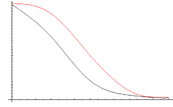
$\Delta\gamma_{1}^{T_{A}}$

0.6                            nine kinds

0.5                                    of measurements

0.4

0.3          ten kinds

0.2         of measurements

0.1

0

2                 3                 4                5                 6       $\log_{10}N$

Figure 5.1: Ten Measurements versus Nine

The figure shows the standard deviation $\Delta\gamma_{1}^{T_{A}}$ for the ten measurement strategy (lower curve) and the nine measurement strategy (upper curve). The behaviour of the variances for the total number of measurements $N=10^{2},10^{3},10^{4},10^{5},10^{6}$ is shown on a logarithmic scale. Unfortunately our nine measurement strategy gives worse results than the ten measurement strategy. With increasing $N$ the variances of the symplectic eigenvalue $\gamma_{1}^{T_{A}}$ estimated with the two strategies decreases, as it should be.

5.4 Collective Measurements

Finally we note, that it is by no means clear that single mode measurements, as we employed in the proposed setup, turn out to give better measurement strategies than a measurement using more copies of a state. Sometimes it can be useful to implement collective measurements, meaning that not only one copy of a state is measured but two or more copies are merged and processed together. The measurements of those multimode states could allow to further reduce the number of queries. We often want to know only a special quantity composed of entries of the covariance matrix. In this case, with collective measurements it is indeed possible to reduce the number of measurements, as the following example shows.

Example 9 : Let $\gamma$ be a two-mode covariance matrix of the form

$$\gamma=\left(\begin{array}[]{cc}A&C\\ C^{T}&B\end{array}\right).$$

We are interested in the determinant of $A+B$ and would naively measure the three entries of each matrix $A$ and $B$. Employing collective measurements instead could give the desired determinant with only three measurements, as the following strategy shows. Take two copies of a state with covariance matrix $\gamma$ and apply a beam splitter

$\left(\begin{array}[]{cccc}\mathbbm{1}&0&0&0\\ 0&{\mathbbm{1}\over\sqrt{2}}&-{\mathbbm{1}\over\sqrt{2}}&0\\ 0&{\mathbbm{1}\over\sqrt{2}}&{\mathbbm{1}\over\sqrt{2}}&0\\ 0&0&0&\mathbbm{1}\end{array}\right)\left(\begin{array}[]{cccc}A&C&0&0\\ C^{T}&B&0&0\\ 0&0&A&C\\ 0&0&C^{T}&B\end{array}\right)\left(\begin{array}[]{cccc}\mathbbm{1}&0&0&0\\ 0&{\mathbbm{1}\over\sqrt{2}}&{\mathbbm{1}\over\sqrt{2}}&0\\ 0&-{\mathbbm{1}\over\sqrt{2}}&{\mathbbm{1}\over\sqrt{2}}&0\\ 0&0&0&\mathbbm{1}\end{array}\right)$

$={1\over 2}\left(\begin{array}[]{cccc}2~{}A&\sqrt{2}~{}C&\sqrt{2}~{}C&0\\ \sqrt{2}~{}C^{T}&B+A&B-A&-\sqrt{2}~{}C\\ \sqrt{2}~{}C&B-A&B+A&\sqrt{2}~{}C\\ 0&-\sqrt{2}~{}C^{T}&\sqrt{2}~{}C^{T}&2~{}B\end{array}\right).$

We can just measure the three entries of the principal matrix $B+A$, where for the offdiagonal entry of $B+A$ one has to implement an additional ${\pi\over 4}-$phase shifter on the second mode. With these three measurements we can calculate the determinant without knowing what the independent values of $A$ and $B$ are. We hence saved half of the costs with just a little trick.

Chapter 6 Entanglement Witnesses

We explain how separability can be formulated on covariance matrix level and introduce the advantageous concept of entanglement witnesses (EW). We propose a scheme to efficiently estimate the degree of entanglement of an unknown state by realisable experimental measurements. Global reference is the script on Gaussian states, Ref. [45], to be published.

6.1 Separability

We review some basic properties of covariance matrices and formulate another separability criterion on the CMs. First, we recall the definition of separability of states and extend it to $M$ parties.

Definition 6.1 (Separability)

A state $\rho$ is separable with respect to $M$ parties iff it can be written (or approximated, e.g., in trace norm), with probabilities $p_{i}\geq 0$ and $\sum_{i}p_{i}=1$ and proper density matrices $\rho_{i}^{(j)}$ belonging to the $j$th party, as

$$\rho=\sum_{i}p_{i}\,\rho_{i}^{(1)}\otimes\ldots\otimes\rho_{i}^{(M)},$$

that is, the closed convex hull of the $M$-product states.

Fortunately the separability of states can be formulated on the level of their covariance matrices with the following theorem, proved in Ref. [48].

Theorem 6.1 (Separability of CMs)

Let $\gamma$ be the covariance matrix of a state $\rho$, which is separable with respect to $M$ parties. Then there exist proper covariance matrices $\gamma^{(1)},\ldots,\gamma^{(M)}$ corresponding to the $M$ parties, such that

$$\gamma\geq\gamma^{(1)}\oplus\ldots\oplus\gamma^{(M)}.$$

Conversely, if this condition is satisfied, then the Gaussian state with covariance matrix $\gamma$ is separable. If the stated relation is fulfilled by a CM we will name the covariance matrix itself separable with respect to the $M$ parties.

Proof : For the first statement let the state $\rho$ be decomposed $\rho=\sum_{i}p_{i}\,\rho^{i}$ where all $\rho^{i}$ are $M$-product states and with probabilities $p_{i}\geq 0,\,\sum_{i}p_{i}=1$. For $\gamma$ covariance matrix and $\vec{d}$ displacement vector of the state $\rho$ it is

$$tr[\rho\,\{\hat{R}_{k}-\langle\hat{R}_{k}\rangle,\hat{R}_{l}-\langle\hat{R}_{l}\rangle\}_{+}]=\gamma_{kl}+2d_{k}d_{l}=\sum_{i}p_{i}(\gamma_{kl}^{i}+2d_{k}^{i}d_{l}^{i}),$$

where the $\gamma^{i}$ are the block diagonal covariance matrices (Lemma 3.2) $\gamma^{i}=\bigoplus_{j=1}^{M}(\gamma^{i})^{(j)}$ and $\vec{d}^{i}$ the first moments of the $\rho^{i}$.

The difference $\Delta_{kl}=\gamma_{kl}-\sum_{i}p_{i}\gamma_{kl}^{i}=2\sum_{i}p_{i}\,d_{k}^{i}d_{l}^{i}-2d_{k}d_{l}$ is a positive definite matrix, since for every $\vec{v}\in\mathbbm{R}^{2N}$ it is

$$(\vec{v},\Delta\vec{v}) = 2\sum_{i}p_{i}\,\sum_{kl}v_{k}d_{k}^{i}d_{l}^{i}v_{l}-2\sum_{kl}v_{k}d_{k}d_{l}v_{l}$$

$$= 2\sum_{i}p_{i}\,|(\vec{v},\vec{d}^{i})|^{2}-2|(\vec{v},\vec{d})|^{2}$$

and with $\vec{d}=\sum_{i}p_{i}\vec{d}^{i}$ we get

$$(\vec{v},\Delta\vec{v}) = 2\sum_{i}p_{i}\,|(\vec{v},\vec{d}^{i})|^{2}-2\left|\sum_{i}p_{i}(\vec{v},\vec{d}^{i})\right|^{2}$$

$$\geq 2\sum_{i}p_{i}\,|(\vec{v},\vec{d}^{i})|^{2}-2\sum_{i}p_{i}^{2}|(\vec{v},\vec{d}^{i})|^{2}$$

$$= 2\sum_{i}p_{i}\,|(\vec{v},\vec{d}^{i})|^{2}(1-p_{i})\geq 0.$$

Thus it is indeed possible to find a direct sum of proper covariance matrices $\gamma^{(1)}\oplus\ldots\oplus\gamma^{(M)}$, namely the $\gamma^{(j)}:=\left(\sum_{i}p_{i}\gamma^{i}\right)^{(j)}$, that fulfil the stated relation since

$$\gamma = \sum_{i}p_{i}\gamma^{i}+\Delta\geq\sum_{i}p_{i}\left[\bigoplus_{j=1}^{M}(\gamma^{i})^{(j)}\right]=\bigoplus_{j=1}^{M}\left[\left(\sum_{i}p_{i}\gamma^{i}\right)^{(j)}\right].$$

In order to proof the second part of the theorem let $\gamma$ be a covariance matrix

$$\gamma=\bigoplus_{j=1}^{M}\gamma^{(j)}+\Delta,$$

with an arbitrary positive matrix $\Delta$ and $\lambda$ a (classical) normalised, about zero centred Gaussian probability distribution in $\mathbbm{R}^{2N}$ with covariance matrix ${\Delta\over 2}$ :

$$\lambda(\eta)=\mathcal{N}\,e^{-{\eta^{T}{1\over\Delta}\eta}},$$

let $\omega$ be a density operator describing a Gaussian state with block diagonal covariance matrix $\bigoplus_{j=1}^{M}\gamma^{(j)}$ and vanishing displacement. The expansion of $\omega$ then reads

$$\omega={1\over(2\pi)^{N}}\int\mbox{\rm{d}}^{2N}\xi\;e^{-{\xi^{T}\sigma\left[\bigoplus_{j=1}^{M}\gamma^{(j)}\right]\sigma^{T}\xi\over 4}}\;\hat{W}_{\xi}$$

where we have used the relation $\Gamma=\sigma\gamma\sigma^{T}$. We construct the state $\rho$ with $\lambda$ and $\omega$ :

$$\rho:=\int\mbox{\rm{d}}^{2N}\!\!\eta\,\,\lambda(\eta)\,\hat{W}^{{\dagger}}_{\eta}\,\omega\,\hat{W}_{\eta},$$

and find that it is a Gaussian state with covariance matrix $\gamma$ since its characteristic function is of the form :

$$\chi_{\rho}(\xi) = tr[\rho\,\hat{W}_{\xi}]=\int\mbox{\rm{d}}^{2N}\!\!\eta\,\,\lambda(\eta)\,tr[\hat{W}^{{\dagger}}_{\eta}\,\omega\,\hat{W}_{\eta}\hat{W}_{\xi}]$$

$$= tr[\omega\,\hat{W}_{\xi}]\int\mbox{\rm{d}}^{2N}\!\!\eta\,\,\lambda(\eta)\,e^{-i\eta^{T}\sigma\xi}$$

$$= e^{-{\xi^{T}\sigma[\bigoplus_{j=1}^{M}\gamma^{(j)}]\sigma^{T}\xi\over 4}}\,e^{-{\xi^{T}\sigma\Delta\sigma^{T}\xi\over 4}}=e^{-{\xi^{T}\sigma\gamma\sigma^{T}\xi\over 4}}.$$

We now have to proof that $\rho$ is separable with respect to the $M$ parties. We will need the following lemma to complete the proof:

Lemma 6.1

Let $C$ be a closed convex set, $\rho$ be a $C$ valued function and $g$ be a continuous strictly positive function $g:\mathbbm{R}\to\mathbbm{R}^{+}$ with $\int_{-\infty}^{+\infty}\mbox{\rm{d}}t\,g(t)=1$. Then the integral

$$\int_{-\infty}^{+\infty}\mbox{\rm{d}}t\,g(t)\,\rho(t)$$ (6.1)

is again an element of $C$.

Proof : Let $G$ be the integral of $g$, that is $G^{\prime}=g$, which is strictly monotonically increasing and $G:\mathbbm{R}\to[0,1]$. We observe that the integral Eq. (6.1) can be substituted to the form

$$\int_{-\infty}^{+\infty}\mbox{\rm{d}}t\,g(t)\,\rho(t)=\int_{-\infty}^{+\infty}\mbox{\rm{d}}t\,G^{\prime}(t)\,\rho(t)=\int_{0}^{1}\mbox{\rm{d}}x\,\rho(G^{-1}(x)).$$

By definition of the Riemann integral that is equal to

$$\lim_{\begin{subarray}{c}N\to\infty\\ \Delta x_{i}\to 0\end{subarray}}\quad\sum_{i=1}^{N}\rho(G^{-1}(x_{i}))\Delta x_{i},$$ (6.2)

with $0=x_{1}\leq x_{2}\leq\ldots x_{N+1}=1$ and $\Delta x_{i}=x_{i+1}-x_{i}\geq 0$ and hence $\sum_{i=1}^{N}\Delta x_{i}=1$. The sum in Eq. (6.2) is a convex combination and thus an element of C. Since C is closed the limit is reached in $C$. $\Box$

In our problem the multi-dimensional function $\lambda$ can be brought to product form by orthogonal diagonalization. Its factors are then indeed continuous, normalised and strictly positive functions. Furthermore all $\omega_{\eta}:=\hat{W}^{{\dagger}}_{\eta}\,\omega\,\hat{W}_{\eta}$ are product states, because the covariance matrix of $\omega$ is of block diagonal form, and hence separable, while the operators $\hat{W}_{\eta}$ only displace $\omega$ without affecting its covariance matrix. We use the previous lemma iteratively and find that the state $\rho=\int\mbox{\rm{d}}^{2N}\!\!\eta\,\,\lambda(\eta)\,\omega_{\eta}$ is separable. This completes the proof of the theorem. $\Box$

Definition 6.2

We define the closed convex sets
$\Gamma(\mathbbm{R}^{2N})$ = Set of covariance matrices $\gamma$, elements of $Sym(2N,\mathbbm{R})$ with the properties $\gamma\geq 0$ and $\gamma\pm i\sigma\geq 0$. $\Gamma_{A|B}(\mathbbm{R}^{2N})$ = Set of separable covariance matrices $\gamma\in\Gamma(\mathbbm{R}^{2N})$ ( with respect to the split $A|B$), with $\gamma\geq\gamma_{A}\oplus\gamma_{B}$ for some $\gamma_{A}\in\Gamma(\mathbbm{R}^{2N_{A}}),\gamma_{B}\in\Gamma(\mathbbm{R}^{2N_{B}})$ with $N=N_{A}+N_{B}$ .

Definition 6.3

The principal submatrices $A_{r}$ of a square matrix $A$ are the matrices which result when one neglects one or more columns and rows always of the same number.

Lemma 6.2

Let $\gamma$ be a covariance matrix, element of $\Gamma(\mathbbm{R}^{2N})$ $\left(\Gamma_{A|B}(\mathbbm{R}^{2N})\right)$ , $P$ a positive matrix and $\alpha\geq 1$ then

$$1. \gamma^{\prime}=\gamma+P$$

$$2. \gamma^{\prime\prime}=\alpha\gamma$$

are still elements of $\Gamma(\mathbbm{R}^{2N})$ $\left(\Gamma_{A|B}(\mathbbm{R}^{2N})\right)$ and

$$3. \mbox{ all principal submatrices of }\gamma\mbox{ containing }N_{r}\mbox{ modes}$$

are elements of $\Gamma(\mathbbm{R}^{2N_{r}})$ $\left(\Gamma_{A|B}(\mathbbm{R}^{2N_{r}})\right)$.

Proof : $1.$ Is obvious.
$2.\,\gamma^{\prime\prime}$ is still a real positive matrix. The uncertainty relation is fulfilled for $\alpha\geq 1$ since $\alpha\gamma+i\sigma=(\alpha-1)\gamma+(\gamma+i\sigma)\geq 0$. If $\gamma$ was separable with $\gamma\geq\gamma_{A}\oplus\gamma_{B}$, $\gamma^{\prime\prime}$ is still separable since $\gamma^{\prime\prime}\geq\alpha\gamma_{A}\oplus\alpha\gamma_{B}$ with proper covariance matrices $\alpha\gamma_{A}$ and $\alpha\gamma_{B}$.
$3.$ All principal submatrices of a positive matrix $A$ are always positive since for all $v\in\mathbbm{R}^{2N}:\langle v|A|v\rangle\geq 0$. Especially for all $v_{r}$ in the reduced spaces $\mathbbm{R}^{2N_{r}}$ with $N_{r}\leq N$. Then $0\leq\langle v_{r}|A|v_{r}\rangle=\langle v_{r}|A_{r}|v_{r}\rangle$ where the $A_{r}$ are the principal submatrices of $A$ depending on the reduction one chose. That applies for $\gamma_{r}$ and also for $\gamma_{r}+i\sigma_{r}$, so that $\gamma_{r}$ is again a CM on $\Gamma(\mathbbm{R}^{2N_{r}})$. Additionally the positive matrix $\gamma-\gamma_{A}\oplus\gamma_{B}$ stays positive for reductions on $N_{r}$ modes. $\Box$

6.2 Entanglement Witnesses

A relatively new method to distinguish separable from entangled states results from the insight that the set of covariance matrices and the set of separable CMs form closed convex subsets of the space of real symmetric $2N\times 2N$ matrices. The convexity allows to describe these subsets completely by the intersection of closed half-spaces or equivalently by a family of linear inequalities. One family of such inequalities is given by the so called entanglement witnesses. They were first proposed in Ref. [46], further investigations can be found in Ref. [47] on discrete states and on continuous states in Ref. [45]. We consider bipartite CVS systems and start with the definition of appropriate entanglement witnesses.

Definition 6.4

We define the following sets of real symmetric $2N\times 2N$-matrices

$$\mathcal{Z}(\mathbbm{R}^{2N}) = \{Z|\,\forall\gamma\in\Gamma(\mathbbm{R}^{2N}):\,tr[\gamma\,Z]\geq 1\}$$

$$\mathcal{Z}_{A|B}(\mathbbm{R}^{2N}) = \{Z|\forall\gamma\in\Gamma_{A|B}(\mathbbm{R}^{2N}):\,tr[\gamma\,Z]\geq 1,\}$$

where $A|B$ denotes the split of a bipartite system with $N=N_{A}+N_{B}$ modes and $\gamma$ covariance matrix. All matrices $Z\in\mathcal{Z}_{A|B}(\mathbbm{R}^{2N})$ will be called entanglement witnesses for the split $A|B$.

The defined sets are again closed convex subsets with $\mathcal{Z}(\mathbbm{R}^{2N})\subset\mathcal{Z}_{A|B}(\mathbbm{R}^{2N})$. Furthermore it is possible to assign to every entanglement witness a quadratic Hamiltonian.

Definition 6.5

Let $Z$ be an element of $\mathcal{Z}_{A|B}(\mathbbm{R}^{2N})$ and $\hat{R}=(\hat{x}_{1},\ldots,\hat{p}_{N}).^{T}$ We define the Hamiltonian

$$\hat{Z}[\hat{R}]:=2\sum_{k,l=1}^{N}Z_{kl}\hat{R}_{k}\hat{R}_{l}.$$

With the help of the trace we see how the matrix $Z$ is related to the expectation value of the operator $\hat{Z}$. Let $\gamma$ be the covariance matrix and $\vec{d}$ the displacement of a state $\rho$. The expectation value of any $\hat{Z}$ can be expressed in terms of the moments of the state:

$$\langle\hat{Z}[\hat{R}]\rangle_{\rho} = tr[\hat{Z}[\hat{R}]\,\rho]=2\sum_{k,l=1}^{N}Z_{kl}\,tr[\hat{R}_{k}\hat{R}_{l}\,\rho]$$ (6.3)

$$= \sum_{k,l=1}^{N}Z_{kl}(\gamma_{kl}+2d_{k}d_{l})=tr[Z\gamma]+2\vec{d}^{T}Z\vec{d}.$$

In the following lemma we see how entanglement witnesses detect entangled states.

Lemma 6.3

For $\gamma$ covariance matrix of a bipartite system of $N_{A}+N_{B}=N$ modes, it is:

$$\gamma\,\mbox{ is separable } \iff \forall Z\in\mathcal{Z}_{A|B}(\mathbbm{R}^{2N})\,:tr[Z\gamma]\geq 1$$

with respect to the split $A|B$.

For Gaussian states only the covariance matrix determines the entanglement properties, thus a separable covariance matrix is necessary and sufficient for a Gaussian state $\rho$ to be separable. For non-Gaussian states it is necessary to have a separable covariance matrix but not sufficient since higher moments could show entanglement. The lemma for non-Gaussian states is thus

$$\exists Z\in\mathcal{Z}_{A|B}(\mathbbm{R}^{2N}):\,tr[Z\gamma]<1 \iff \gamma\,\mbox{ is entangled }$$

$$\Rightarrow$$ all CV states having the covariance

$$\mbox{ matrix }\gamma\mbox{ are entangled.}$$

Proof : $\Rightarrow$ is clear from the definition of entanglement witnesses in Def. 6.4. In order to prove the $\Leftarrow$ direction we will need an important theorem from the theory of convex sets which can be found in [49] given here without proof:

Theorem 6.2 (Separation of point from convex set)

Let $Y$ be a closed, convex, nonempty set of matrices, $Y\subset Sym(2N,\mathbbm{R})$, let $x\in Sym(2N,\mathbbm{R})\backslash Y$. Then there exists a matrix $M\in Sym(2N,\mathbbm{R}),\,M\not=0$ with

$$tr[Mx]<\min_{y\in Y}\,tr[My].$$

The set of separable covariance matrices $\Gamma_{A|B}(\mathbbm{R}^{2N})$ is such a closed convex set. In order to prove Lemma 6.3 we assume to have an entangled $x$ and show that there has to exist a $Z\in\mathcal{Z}_{A|B}(\mathbbm{R}^{2N})$ which then detects it and gives $tr[Z\,x]<1$.

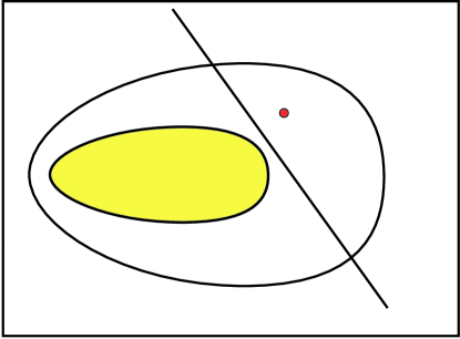
$x$

$\Gamma_{A|B}(\mathbbm{R}^{2N})$

$\Gamma(\mathbbm{R}^{2N})$

$Sym(2N,\mathbbm{R})$                      $M$

Figure 6.1: Separation of point from convex set

With Theorem 6.2 we find a matrix $M\in Sym(2N,\mathbbm{R})$ so that

$$tr[M\,x]<c=\min_{\gamma^{\prime}\in\Gamma_{A|B}(\mathbbm{R}^{2N})}\,tr[M\,\gamma^{\prime}]\leq tr[M\,\gamma]\quad\forall\,\gamma\in\Gamma_{A|B}(\mathbbm{R}^{2N}).$$ (6.4)

Let us assume that the real number $c$ is strictly positive. Then we get $tr[{M\over c}\,x]<1\leq tr[{M\over c}\,\gamma]\quad\forall\,\gamma\,\Gamma_{A|B}(\mathbbm{R}^{2N})$ but if this is true ${M\over c}=Z$ has to be an element of $\mathcal{Z}_{A|B}(\mathbbm{R}^{2N})$, since it is a real symmetric matrix with the defining condition in Def. 6.4. We have found that if we take an $x\not\in\Gamma_{A|B}(\mathbbm{R}^{2N})$ we will find an $Z\in\mathcal{Z}_{A|B}(\mathbbm{R}^{2N})$ which gives $tr[Z\,x]<1$ or equivalently $\forall Z\in\mathcal{Z}_{A|B}(\mathbbm{R}^{2N}):tr[Z\,\gamma]\geq 1\Rightarrow\gamma\in\Gamma_{A|B}(\mathbbm{R}^{2N})$.

We still have to discuss the case $c\leq 0$. Let us show that $M$ is positive by contradiction. Suppose $M$ were not positive and had an eigenvalue $m_{0}<0$ with the corresponding eigenvector $\mu\in\mathbbm{R}^{2N}$. We construct the matrix $\gamma^{\prime}_{kl}=\gamma_{kl}+\lambda\mu_{k}\mu_{l}$ for an arbitrary $\lambda\geq 0$ and a separable matrix $\gamma$, which by Lemma 6.2 is itself an element of $\Gamma_{A|B}(\mathbbm{R}^{2N})$. We find that $tr[M\gamma^{\prime}]=tr[M\gamma]+\lambda\,m_{0}\,\mu^{2}\to-\infty$ for $\lambda\to\infty$. With this construction we see that $M$ cannot have any eigenvalue smaller than zero because Eq. (6.4) has to hold and $tr[M\,\gamma^{\prime}]=tr[M\,\gamma]+\lambda m_{0}\mu^{2}$ would reach values smaller than $tr[Mx]$ for sufficiently large $\lambda$. Hence $M$ is positive.
But then the following equation holds for every $\gamma\in\Gamma_{A|B}(\mathbbm{R}^{2N})$:

$$tr[M\gamma] = tr[M\,S\,\gamma^{WNF}\,S^{T}]=tr[S^{T}\,M\,S\,\gamma^{WNF}]$$

$$= tr[S^{T}\,M\,S\,(\gamma^{WNF}-\mathbbm{1})]+tr[S^{T}\,M\,S]$$

$$> 0,$$

since the first addend is again the trace of a (semi-)positive matrix, see Eq. (3.19) and Lemma 2.1, while the second addend is the trace of a positive matrix which is only zero if all eigenvalues of it were zero that is the matrix $S^{T}\,M\,S$ and hence the matrix $M$ itself was the zero matrix. But Theorem 6.2 excluded the $M=0$ case. We conclude that there exists at least one nonzero $M\in Sym(2N,\mathbbm{R})$ so that for all $\gamma\in\Gamma_{A|B}(\mathbbm{R}^{2N})$ we find a strictly positive $c$. This completes the proof of Lemma 6.3. $\Box$

Definition 6.6

The symplectic trace (denoted as $str[A]$ ) of an even dimensional, positive, symmetric matrix $A$ is defined as the sum of the symplectic eigenvalues (counted once).

Lemma 6.4

Let $A=\left(\begin{array}[]{cc}A_{1}&A_{2}\\ A_{2}^{T}&A_{3}\end{array}\right)$ denote a real positive $2N\times 2N$ matrix, then the symplectic trace has the following properties:

$$str[S\,A\,S^{T}] = str[A]\quad\forall S\in Sp(2N,\mathbbm{R})\quad\mbox{invariance }$$

$$str[pA] = p\,str[A]\quad p\geq 0\quad\mbox{multiplicity}$$

$$str[A] \leq str[A_{1}]+str[A_{3}]$$

Proof : The invariance is clear since symplectic transformations preserve all symplectic eigenvalues, additionally the symplectic eigenvalues just all multiply with the factor $p$ so that multiplicity holds. The last property can be derived as a consequence of Theorem 6.3. $\Box$

But given a real symmetric $2N\times 2N$ matrix, is it an entanglement witness or not? The following theorem answers the question providing a check, based on the symplectic eigenvalues the given matrix possesses.

Theorem 6.3

Let $Z$ be a real symmetric $2N\times 2N$ matrix on a phase space of $N=N_{A}+N_{B}$ modes. Let $Z_{A}$ and $Z_{B}$ denote the principal submatrices of $Z$ belonging to the subsystems $A$ and $B$ respectively. Then :
$\begin{array}[]{lcl}\qquad\qquad 1.\,Z\in\mathcal{Z}(\mathbbm{R}^{2N})&\iff&Z\geq 0\;\mbox{and }\>str[Z]\geq{1\over 2}\\ \qquad\qquad 2.\,Z\in\mathcal{Z}_{A|B}(\mathbbm{R}^{2N})&\iff&Z\geq 0\;\mbox{and }\>str[Z_{A}]+str[Z_{B}]\geq{1\over 2}.\end{array}$

Note that $str[Z]\geq{1\over 2}$ is stronger than $str[Z_{A}]+str[B]\geq{1\over 2}$.

Proof : (following reference [45])
$1.\Rightarrow$ : With the same argument as in the proof of Lemma 6.3 we find that $Z\in\mathcal{Z}(\mathbbm{R}^{2N})$ has to be positive. Since $Z\geq 0$ we can find a symplectic transformation to bring $Z$ to Williamson normal form:

$$Z^{WNF}=S_{z}\,Z\,S_{z}^{T}=Z_{0}\oplus\bigoplus_{i}\left(\begin{array}[]{cc}z_{i}&0\\ 0&z_{i}\end{array}\right)$$

where $Z_{0}$ is a matrix with determinant zero and zero symplectic eigenvalues. We assume that the particular $Z$ has a vanishing $Z_{0}$ part an go on. The symplectic trace of $Z$ is now easily calculated: $str[Z]=str[Z^{WNF}]=\sum_{i}z_{i}$. Furthermore we have with the basis transformation $\hat{R}^{\prime}\mapsto\hat{R}=S_{z}\hat{R}^{\prime}$

$$\ tr[\hat{Z}[\hat{R}^{\prime}]\rho^{\prime}] = tr[\hat{Z}^{WNF}[\hat{R}]\rho]=2\sum_{i}\left(\langle Q_{i}^{2}\rangle_{\rho}+\langle P_{i}^{2}\rangle_{\rho}\right)z_{i}$$ (6.5)

$$= 2\sum_{i}\left(2\langle\hat{n}_{i}\rangle_{\rho}+1\right)z_{i}\,\geq 2\,str[Z],$$

where $\hat{n}_{i}=\hat{a}_{i}^{{\dagger}}\hat{a}_{i}$. The right hand side is the expectation value of the Hamiltonian of harmonic oscillators which is bounded from below by the ground state energy reached when $\rho$ in Eq. (6.5) was the ground state.

On the other hand the expectation value of $\hat{Z}$ is related to the state’s moments via $tr[\hat{Z}[\hat{R}^{\prime}]\rho^{\prime}]=tr[Z\gamma^{\prime}]+2\,\vec{d}^{\prime T}\,Z\,\vec{d}^{\prime}\geq tr[Z\gamma^{\prime}]\geq 1$ for all $\gamma^{\prime}\in\Gamma(\mathbbm{R}^{2N}),\,\rho^{\prime}\in S(\mathcal{H})$ by Def. 6.4. Since the boundary in Eq. (6.5) is reached, we conclude the stated property of $Z$, namely $2\,str[Z]\geq 1$. Also for all $Z^{\prime}$ identical to $Z$ but with a nonzero $Z_{0}$ part it follows $str[Z^{\prime}]=str[Z]\geq{1\over 2}$.

$1.\Leftarrow$ : For all $\gamma\in\Gamma(\mathbbm{R}^{2N})$ and with $Z^{WNF}$ again Williamson normal form of $Z$, including a $Z_{0}$ part, we calculate:

$$tr[Z\,\gamma] = tr[S^{T}\,Z^{WNF}S\gamma]=tr[Z_{0}\gamma^{\prime}_{0}]+\sum_{i}tr[z_{i}\mathbbm{1}\gamma^{\prime}_{i}]$$

$$\geq \sum_{i}z_{i}(\lambda_{i}^{1}+\lambda_{i}^{2}),$$

where $\gamma^{\prime}_{0}$ and $\gamma^{\prime}_{i}$ are the principal submatrices of $\gamma^{\prime}$. $\gamma^{\prime}_{0}$ has the size of $Z_{0}$ while all $\gamma^{\prime}_{i}$ are $2\times 2$ covariance matrices with the positive eigenvalues $\lambda_{i}^{1}$ and $\lambda_{i}^{2}$ which fulfil $\lambda_{i}^{1}\cdot\lambda_{i}^{2}\geq 1$ for every submatrix since the determinant of $\gamma^{\prime}_{i}$ is necessarily greater or equal to one. And since for every $\lambda\geq 0$ the relation $0\leq(\sqrt{\lambda}-{1\over\sqrt{\lambda}})^{2}=\lambda+{1\over\lambda}-2$ holds, it follows that

$$\forall\gamma\in\Gamma(\mathbbm{R}^{2N}):\,tr[Z\,\gamma]\geq\sum_{i}z_{i}(\lambda_{i}^{1}+{1\over\lambda_{i}^{1}})\geq 2\sum_{i}z_{i}=2\,str[Z]\geq 1.$$

Thus $Z$ is an element of $\mathcal{Z}(\mathbbm{R}^{2N})$ as stated.

$2.\Rightarrow$ : For $Z\in\mathcal{Z}_{A|B}(\mathbbm{R}^{2N})$ we run the above argument (proof of Lemma 6.3) for the positivity. For a separable $\gamma$ we have the useful condition proved in Theorem 6.1: $\gamma\geq\gamma_{A}\oplus\gamma_{B}$ for some covariance matrices $\gamma_{A}$ and $\gamma_{B}$. Thus

$$tr[Z\gamma]\geq tr[Z_{A}\gamma_{A}]+tr[Z_{B}\gamma_{B}]\geq 0$$

and with Eq. (6.3) and $\rho_{A},\rho_{B}$ the Gaussian states with covariance matrix $\gamma_{A},\gamma_{B}$ respectively and vanishing displacement, follows

$$tr[Z\gamma] = tr[\hat{Z}_{A}[\hat{R}]\rho_{A}]+tr[\hat{Z}_{B}[\hat{R}]\rho_{B}].$$

Additionally it is $Z_{A},Z_{B}\geq 0$ and hence $tr[\hat{Z}_{A}[\hat{R}]\rho_{A}]\geq 2\,str[Z_{A}]$ and $tr[\hat{Z}_{B}[\hat{R}]\rho_{B}]\geq 2\,str[Z_{B}]$ from above, so we get

$$tr[Z\gamma] \geq 2\,str[Z_{A}]+2\,str[Z_{B}]$$

reached again when both subsystems are in ground state. By the precondition we also have $tr[Z\gamma]\geq 1$ for all $\gamma\in\Gamma_{A|B}(\mathbbm{R}^{2N})$ so that the condition on the symplectic trace of the entanglement witness is

$$2str[Z_{A}]+2str[Z_{B}]\geq 1.$$

$2.\Leftarrow$ : We use the same idea as for $1.\Leftarrow$. For all $\gamma\in\Gamma_{A|B}(\mathbbm{R}^{2N})$ and $Z^{WNF}_{A}$ and $Z^{WNF}_{B}$ the symplectic diagonalized submatrices of $Z$ it is :

$$tr[Z\,\gamma] \geq tr[Z_{A}\gamma_{A}]+tr[Z_{B}\gamma_{B}]=tr[Z^{WNF}_{A}\gamma^{\prime}_{A}]+tr[Z^{WNF}_{B}\gamma^{\prime}_{B}]$$

$$= tr[Z^{A}_{0}\gamma^{\prime A}_{0}]+\sum_{i\in A}tr[z^{A}_{i}\,\mathbbm{1}\,\gamma^{\prime A}_{i}]$$

$$\qquad\qquad\qquad+tr[Z^{B}_{0}\gamma^{\prime B}_{0}]+\sum_{i\in B}tr[z^{B}_{i}\,\mathbbm{1}\,\gamma^{\prime B}_{i}]$$

$$\geq 2\,\sum_{i\in A}z^{A}_{i}+2\,\sum_{i\in B}z^{B}_{i}=2\,str[Z_{A}]+2\,str[Z_{B}]\,\geq\,1,$$

finally completing the proof. $\Box$

We have now a powerful tool to decide whether a given matrix is an entanglement witness for the given split $A|B$ or not. And with them we can restrict the sets a given covariance matrix is an element of. The picture shows how two entanglement witnesses $Z_{1}$ and $Z_{2}$ divide the set of covariance matrices in $\mathbbm{R}^{2N}$ into four subsets.

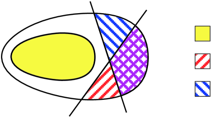
separable covariance matrices

trace of $Z_{1}\gamma$ is smaller than $1$

trace of $Z_{2}\gamma$ is smaller than $1$

$\Gamma(\mathbbm{R}^{2N})$

$Z_{1}\qquad\quad Z_{2}$

Figure 6.2: Entanglement witnesses dividing $\Gamma(\mathbbm{R}^{2N})$

If the trace of the given CM $\gamma$ together with the entanglement witness $Z_{1}$ ($Z_{2}$) was smaller than one, then $\gamma$ belongs to the red-lined (blue-lined) set respectively. If both measurements gave values smaller than one, it is in the squared set. In those cases all states having the covariance matrix $\gamma$ are entangled. If, on the other hand, both entanglement witnesses gave values greater than one, we can not say whether the given matrix is entangled or not. But from the geometric representation we guess that optimal entanglement witnesses going exactly through the edge between separable with entangled CMs, exist and indeed they do. We will not introduce them here but only give references [50].

6.3 Estimation of the Degree of Entanglement

We now come to the main results of this thesis. We have so far learned a lot about Gaussian states, their covariance matrices and their entanglement properties. When producing a Gaussian two-mode state in the lab usually one wants to make sure that the outcoming state behind the particular setup is really the desired state. Especially it is often necessary to check whether the state has the expected entanglement properties used for quantum cryptography or other purposes. For that reason one is interested in a simple measurement scheme telling the experimenter immediately what degree of entanglement the produced state has. In the third chapter we learned that for Gaussian states entanglement, quantified in the logarithmic negativity, can easily be calculated using only the covariance matrices of the states. So it should be possible to measure some properties of a CM and give an estimate of the degree of entanglement for the Gaussian states having this particular covariance matrix. In the previous section we introduced the concept of entanglement witnesses and saw that they are very practical and provide a natural way to distinguish separable from entangled states. But one could do even better. It is not only possible to decide whether a state is entangled or not but with practicable measurements one can estimate a lower bound of entanglement of a given unknown Gaussian state. We show how this can be done and start off with the definition of $p-$separability.

Definition 6.7

For any $\gamma\in\Gamma(\mathbbm{R}^{2N})$ covariance matrix of a bipartite system $A|B$ and any $p\in(0,1]$ we define

$$\gamma\mbox{ is }p-\mbox{separable}\iff{\gamma\over p}\mbox{ is separable}$$

with respect to the split $A|B$ respectively. The sets of $p-$separable covariance matrices are again closed, convex subsets of $\Gamma(\mathbbm{R}^{2N})$ and will be denoted by $\Gamma^{p}_{A|B}(\mathbbm{R}^{2N})$.

The definition is sensible since $\,{\gamma\over p}$ with Lemma 6.2 and $\alpha={1\over p}\geq 1$  still has covariance matrix properties. Note, that by definition separability is equal to $1-$separability and for $p_{1}\geq p_{2}$ follows: $\gamma\mbox{ is }p_{1}-\mbox{separable}\Rightarrow\gamma\mbox{ is }p_{2}-\mbox{separable}$ and the sets $\Gamma^{p}_{A|B}(\mathbbm{R}^{2N})$ include each other like the shells of an onion $\Gamma^{1}_{A|B}(\mathbbm{R}^{2N})\subset\Gamma^{0.5}_{A|B}(\mathbbm{R}^{2N})\subset\Gamma^{0.2}_{A|B}(\mathbbm{R}^{2N})\subset\Gamma(\mathbbm{R}^{2N}),$ as shown in the figure.

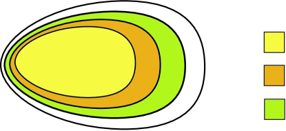
$(1-)$ separable CM

$0.5-$separable CM

$0.2-$separable CM

$\Gamma(\mathbbm{R}^{2N})$

Figure 6.3: $p-$Separability

Using the definition of $p-$separability Theorem 6.1 can be reformulated to

Theorem 6.4 ($p-$Separability of CMs)

Let $\gamma$ be a, with respect to the two parties $A$ and $B$, $p-$separable covariance matrix, i.e. $\gamma\in\Gamma^{p}_{A|B}(\mathbbm{R}^{2N})$. Then there exist proper covariance matrices $\gamma^{A}\in\Gamma(\mathbbm{R}^{2N_{A}})$ and $\gamma^{B}\in\Gamma(\mathbbm{R}^{2N_{B}})$ corresponding to the parties, such that

$$\gamma\geq p\,\,(\gamma^{A}\oplus\gamma^{A}).$$

And finally, $p-$separability of covariance matrices can easily be expressed with entanglement witnesses as the following lemma shows:

Lemma 6.5

For $\gamma$ CM of a bipartite system, $p\in(0,1]$ and $Z$ being an entanglement witnesses, we find the relation:

$$\gamma\mbox{ is }p-\mbox{separable }(A|B) \iff \,\forall Z\in\mathcal{Z}_{A|B}(\mathbbm{R}^{2N}):\,tr[Z\gamma]\geq p$$

$$\negthinspace\negthinspace\negthinspace\negthinspace\negthinspace\negthinspace\negthinspace\negthinspace\negthinspace\negthinspace\negthinspace\negthinspace\negthinspace\negthinspace\negthinspace\negthinspace\negthinspace\negthinspace\negthinspace\negthinspace\negthinspace\negthinspace\negthinspace\negthinspace\mbox{ or }\quad\gamma\mbox{ is not }p-\mbox{separable }(A|B) \iff \,\exists Z\in\mathcal{Z}_{A|B}(\mathbbm{R}^{2N}):\,tr[Z\gamma]<p.$$

Proof : With the definition of $p-$separability, Theorem 6.1 and Lemma 6.3 the stated relations follow immediately. $\Box$

For $p<1$, $p-$separability is weaker than the usual separability, but when blown up with a factor ${1\over p}$ they would reach the set of separable covariance matrices $\Gamma_{A|B}(\mathbbm{R}^{2N})$. In this sense, the smaller the number $p$ is, the more entangled can the covariance matrix be. We observe, that when measuring an entanglement witness $Z$, the outcome $p=tr[Z\gamma]$ does not only distinguish separable ($p\geq 1$ for all witnesses) from entangled ($p<1$ for one particular witness) covariance matrices, furthermore it orders the entangled CMs in sets of $p-$separable CMs.

An experimenter who produces Gaussian states with a certain degree of entanglement is naturally curious if he succeeded in doing so. When he measures an entanglement witness $Z_{0}$ on a given unknown Gaussian state $\rho$ having a vanishing displacement and covariance matrix $\gamma$ the outcome is given by

$$m=\langle\hat{Z}_{0}[\hat{R}\,]\rangle_{\rho}=tr[Z_{0}\gamma]<p:=m+\epsilon,\quad\forall\,\epsilon>0.$$

The measurement outcome tells him now immediately that the state is not $p-$separable for all $\epsilon>0$. But maybe this is not the best estimate he could do. It is possible that with a different entanglement witness a smaller outcome $m$ could be measured and the state would be even more entangled. Since he produced the Gaussian state $\rho$, it is not completely unknown to him; he actually has a strong conjecture what the state will be and can use his knowledge to find an minimal entanglement witness for the covariance matrix associated to the state $\rho$. In contrast to optimal entanglement witnesses it is not the witness going exactly through the edge between entangled and separable states, but it is the one that gives the best estimate of the degree of entanglement the supposed state has. Obviously the minimal entanglement witnesses depend on the covariance matrix for whom they are minimal. We will understand the minimal entanglement witnesses $Z_{min}(\gamma)$ to a given bipartite CM $\gamma$ as being those witnesses $Z_{min}(\gamma)\in\mathcal{Z}_{A|B}(\mathbbm{R}^{2N}),$ which give

$$tr[Z_{min}(\gamma)\,\gamma]=p_{min}(\gamma),$$

while all other EWs $Z\in\mathcal{Z}_{A|B}(\mathbbm{R}^{2N})$ give $tr[Z\gamma]>\,p_{min}$. The number $p_{min}(\gamma)$ is then the smallest value of the outcomes $p$, one could measure for the CM $\gamma$.

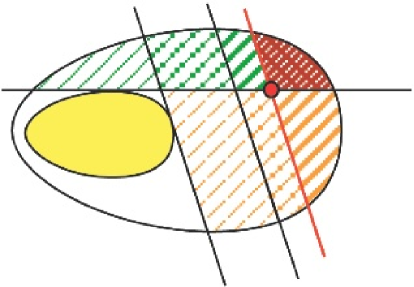
$Z_{opt}$

$\gamma_{0}$

$Z_{min}(\gamma_{0})$

$\Gamma(\mathbbm{R}^{2N})$

$Z_{opt}$     $Z$

Figure 6.4: Optimal and minimal entanglement witnesses

In Fig. 6.4 the coloured areas are those where entanglement witnesses gave values smaller than one, so the CMs in these areas must be entangled. The minimal EW $Z_{min}(\gamma_{0})$ gave $tr[Z_{min}(\gamma_{0})\,\gamma_{0}]=p_{min}(\gamma_{0})$ for the covariance matrix $\gamma_{0}$, symbolised by the red dot.

We see that it should be possible to give lower bounds for the degree of entanglement of a Gaussian state using entanglement witnesses. To estimate the degree of entanglement quantified in the logarithmic negativity, we will need that the PPT-criterion is necessary and sufficient, which is the case in $1_{A}\times N_{B}$ mode systems. We learned in Lemma 3.6 that the logarithmic negativity of a Gaussian state can be calculated from its covariance matrix:

$$E_{\mathcal{N}}(\gamma)=-\sum_{i}\min(\ln\gamma_{i}^{T_{A}},0).$$ (6.6)

In the following lemma all the things we learned are merged together and we find how the outcomes of the measurements of entanglement witnesses bind the logarithmic negativity of the measured state.

Lemma 6.6

In case the PPT-criterion is necessary and sufficient:
If an experimental setup measuring the trace of an entanglement witness $Z$ with a covariance matrix $\gamma$ belonging to an unknown Gaussian $N-$ mode state gave the outcome $m\in(0,1)$, the logarithmic negativity of the state is bounded from below by

$$E_{\mathcal{N}}(\gamma) \geq \ln{1\over m}.$$

In the two-mode case, where only one symplectic eigenvalue of $\gamma^{T_{A}}$ can be smaller than one, the minimal witness $Z_{min}$ giving the smallest possible value $m_{min}$ gives exactly the logarithmic negativity the state possesses.

Proof : With the symplectic eigenvalues of the partially transposed covariance matrix $\gamma^{T_{A}}$ defined in Eq. (3.3) and Lemma 6.5 we see that forall $p\in(0,1]$

$$\forall i:\gamma_{i}^{T_{A}}\geq 1\! \iff \!\gamma\mbox{ is separable }\quad\mbox{(PPT!),}$$

$$\forall i:\gamma_{i}^{T_{A}}\geq p\! \iff \!\gamma\mbox{ is }p-\mbox{separable }\!\iff\forall Z\in\mathcal{Z}_{A|B}(\mathbbm{R}^{2N}):tr[Z\gamma]\geq p,$$

$$\exists i:\gamma_{i}^{T_{A}}<p\! \iff \!\gamma\mbox{ is not }p-\mbox{separable}\!\iff\exists Z\in\mathcal{Z}_{A|B}(\mathbbm{R}^{2N}):tr[Z\gamma]<p.$$

From the measurement we know that there exists an entanglement witness giving the result $m$. We hence know that there exists at least one symplectic eigenvalue $\gamma^{T_{A}}_{1}$ of $\gamma^{T_{A}}$ which is smaller than $p=m+\epsilon$ for all $\epsilon>0$. Thus we can give a nontrivial lower bound for the logarithmic negativity of the state.

$$E_{\mathcal{N}}(\gamma) = -\sum_{i=2}^{N}\min(\ln\gamma_{i}^{T_{A}},0)-\min(\ln\gamma_{1}^{T_{A}},0)$$

$$> -\ln p=\ln{1\over m+\epsilon}$$

and since this inequality is true for $p=m+\epsilon,\;\forall\epsilon>0$, the proof of the first statement is complete. For the second part we assume a symplectic eigenvalue $\gamma_{1}^{T_{A}}$ smaller than one and we get

$$E_{\mathcal{N}}(\gamma) = -\min(\ln\gamma_{2}^{T_{A}},0)-\min(\ln\gamma_{1}^{T_{A}},0)$$

$$= 0+\ln{1\over\gamma_{1}^{T_{A}}}.$$

Since the outcome of our measurement gave the value $m_{min}$ for the given covariance matrix, we conclude that the symplectic eigenvalue $\gamma_{1}^{T_{A}}$ is smaller than or equal to $m_{min}$. On the other hand by definition of the minimal measurement outcome $m_{min}$ it is for all $Z\in Z_{A|B}(\mathbbm{R}^{2N}):\,tr[Z\gamma]\geq m_{min}$ and hence for all symplectic eigenvalues $\gamma_{i}^{T_{A}}\geq m_{min}$. Hence $\gamma_{1}^{T_{A}}$ is equal to $m_{min}$ and the logarithmic negativity is given as stated. $\Box$

The lemma provides an easy method to estimate a lower bound of entanglement by measuring different entanglement witnesses. The estimated logarithmic negativity becomes larger the smaller the minimal measurement outcome was, respecting the ordering induced by the sets of $p-$separable covariance matrices. Entanglement witnesses also detect bound entangled states, being those entangled states having a positive partial transpose. If existent, they destroy the sufficiency of the PPT-criterion and measured in terms of the logarithmic negativity they have a vanishing degree of entanglement. Unless bound entangled states exist the logarithmic negativity is strictly positive for entangled covariance matrices. A possible goal for future research could be a computable entanglement measure also respecting the $p-$ordering but giving nonzero values for bound entangled states.

Summarising our achievements, we see that an experimenter, wanting to know the degree of entanglement his produced Gaussian state possesses, simply has to measure some entanglement witnesses and the results instantly tell him how much the state is minimally entangled. With little additional knowledge about the state it is furthermore possible to optimise the measurements, trying only minimal entanglement witnesses. In the following example we see that sometimes even the knowledge of the structure of the covariance matrix is sufficient to determine minimal entanglement witnesses for it.

Example 10 : Let $\gamma$ be of the special form

$$\gamma=\left(\begin{array}[]{cccc}a&0&b&0\\ 0&a&0&-b\\ b&0&a&0\\ 0&-b&0&a\end{array}\right)\quad\mbox{ with }a\geq 1\mbox{ and }0\leq b\leq a.$$

Then the symplectic eigenvalues of the $\gamma^{T_{A}}$ are $\gamma^{T_{A}}_{1}=a-b$ and $\gamma^{T_{A}}_{2}=a+b$. The logarithmic negativity of $\gamma$ is then given by $E_{\mathcal{N}}(\gamma)=\ln{1\over a-b}$ and the minimal measurement outcome for an entanglement witness is $m_{min}=a-b$. An entanglement witness which allows to measure the smallest value $m_{min}$ is given by:

$$Z_{min}=\frac{1}{4}\left(\begin{array}[]{cccc}1&0&-1&0\\ 0&1&0&1\\ -1&0&1&0\\ 0&1&0&1\end{array}\right)\quad\mbox{ with }tr[Z_{min}\gamma]=a-b.$$

A small check that $Z_{min}$ is really an entanglement witness in $\mathcal{Z}_{A|B}(\mathbbm{R}^{2N})$:   $Z_{min}$ is positive since its eigenvalues are with Eq. (3.15) given by $\lambda_{1,3}={a+b\over 4}\geq 0$ and $\lambda_{2,4}={a-b\over 4}\geq 0.$ The symplectic eigenvalue of $Z_{A}=Z_{B}={1\over 4}\left(\begin{array}[]{cc}1&0\\ 0&1\end{array}\right)$ is $z_{1}={1\over 4}$ hence the condition on the symplectic trace of the submatrices is fulfilled since $str[Z_{A}]+str[Z_{B}]={1\over 2}$. The Hamiltonian to be measured is given by

$$\hat{Z}[\hat{R}]=2\sum_{k,l=1}^{4}Z_{kl}\hat{R}_{k}\,\hat{R}_{l}={(\hat{x}_{1}-\hat{x}_{2})^{2}\over 2}+{(\hat{p}_{1}+\hat{p}_{2})^{2}\over 2}.$$

and is just a beam splitter mixing the two modes followed by a measurement of the position and momentum.

In the example we were sure to have a CM of the given form with entries $a$ and $b$ unknown to us. We only used the knowledge about the structure of the CM and found a possible minimal entanglement witness. When measuring the proposed EW we got the exact logarithmic negativity independent of the actual values in $\gamma$. Similar optimisations could be done for every particular structure a CM can have and the better the knowledge of the CM the more exact one can determine the appropriate minimal entanglement witness.

6.4 Duan Criterion

The Duan-criterion proposed in 2000 by L.M. Duan et. al., Ref. [51], is a special case of the theory of entanglement witnesses.

Lemma 6.7 (Duan-criterion)

The criterion states that given a separable two-mode state $\rho=\sum_{i}\,p_{i}\,\rho_{i}^{A}\otimes\rho_{i}^{B}$ every pair of operators

$$\begin{split}\hat{u}&=|a|\hat{x}_{1}+{1\over a}\hat{x}_{2},\\ \hat{v}&=|a|\hat{p}_{1}-{1\over a}\hat{p}_{2}\end{split}\quad\quad a\in\mathbbm{R},a\not=0,$$ (6.7)

has to fulfil the relation

$$\Delta^{2}\hat{u}+\Delta^{2}\hat{v}\geq a^{2}+{1\over a^{2}},$$ (6.8)

where $\Delta^{2}\hat{u}=\langle\hat{u}^{2}\rangle-\langle\hat{u}\rangle^{2}$ and similarly $\Delta^{2}\hat{v}$ are evaluated in the state $\rho$.

A necessary condition on a state to be entangled is thus that there exists a value $a$ such, that the above relation is violated. For Gaussian states, Duan et. al. showed that the condition is also sufficient.

We translate Duan’s proposal in the language of entanglement witnesses. Without loss of generality we assume that the states to be measured have vanishing displacements. Then the measured quantity following Duan’s proposal is given by

$$\Delta^{2}\hat{u}+\Delta^{2}\hat{v} = \langle\hat{u}^{2}\rangle+\langle\hat{v}^{2}\rangle$$

$$= a^{2}\langle\hat{x}_{1}^{2}\rangle+{1\over a^{2}}\langle\hat{x}_{2}^{2}\rangle+a^{2}\langle\hat{p}_{1}^{2}\rangle+{1\over a^{2}}\langle\hat{p}_{2}^{2}\rangle+2\,{|a|\over a}\left(\langle\hat{x}_{1}\hat{x}_{2}\rangle-\langle\hat{p}_{1}\hat{p}_{2}\rangle\right).$$

In the language of covariance matrices we find

$$\Delta^{2}\hat{u}+\Delta^{2}\hat{v} = {a^{2}\over 2}\,\left(\gamma_{11}+\gamma_{22}\right)+{1\over 2a^{2}}\,\left(\gamma_{33}+\gamma_{44}\right)+{|a|\over a}\,\left(\gamma_{13}-\gamma_{24}\right).$$ (6.10)

We put Eq. (6.4) in an appropriate form to read off the corresponding entanglement witnesses.

$$1\,\leq\,{\Delta^{2}\hat{u}+\Delta^{2}\hat{v}\over a^{2}+{1\over a^{2}}} = {1\over 2(a^{2}+{1\over a^{2}})}\,\left[a^{2}\,\left(\gamma_{11}+\gamma_{22}\right)+{1\over a^{2}}\,\left(\gamma_{33}+\gamma_{44}\right)\right]$$ (6.11)

$$+{1\over 2(a^{2}+{1\over a^{2}})}\,2\,{|a|\over a}\,\left(\gamma_{13}-\gamma_{24}\right).$$

One family of entanglement witnesses $Z_{a}$ which give $tr[\hat{Z}_{a}\,\rho]={\Delta^{2}\hat{u}+\Delta^{2}\hat{v}\over a^{2}+{1\over a^{2}}}$ when measured in an about zero centered state $\rho$ has the matrix representation

$$Z_{a}={1\over 2(a^{2}+{1\over a^{2}})}\,\,\left(\begin{array}[]{cccc}a^{2}&0&{|a|\over a}&0\\ 0&a^{2}&0&-{|a|\over a}\\ {|a|\over a}&0&{1\over a^{2}}&0\\ 0&-{|a|\over a}&0&{1\over a^{2}}\end{array}\right).$$

By construction these witnesses, with arbitrary $a\not=0$, give for all separable states values greater or equal to one, see Eq. (6.8). For all $a\not=0\,$ $Z_{a}$ is then indeed an entanglement witness since it is a positive, symmetric matrix fulfilling the condition on the symplectic trace of its submatrices

$$str[Z_{a\,A}]+str[Z_{a\,B}]={1\over 2(a^{2}+{1\over a^{2}})}\,\,(a^{2}+{1\over a^{2}})={1\over 2}$$

and give values greater or equal to one for all separable covariance matrices. The sufficiency is a bit surprising since the family of these entanglement witnesses is not the whole set $\mathcal{Z}_{A|B}(\mathbbm{R}^{2N})$, for a proof see the original paper [51].

We conclude that the theory of entanglement witnesses is more general than the Duan-criterion, since it can be used for multi-mode states as well. We also note that the set of necessary EWs could be smaller than defined in Def. 6.4 and characterised by Theorem 6.3, as the Duan-criterion shows. Further investigations should analyse which entanglement witnesses are redundant. For example the set of EWs could be equipped with an equivalence relation collecting entanglement witnesses, which can be transformed into each other by local symplectic transformations in equivalence classes. This would not change the theory of EWs since the entanglement properties of the states are preserved under LOCC.

Chapter 7 Summary and Outlook

In the thesis we investigated entanglement properties of Gaussian states and how well one can estimate them for a given state with real experimentally available measurements. In the second chapter we started to dive into the language of continuous variable states. We learned what symplectic transformations are and how they are related to unitary transformations. We introduced the quantum characteristic function, in analogy to the classical Fourier transformed of a probability distribution, describing a quantum statistical system. Finally we formulated the definition of entanglement of bipartite states and cited the famous PPT-criterion allowing to judge if a state is entangled or not. In the third chapter we defined Gaussian states and found that well known states like the coherent, the squeezed and the thermal states of a harmonic oscillator belong to the family of Gaussian states. We recognised that for Gaussian states the covariance matrix plays an extraordinary role, describing all important properties like the Heisenberg uncertainty relation, purity, squeezing and especially entanglement of the state. We investigated two normal forms of covariance matrices and formulated conditions on the CM’s characteristic numbers connected to them. We went on to exploit general operations one could implement on Gaussian states, without destroying this important property. We saw that in fact many experimentally available operations are of Gaussian nature, and learned what homodyne measurements do and how a projection of a two mode Gaussian state on coherent states of its second mode changes the state’s covariance matrix.

In the fifth chapter we gave a first try on estimating the entanglement properties of an unknown Gaussian two-mode state. Instead of measuring all entries of the state’s covariance matrix we proposed a scheme allowing to calculate the exact symplectic eigenvalues of the CM and its partial transposed with nine kinds of measurements. With them we can determine the degree of entanglement the Gaussian state possesses, quantified in the logarithmic negativity. Many possible ways lead from this ansatz; one could ask if it is possible to determine or well estimate the entanglement properties of a given Gaussian two-mode state with even less than nine measurements. Other properties like purity or squeezing could be investigated with similar strategies and probably less measurements. In the next step one should try to find schemes for entanglement estimation for more mode states and non-Gaussians.

Finally, we introduced the fantastic concept of entanglement witnesses allowing us to give a lower bound for the logarithmic negativity of a Gaussian state by measuring quadratic Hamiltonians. Entanglement witnesses show a lot of nice properties, e.g., they detect bound states, being those entangled states having a PPT. In comparison to other measurement requirements they are easily available and with a minimal entanglement witness for a given CM, it is actually possible to give the exact logarithmic negativity. Many questions concerning EWs remain open and should be answered in the near future. We give now some proposals for further research issues:

• When discussing the Duan-criterion in Section 6.4 we saw that the set of entanglement witnesses is bigger than necessary and should be reduced to a minimal set. A first step in this direction would be a equivalence relation grouping all EWs equivalent up to local symplectic transformations in equivalence classes. Further reductions can probably be found.

• Bound entangled states could maybe be characterised by the entanglement witnesses detecting them. Is it then possible to find a nontrivial lower and upper bound for the minimal $p_{min}$ for all bound entangled states?

• In our discussion we only used the logarithmic negativity. One could check if the entanglement witnesses allow statements about the degree of entanglement of Gaussian states measured in other entanglement measures. Additionally the $p-$separability seems to imply an ordering concerning the degree of entanglement in the set of covariance matrices. It should be investigated if the minimal $p_{min}(\gamma)$ itself is a proper entanglement measure for the CM $\gamma$ or if known entanglement measures respect the $p-$ordering as the logarithmic negativity does.

• We gave a proof that for two-mode Gaussian states the logarithmic negativity is exactly given by the logarithm of the inverse minimal $p_{min}(\gamma)$ one could measure for the CM $\gamma$ belonging to the state. Is that also possible for more mode states? And are there other strategies to determine the minimal entanglement witness for a particular class of covariance matrices like in Example 9?

• The entanglement witnesses were formulated only on the covariance matrices. Hence they decide about the entanglement properties of Gaussian states and give a sufficient condition for non-Gaussian states having an entangled CM. Is it possible to generalise the concept of entanglement witnesses to higher moments so that it applies to other classes of continuous variable states?

• And finally, for systems split in more than two parties what definition of entanglement shall one choose and how can entanglement witnesses used for multi-partite entanglement?

Appendix A Definitions and Proofs

Definition A.1

The Poisson bracket is defined by

$$\{F,G\}=\sum_{i=1}^{N}{\partial F\over\partial x_{i}}{\partial G\over\partial p_{i}}-{\partial G\over\partial x_{i}}{\partial F\over\partial p_{i}}.$$

The commutator of two $M\times M$ matrices or operators $A$ and $B$ is defined by

$$[A,B]=AB-BA.$$

The anti-commutator of two $M\times M$ matrices or operators $A$ and $B$ is defined by

$$\{A,B\}_{+}=AB+BA.$$

Definition A.2

A symplectic vector space $(V,\omega)$ is a finite dimensional real vector space $V$ equipped with a distinguished bilinear form $\omega$ which is antisymmetric and nondegenerate, i.e. $\omega(u,v)=-\omega(v,u)\quad u,v\in V$ and for every $u\not=0\in V$ there is a $v\in V$ satisfying $\omega(u,v)\not=0$.

For example the standard space $(\mathbbm{R}^{2N},\omega_{0})$ is a symplectic vector space with $\omega_{0}(u,v)=v^{T}\sigma u$ for all $u,v\in\mathbbm{R}^{2N}$ where $\sigma=\bigoplus_{i=1}^{N}\left(\begin{array}[]{rr}0&1\\ -1&0\end{array}\right)$.

Definition A.3

A linear map $S:V\rightarrow V$ on a symplectic vector space $(V,\omega)$ is called symplectic or canonical if

$$S^{*}\omega=\omega$$

where $S^{*}\omega$ is the pullback 2-form given by $S^{*}\omega(u,v)=\omega(Su,Sv)$

In the standard space $(\mathbbm{R}^{2N},\omega_{0})$ a matrix $S$ is symplectic iff $\omega_{0}(u,v)=v^{T}\sigma u=\omega_{0}(Su,Sv)=(Sv)^{T}\sigma Su$ for all $u,v\in\mathbbm{R}^{2N}$, that is $S^{T}\sigma S=\sigma$.

It follows immediately that $\det^{2}S=1$. To fix the sign we observe that the exterior power $\Omega=\omega_{0}\wedge\omega_{0}\wedge...\wedge\omega_{0}$ with $N$ factors is a volume form since $\omega_{0}$ is nondegenerate. We know that there is only one alternating $N-$ form on $V$ which gives the volume spanned by the vectors $u_{i}$ with $i=1,...N$ it is acting on. This is the determinant itself or the determinant multiplied with an arbitrary nonzero number.

If $S$ is a matrix in $\mathbbm{R}^{2N}$ then

$$\Omega(u_{1},...,u_{2N}) = S^{*}\Omega(u_{1},...,u_{2N})=\Omega(Su_{1},...,Su_{2N})$$

$$= c\,\det[Su_{1},...,Su_{2N}]=c\,\det S\,\det[u_{1},...,u_{2N}]$$

$$= \det S\,\Omega(u_{1},...,u_{2N})$$

All symplectic matrices therefore have determinant plus one. The proof was taken from Ref. [7].

Lemma A.1

The trace of an $N-$mode Weyl operator $\hat{W}_{\xi}$, $\xi\in\mathbbm{R}^{2N}$ is given by $tr[\hat{W}_{\xi}]=(2\pi)^{N}\delta^{2N}(\xi)$, where $\delta^{2N}(\xi)=\delta(\xi_{1})\cdot\ldots\cdot\delta(\xi_{2N})$ denotes the $2N-$dimensional delta distribution.

Proof : With the properties of the coherent states (see Section 3.1) we can calculate the trace of every operator in this overcomplete basis.

$$tr[\hat{A}] = \sum_{n=0}^{\infty}\;\langle n|\hat{A}|n\rangle={1\over\pi}\sum_{n=0}^{\infty}\;\int\mbox{\rm{d}}\Re(\alpha)\mbox{\rm{d}}\Im(\alpha)\;\langle n|\alpha\rangle\langle\alpha|\hat{A}|n\rangle$$

$$= {1\over\pi}\;\int\mbox{\rm{d}}\Re(\alpha)\mbox{\rm{d}}\Im(\alpha)\;\sum_{n=0}^{\infty}\langle\alpha|\hat{A}|n\rangle\langle n|\alpha\rangle$$

$$= {1\over\pi}\;\int\mbox{\rm{d}}\Re(\alpha)\mbox{\rm{d}}\Im(\alpha)\;\langle\alpha|\hat{A}|\alpha\rangle$$

With the tensor product structure of the Weyl operators $\hat{W}_{\xi}=\bigotimes_{j=1}^{N}\hat{W}_{\eta^{j}}$, $\xi=(\eta^{1},\ldots,\eta^{N})^{T}\in\mathbbm{R}^{2N},\eta^{j}\in\mathbbm{R}^{2}$, it is sufficient to calculate only the one-mode case. Using the identity for the one mode $\hat{W}_{\eta}=\hat{D}(-\beta)$ for $\beta={\eta_{1}+i\eta_{2}\over\sqrt{2}}$ and furthermore $\hat{D}(\beta)\hat{D}(\alpha)=e^{-i\Im(\beta\alpha^{*})}\,\hat{D}(\beta+\alpha)$, we start to calculate the trace of the Weyl operators.

$$tr[\hat{W}_{-\eta}] = {1\over\pi}\int\mbox{\rm{d}}\Re(\alpha)\mbox{\rm{d}}\Im(\alpha)\;\langle\alpha|\hat{D}(\beta)|\alpha\rangle$$

$$= {1\over\pi}\int\mbox{\rm{d}}\Re(\alpha)\mbox{\rm{d}}\Im(\alpha)\;\langle 0|\hat{D}(-\alpha)\hat{D}(\beta)\hat{D}(\alpha)|0\rangle$$

$$= {1\over\pi}\int\mbox{\rm{d}}\Re(\alpha)\mbox{\rm{d}}\Im(\alpha)\;e^{-2i\Im(\beta\alpha^{*})}\langle 0|\hat{D}(\beta)|0\rangle$$

$$= {1\over\pi}e^{-\Re(\beta)^{2}-\Im(\beta)^{2}}\;\int\mbox{\rm{d}}\Im(\alpha)\;e^{2i\Re(\beta)\Im(\alpha)}\int\mbox{\rm{d}}\Re(\alpha)\;e^{-2i\Im(\beta)\Re(\alpha)}$$

$$= {1\over\pi}e^{-{\eta_{1}^{2}+\eta_{2}^{2}\over 2}}\;\int\mbox{\rm{d}}\Im(\alpha)\;e^{\sqrt{2}i\eta_{1}\Im(\alpha)}\int\mbox{\rm{d}}\Re(\alpha)\;e^{-\sqrt{2}i\eta_{2}\Re(\alpha)}$$

$$= {1\over\pi}e^{-{\eta_{1}^{2}+\eta_{2}^{2}\over 2}}\;2\pi\;\delta(\sqrt{2}\eta_{1})\;2\pi\;\delta(\sqrt{2}\eta_{2})$$

$$= 2\pi\;\delta(\eta_{1})\;\delta(\eta_{2})$$

Immediately we see that for the $N-$mode Weyl operators $tr[\hat{W}_{\xi}]=tr[\bigotimes_{j=1}^{N}\hat{W}_{\eta^{j}}]=\prod_{j=1}^{N}tr[\hat{W}_{\eta^{j}}]=(2\pi)^{N}\;\prod_{j=1}^{2N}\delta(\xi_{j})$, as stated. $\Box$

Lemma A.2 (Baker-Campbell-Hausdorff)

For $M\times M$ matrices or operators $A$ and $B$

$$e^{A}\,B\,e^{-A}=B+[A,B]+{[A,[A,B]]\over 2!}+{[A,[A,[A,B]]]\over 3!}\dots$$ (A.1)

For $C=[A,B]$ and $[A,C]=0=[B,C]$:

$$e^{A+B}=e^{A}\cdot e^{B}\cdot e^{-{C\over 2}}.$$ (A.2)

Lemma A.3

For every two positive $N\times N$ matrices $A$ and $B$ : $tr[AB]\geq 0$

Proof : For every positive matrix $A$ the square root is defined by $\sqrt{A}:=O\sqrt{D}O^{T}$ were $D$ is the diagonal matrix of the (positive) eigenvalues of $A$ and $O$ the orthogonal matrix which diagonalizes $A$. Since the trace is invariant under cyclic permutations it is $tr[AB]=tr[\sqrt{A}\sqrt{A}B]=tr[\sqrt{A}B\sqrt{A}]\geq 0$ $\Box$

Lemma A.4

The spectrum of a matrix $C=AB$ with $A$ and $B$ square matrices and one of them invertible is the same as the the spectrum of the matrix $D=BA$.

Proof : The eigenvalues of the product $AB$ are determined by the equations

$$0=(AB-\lambda_{i}\mathbbm{1})x_{i}=(A-\lambda_{i}B^{-1})Bx_{i}=B^{-1}(BA-\lambda_{i})Bx_{i}.$$

Since $B^{-1}$ is nonsingular the same eigenvalue equations hold for the product $BA$. $\Box$

Lemma A.5

The symplectic eigenvalues of a positive matrix are invariant under symplectic transformations $S\in Sp(2N,\mathbbm{R})$.

Proof : The symplectic eigenvalues of a positive matrix $A$ are given by the (usual) eigenvalues of $-i\sigma A$, determined by $[-i\sigma A-\lambda_{i}\mathbbm{1}]x_{i}=0$, with all positive $\lambda_{i}$ symplectic eigenvalues of $A$. Let now $S$ denote a symplectic transformation so that $A=SA^{\prime}S^{T}$. It follows that $A^{\prime}$ has the same eigenvalues as $A$ since $[-i\sigma SA^{\prime}S^{T}-\lambda_{i}\mathbbm{1}]x_{i}=S^{-T}[-i\sigma A-\lambda_{i}\mathbbm{1}]S^{T}x_{i}=0$. $\Box$

Appendix B Index

• $|\alpha\rangle$, coherent state vectors with complex $\alpha$ 20

• $A^{WNF}$, Williamson normal form of a positive, even dimensional matrix $A$ 24

• $\mathcal{B}(\mathcal{H})$, bounded linear operators on $\mathcal{H}$ 10

• CCR, canonical commutation relations 6

• CM, covariance matrix 10

• CVS, continuous variable states 5

• $\hat{D}(\alpha)$, displacement operators, elements of $\mathcal{B}(\mathcal{H})$ 13

• $\vec{d}$, displacement vector, element of $\mathbbm{R}^{2N}$, also $\vec{D}=\sigma\vec{d}$ 10

• EW, entanglement witness, elements of $\mathcal{Z}_{A|B}(\mathbbm{R}^{2N})$ 55, 59

• $\Gamma_{A|B}(\mathbbm{R}^{2N})$, closed convex set of $2N\times 2N$ covariance matrices,
  separable with respect to the split $A|B$ 58

• $\Gamma^{p}_{A|B}(\mathbbm{R}^{2N})$, closed convex set of $2N\times 2N$ covariance matrices,
  $p-$separable with respect to the split $A|B$ 64

• $\Gamma(\mathbbm{R}^{2N})$, closed convex set of $2N\times 2N$ covariance matrices 58

• $\gamma$, covariance matrix, element of $\Gamma(\mathbbm{R}^{2N})$, also $\Gamma=\sigma\gamma\sigma^{T}$ 10

• $\Gamma^{SNF}$, Simon normal form of a two-mode covariance matrix $\Gamma$ 27

• $\Gamma^{T_{A}}$, partially transposed covariance matrix 30

• $\mathcal{H}$, Hilbert space, in our case the Hilbert space is the $\mathcal{L}^{2}(\mathbbm{R}^{N},\mathbbm{C})$,
  the space of square integrable complex functions over $\mathbbm{R}^{N}$ 10

• $K(N)$, passive symplectic transformations 7

• LOCC, local operations and classical communication 16

• $\Pi(N)$, active symplectic transformations 8

• $p-$separable 64

• QIT, quantum information theory 5

• $\hat{R}=(\hat{R}_{1},~{}...~{},\hat{R}_{2N})^{T}=(\hat{x}_{1},\hat{p}_{1},~{}...~{},\hat{x}_{N},\hat{p}_{N})^{T}$ 6

• $\rho^{T_{A}}$, partial transpose of a state, 17

• $\rho_{t}$, thermal state of a harmonic oscillator 23

• $S_{A|B}(\mathcal{H})$, set of separable states $\rho$ on $\mathcal{H}_{A}\otimes\mathcal{H}_{B}$, subset of $S(\mathcal{H})$ 16

• $S(\mathcal{H})$, closed convex set of states on a Hilbert space $\mathcal{H}$,
  subset of $\mathcal{B}(\mathcal{H})$ 10

• $\sigma=\bigoplus_{i=1}^{N}\left(\begin{array}[]{rr}0&1\\ -1&0\end{array}\right)$, symplectic matrix 5

• Simon invariants 27

• $Sp(2N,\mathbbm{R})$, set of symplectic transformations 6

• states or density matrices $\rho$ in $S(\mathcal{H})$ 10

• $str[A]$, symplectic trace of a positive, symmetric,
  even dimensional matrix $A$ 61

• symplectic eigenvalues 24

• $\hat{W}_{\xi}$, Weyl operators, elements of $\mathcal{B}(\mathcal{H})$ 12

• $|\zeta\rangle$, squeezed vacuum state vector, with complex $\zeta$ 21

• $\mathcal{Z}_{A|B}(\mathbbm{R}^{2N})$, set of real symmetric matrices,
  with $Z\in\mathcal{Z}_{A|B}(\mathbbm{R}^{2N})\,\iff Z\geq 0$ and $str[Z_{A}]+str[Z_{B}]\geq{1\over 2}$ 59, 61

• $\mathcal{Z}(\mathbbm{R}^{2N})$, set of real symmetric matrices,
  with $Z\in\mathcal{Z}(\mathbbm{R}^{2N})\,\iff Z\geq 0$ and $str[Z]\geq{1\over 2}$ 59, 61

• $\hat{Z}[\hat{R}]$, denotes the Hamiltonian defined by a matrix $Z\in\mathcal{Z}_{A|B}(\mathbbm{R}^{2N})$59

Acknowledgements

In the first place I am very grateful to Jens Eisert giving me the opportunity to explore a challenging subject and helped me all along my way with great discussions in a friendly and open atmosphere. I want to thank Martin Wilkens, who invited me to join his group at an early stage so that I became well-integrated and made many friends. He always lent me an ear when I found myself in trouble. The Quantum Optics Group gave me a real nice experience (thanks for the coffee) and I am especially grateful to Timo Felbinger for all his assistance in keeping my computers running. He was the one who answered hundreds of those little but not so easy questions, always enlightening me.

I thank my parents supporting me whenever I needed them and especially my sister Clara who gave me a smile and big hugs when I was down. Thanks also to Katrin Junghans who helped me to draw the nice pictures. Finally I want to thank Andreas Keil who helped me in every possible way, including our late night discussions, keeping me alive when I forgot to care about food and sorting out mistakes and misprints in this thesis.

I want to thank the Studienstiftung des deutschen Volkes for financial support and the Wilhelm und Else Heraeus Stiftung for giving me the opportunity to join two well-organised and instructive summer schools on QIT.

Potsdam, 30.09.2003 Janet Anders